Multiple Mobile Robots Coordination in Shared Workspace for Task Makespan Minimization

Abstract

In this paper we consider a system of multiple mobile robots (MMRS) and the process of their concurrent motion in a shared two-dimensional workspace. The goal is to plan the robot movement along given fixed paths so as to minimize the completion time of all the robots while ensuring that they never collide. Thus, the considered problem combines the problems of robot schedule optimization with collision and deadlock avoidance. The problem formulation is presented and its equivalent reformulation that does not depend explicitly on the geometry of the robot paths is proposed. An event-based solution representation is proposed, allowing for a discrete optimization approach. Two types of possible deadlocks are identified and deadlock avoidance procedures are discussed. We proposed two types of solving methods. First, we implemented two metaheuristics: the local-search-based taboo search as well as the population-based artificial bee colony. Next, we implemented 14 simple constructive algorithms, employing dispatch rules such as first-in first-out, shortest distance remaining first, and longest distance remaining first, among others. A set of problem instances for different numbers of robots is created and provided as a benchmark. The effectiveness of the solving methods is then evaluated by simulation using the generated instances. Both deterministic and lognormal-distributed uncertain robot travel times are considered. The results prove that the taboo search metaheuristic obtained the best results for both deterministic and uncertain cases, with only artificial bee colony and a few constructive algorithms managing to remain competitive. Detailed results as well as ideas to further improve proposed methods are discussed.

1. Introduction

The use of mobile robots in many processes is steadily increasing, driven by advances in robotics, improving autonomous vehicle design, as well as emergence of Industry 4.0 and similar paradigms. This includes the multiple mobile robots system (MMRS), which has a wide range of possible applications in many processes, starting from in-factory transport and drone-based vehicle inspection, through search and rescue operations, and forestry and agriculture to extraction of minerals and space exploration. In some MMRSs, the tasks are separate, but in most cases the tasks are connected in some way and the robots work as one group towards a common goal. In such situations, the entire operation is considered complete only when all of the tasks of all robots have been completed.

There are a few crucial issues that determine the practical usefulness of an MMRS. The first is the time taken to complete all the tasks, called the makespan. In some cases it is important to finish all the task before some given deadline. Even with no such requirement, the shorter the makespan the better since it decreases the operational costs or increases the effectiveness of the overall operation (which can directly translate to more lives saved during a search and rescue operation).

The second issue is to ensure that the robots never collide with each other. In some systems this can be solved by letting the robots deviate from their planned paths and bypass each other. Otherwise, the robot can simply wait for another one to pass before proceeding. Both solutions result in delays in task execution, affecting the makespan. Thus, it is important to avoid collision while also minimizing the resulting delays.

The final issue is the possibility of deadlocks occurring, which is especially dangerous as deadlocks prevent the task from being completed at all. Moreover, in a small two-dimensional workspace, deadlock of even two robots can quickly cause all of the robots to become stuck indefinitely, and the bigger the deadlock is, the more difficult it is to resolve. It is thus crucial to either prevent deadlocks or resolve them effectively once they occur.

Thus, any practical solving method for MMRS should ensure collision- and deadlock-free solution—usually through definition and properly carried out acquisition of resources by the robots—while also reducing the makespan as much as possible. All of the aforementioned problems are non-trivial, with detection of deadlocks and makespan optimization for most practical scheduling problems both being considered NP-hard. Naturally, those problems become more complex when tackled at once, while also affecting each other.

This paper is related to earlier research shown in papers [1,2,3,4], where control systems for an MMRS with robots moving in a shared two-dimensional workspace were considered. These works propose solutions that provide collision- and deadlock-free robot motion control for any arbitrary dispatch rule. However, the problem of the system efficiency optimization through robot motion scheduling is not considered. In the current paper, we aim to focus on this problem and propose a number of solving methods for MMRS to optimize the makespan while avoiding collisions and deadlocks among robots. We then test the effectiveness of these methods during a simulation using a larger number of problem instances we provide publicly. Moreover, we transform the original continuous-valued 2-D path-defined problem into a discrete optimization formulation that does not use the concept of 2-D paths. In the light of this, the main contributions of our paper can be summed up as follows:

• We formulate a discrete mathematical model for the problem of makespan optimization for a robot movement scheduling system with possibility of deadlocks.
• We propose a solution representation together with an evaluation method and avoidance procedure for two types of deadlocks.
• We propose two metaheuristic solving methods for the considered problem.
• We propose a publicly available set of problem instances to be used as a benchmark for this problem.
• We research the effectiveness of the proposed methods against a number of simple constructive algorithms for both deterministic and uncertain cases.

The remainder of this paper is organized as follows. In Section 2, we present a short overview of related literature. In Section 3, we formulate the problem and present its convenient reformulation. In Section 4, we discuss solution representation and its deadlock-free evaluation. In Section 5, we propose several solving algorithms. Section 6 contains the results of a computer experiment. Finally, Section 7 contains conclusions.

2. Related Work

We will start our overview with the aforementioned paper [1]. The authors combine the discrete event system introduced in [2] with a continuous time system, resulting in a hybrid control system. The discrete representation of the MMRS is obtained through the division of the robot paths into sectors, and the supervisory control, providing collision and deadlock free robot motion is expressed in the Petri net formalism. Petri nets were also employed by Kloetzer et al. [5], but with different assumptions: a robot could choose several alternative trajectories instead of single fixed path. Division into sectors occurred, but it was applied not to paths, but to the workspace itself, with the constraint that only a specific number of robots was allowed in the same sector at once.

A problem similar to that considered in [1], but with a specific approach to path division into sectors, was studied in papers [3,4]. Namely, the workspace was divided into a grid of squares, whose size was equal to or larger than the robot disk diameter. In such a system, the squares are considered as resources, and a robot always occupies (i.e., its disk overlaps) from one to four grid squares at a time. Then the robots’ paths were partitioned into sectors such that the subset of resources occupied by a robot in any given point of any given sector was constant. Similar to [2], the problem of the paper was to ensure the correct concurrent robot motion rather than the optimization of the system efficiency.

Next, Gakuhari et al. [6] consider an MMRS with non-holonomic robots in an environment with obstacles. Global path planning is executed periodically, allowing adaption to environment changes and deadlock-free navigation, supplemented with the $A^{*}$ algorithm. The effectiveness of the navigation method is tested on several environment examples through simulation. Čáp et al. [7] apply an asynchronous decentralized approach called reverse prioritizing planning for coordination of robot movement, while also considering two types of conflicts. Experiments using complex examples with many robots showed that the method obtains a solution twice as fast as synchronous centralized approach. Ferrera et al. [8,9] also considered a decentralized robot navigation systems, but assumed semi-fixed paths: in general, robots try to stay on the main path, but employ ”evasive maneuvers” when the robots get too close to each other. The authors also consider high density of robots.

We also note that metaheuristic algorithms are also used for some variants of MMRS. For example, Bhattacharjee et al. [10] employed artificial bee colony (ABC) in an environment with obstacles, while ensuring enough distance from obstacles was kept during motion. A similar ABC-based approach for online path planning and collision avoidance was considered by Liang and Lee [11]. As a last ABC-based example, Mansury et al. [12] considered paths for soccer robots based on Ferguson splines and compare it against genetic algorithm and particle swarm optimization variants. On the other hand, Kumar et al. [13] employed taboo search (TS) method for optimizing the movement of a single robot in complex environment. While interesting, only a single-robot single-environment case was presented. An interesting example of using the TS metaheuristic is a paper by Balan and Luo [14], where due to unknown or unstable environment a robot path is given as a number of waypoints. The robot has to travel to each subsequent waypoint in the shortest possible manner with the help of map building.

Lygeros et al. [15] considered an automated highway system for safe navigation of autonomous vehicles. The authors used hybrid controllers and game theory to guarantee safety, while also providing an upper bound on the achievable highway throughput. Tomlin et al. [16] considered a multiagent hybrid system for control of aircraft and resolution of of conflicts in air traffic. The system allows aircraft to have high flexibility by choosing their own trajectories and altitudes, but ensures no conflicts through safe zones. The authors provide examples, but limited to a few aircraft at once. Pecora et al. [17] considered the problem of vehicle trajectory planning. The system assumes minimal and maximal vehicle speed as well as requirements about floor space usage and deadlines of tasks. The employed approached of “trajectory envelopes” allows to obtain alternative execution patterns for the vehicles, but due to the constraints the obtained solutions are not always feasible. Moreover, the running time of the algorithm turned out to be exponential in the number of the vehicles. A similar general approach with trajectory envelopes was proposed by Andreasson et al. [18]. The approach was verified for a scenario of five forklifts in a factory setting. Grover et al. [19] performed an extensive analysis on characteristics of deadlock for MMRS and provided a provably correct decentralized algorithm for deadlock resolution and collision avoidance. However, only two- and three-robot examples were used to verify the approach.

Akella and Hutchinson [20] considered a makespan minimization for collision-free trajectory coordination of the MMRS. They proposed a mixed integer linear programming formulation for up to 20 robots and remarked that the problem remains NP-hard even with fixed trajectories. However, only a maximum of 80 collision zones per scenario were considered. Wang and Gombolay [21] proposed an interesting approach to robot coordination with specific time and location constraints using machine learning and graph attention networks. This allowed obtaining competitive results with greatly reduced computation time for scenarios of up to five robots and 100 tasks. A more comprehensive review of recent approaches for various types of MMRSs (including ground, underwater, and aerial robots) can be found in a paper by Lin et al. [22].

We will now move onto other, non-robot-related works employing multiple resources and resolving conflicts and deadlocks. Such problems are essentially discrete optimization problems, where decision has to be made regarding the order of allocation of resources to tasks. As such, they can be viewed as related to resource-constrained project scheduling (RCPS) or various scheduling and job scheduling problems. For example, De Frene et al. considered heuristics for a RCPS with spatial resources for construction projects [23]. A procedure is used to transform priority lists into appropriate precedence lists to avoid deadlocks. The authors consider a large number of dispatch rules and verify their effectiveness. Similarly, Prashant Reddy et al. [24] tackle a multi-mode multi-RCPS with preemption. The authors make use of Petri nets to model the problem and identify deadlocks as well as propose a genetic algorithm approach.

Considering job scheduling problems, Lawley et al. [25] tackled a flexible manufacturing system with buffer space and modeled it using discrete event system approach. Both job shop and flow shop settings were considered. The authors performed safety analysis to guarantee deadlock-free execution with polynomial complexity on constraints execution. The results also confirmed that first-come first-served dispatch rule is not enough in practice. Similarly, Golmakani et al. [26] considered a scheduling problem for flexible manufacturing cells with assumption of transportation, buffers, and precedence constraint. Automata theory is used to obtain deadlock-free solution for three classes of manufacturing cells, each verified through medium-sized numerical example.

Very interestingly, Sun et al. [27] considered a mix of job shop scheduling and mobile robots with the goal of minimizing makespan. The authors propose two approaches for deadlock avoidance and perform numerical tests. Result showed that the number of jobs has more impact on the makespan than the number of operations and that a fixed entrance strategy can significantly reduce computation time with little effect on makespan. A similar approach, considering the use of automated guided vehicles in a manufacturing systems was presented in [28]. The authors proposed taboo search and genetic algorithm metaheuristics, while using an enhanced mixed-integer programming as a reference point. However, the authors did not explicitly take path shapes into consideration and the considered scenarios were of moderate size.

Finally, regarding scheduling in networks and computer systems, Sun et al. [29] considered scheduling for high-performance computing with multiple resources. The authors compare two scheduling paradigms: list scheduling and pack scheduling and propose a method of transforming the problem into single-resource equivalent. Pack scheduling is shown to perform better in practice despite its worse theoretical properties. Gopalan and Kang [30] considered the problem of allocation of multiple resources for real-time operation systems and proposes a multiple resource allocation and scheduling (MURALS) algorithm to solve the problem.

To our best knowledge, the problem of deadlock avoidance in systems of resource sharing processes and the problem of optimal scheduling of their operations have been considered separately so far. In this paper, in the context of systems of mobile robots sharing their motion space, we consider both of these problems simultaneously, which is a significant novelty. Moreover, the above-discussed literature review shows that existing works on mobile robot coordination are limited to small numbers of robots, testing scenarios, and algorithms used. Thus, researchers and practitioners could benefit from more extensive research on effectiveness of algorithms, which we address in this paper.

3. Problem Formulation

In this section we will formulate the considered problem of robots coordination in a shared movement space for makespan minimization. Then we will reformulate the model to a form that does not uses the concepts of 2-D paths. Concerning notation, ${\mathbb{R}}_{>0}$ and ${\mathbb{R}}_{\ge 0}$ denote the set of positive and non-negative real numbers, respectively. Similarly, ${\mathbb{N}}_0$ and ${\mathbb{N}}_{+}$ denote the set of natural numbers with and without zero, respectively.

3.1. Base Problem

Let $\mathcal{A}=\{1,2,\dots ,n\}$ be a set of $n\in {\mathbb{N}}_{+}$ autonomous robots. Let ${\varphi }_a,v_a\in {\mathbb{R}}_{>0}$ be the radius and speed of robot a, $a\in \mathcal{A}$. For simplicity, we assume that robots are disk-shaped, but in general each robot a can be of any shape as long as its body is contained in a circle with the center at $(x_a,y_a)$ and radius ${\varphi }_a$, assuming $(x_a,y_a)$ is the current location of robot a. Next, let ${\mathcal{P}}_a$ be a path of robot $a\in \mathcal{A}$. ${\mathcal{P}}_a$ is composed of a finite sequence of elements, each being either a line segment or circle arc. Robot paths are thus always finite. Cycles are possible, as long as they have a finite number of repetitions. The length of path ${\mathcal{P}}_a$ is denoted $L_a\in {\mathbb{R}}_{>0}$. An example of base instance with three robots is shown in Figure 1.

The goal is to coordinate the movement of the robots, such as to minimize the time at which all robots complete traveling their respective paths under the following conditions:

• At any given time the speed of robot a is either $v_a$ or 0 (i.e., robots are always either stopped or moving at their regular speed, acceleration is instantaneous).
• Robots travel only “forward” along their paths—they cannot change direction and travel in reverse.
• Robots cannot overlap each other, i.e., for any given time and any two robots a and $b\ne a$ the Euclidean distance between their positions $(x_a,y_a)$ and $(x_b,y_b)$ has to be higher than the sum of their radii:

  $$\sqrt{{(x_a-x_b)}^2+{(y_a-y_b)}^2}>{\varphi }_a+{\varphi }_b.$$

  (1)

As a result, for each robot we want to define a movement schedule, e.g., a set of time intervals in which robot is supposed to move (we assume the robot is stopped at other times). Let $C_a\left(\pi \right)$ be the time at which robot a completes traveling its path according to some problem solution $\pi$ (e.g., movement schedule). Then the makespan $C_{\max }\left(\pi \right)$ is given as:

$$C_{\max }\left(\pi \right)=max\{C_1,C_2,\dots ,C_n\}.$$

(2)

and our goal is to minimize it:

$$C_{\max }\left({\pi }^{*}\right)=\underset{\pi \in {\mathrm{\Pi }}_{\mathrm{feas}}}{min}{C}_{\max }\left(\pi \right).$$

(3)

where ${\pi }^{*}$ is the optimal solution and ${\mathrm{\Pi }}_{\mathrm{feas}}$ is the set of all feasible solutions.

3.2. Derived Problem

To solve the problem defined in Section 3, one needs to know when two robots are about to get too close to each other. The original problem formulation is cumbersome for this purpose. Thus, here we will transform the original problem into more convenient formulation. As example, we will use a simple instance shown in Figure 2.

In order to ensure the robots will never overlap each other, we divide each robot path into sectors. We will also introduce a set of resources. To travel a sector, a robot will require a (possibly empty) set of resources, which it will hold until leaving the sector. The procedure to define sectors and resources is as follows.

Let us consider robot a. For each point p on the path of a we define set ${\mathcal{L}}_p^a\subseteq \mathcal{A}\backslash \left\{a\right\}$ of robots that might overlap with a when it is located at point p. More specifically, for point $p\in {\mathcal{P}}_a$ the set ${\mathcal{L}}_p^a$ is defined as:

$${\mathcal{L}}_p^a\{b\in \mathcal{A}\backslash \left\{a\right\}:{\exists }_{p^{\prime }\in {\mathcal{P}}_b}d(p,p^{\prime })\le {\varphi }_a+{\varphi }_b\},$$

(4)

where $d(p,p^{\prime })$ is the Euclidean distance between points p and $p^{\prime }$. To illustrate it, let us consider the instance from Figure 2. The colored areas represent areas of the plane that are at some point covered by given robot (red for 1, green for 2, blue for 3), with mixed colors representing multiple robots occupancy. Moreover, the white dot represents some point on path of robot 3, while the area inside the white circle represents the occupancy of robot 3 when it is located at that point. We can see that the point itself overlaps with the path of robot 1 only, but the circle also overlaps with the path of robot 2, thus ${\mathcal{L}}_p^3=\{1,2\}$.

Now we will move onto defining sectors. First, let $p_a\left(d\right)\in {\mathcal{P}}_a$ with $d\in [0,L_a]$ be a point on the path of robot a that a reaches after traveling distance d from the starting point of ${\mathcal{P}}_a$ without stopping. Note that, even if ${\mathcal{P}}_a$ passes through the same point p multiple times, it will result in different d. Thus, d uniquely determines a point $p\in {\mathcal{P}}_a$.

With this we can define robot sectors. The idea is that a sector is the longest continuous section of the robot path that has constant value of $\mathcal{L}$ and that sectors are disjoint. Sector i-th will be denoted ${\mathcal{S}}_i$, where $i\in \{1,2,\dots ,{\sum }_{a=1}^n{S}_a\}$ and $S_a$ is the number of sectors of robot a (which will be determined in a moment). The first sector overall is defined as

$$\{p_1\left(d\right)\in {\mathcal{P}}_1:d\in [0,d_1^1]\},$$

(5)

where $d_1^1$ is the furthest that robot 1 can travel from its starting position before value ${\mathcal{L}}_{p\left(d\right)}^1$ changes or value $L_1$ is reached, whichever comes first. In other words $d_1^1\le L_1$ is the largest value such that for all $d\in [0,d_1^1]$ it holds that ${\mathcal{L}}_{p\left(d\right)}^1={\mathcal{L}}_{p\left(0\right)}^1$. The length of sector 1 is $l_1=d_1^1$.

Next, we define the subsequent sectors of robot 1 based on the previous sector. In general, the j-th sector is defined as:

$$\{p_1\left(d\right)\in {\mathcal{P}}_1:d\in (d_1^{i-1},d_1^i)\},$$

(6)

where $d_1^i$ is the furthest we can travel from $p\left(d_1^{i-1}\right)$ before value ${\mathcal{L}}_{p\left(d\right)}^1$ becomes different than ${\mathcal{L}}_{p\left(d_1^{i-1}\right)}^1$ (or we reach $L_1$). The length of the i-th sector is $l_i=d_1^i-d_1^{i-1}$. If $d_1^i=L_1$, then we defined all sectors of robot 1.

Next, we move onto subsequent robots. In general, the first sector of robot a will be the ${\sum }_{b=1}^{a-1}{S}_b+1$-th sector overall, defined as:

$$\{p_a\left(d\right)\in {\mathcal{P}}_a:d\in [0,d_a^1]\},$$

(7)

where the meaning of $d_a^1$ is analogous to $d_1^1$. The length of this sector is equal to $d_a^1$. Similarly, we define the i-th sector of robot a as:

$$\{p_a\left(d\right)\in {\mathcal{P}}_a:d\in (d_a^{i-1},d_a^i)\},$$

(8)

which has a length of $d_a^i-d_a^{i-1}$. The total numbers of sectors is denoted as $S={\sum }_{a=1}^n{S}_a$. We thus distinguish between the i-th sector overall ($i\in \{1,2,\dots ,S\}$) and the i-the sector of robot a ($i\in \{1,2,\dots ,S_a\}$), and which one we mean at the time will be clear from the context.

As example of sectors, let us consider instance from Figure 2. Robot 1 has three sectors:

• ${\mathcal{S}}_1$—before it starts to overlap the path of robot 3;
• ${\mathcal{S}}_2$—when it overlaps with the path of robot 3;
• ${\mathcal{S}}_3$—after it stops overlapping with the path of robot 3.

Robot 2 has the same setting with sectors ${\mathcal{S}}_4$, ${\mathcal{S}}_5$, ${\mathcal{S}}_6$. Finally, robot 3 has five sectors:

• ${\mathcal{S}}_7$—before it starts to overlap the path of robot 1;
• ${\mathcal{S}}_8$—while it overlaps the path of robot 1, but not 2;
• ${\mathcal{S}}_9$—while it overlaps paths of both robot 1 and 2;
• ${\mathcal{S}}_{10}$—while it overlaps with the path of robot 2 only;
• ${\mathcal{S}}_{11}$—after it stops overlapping path of either robot 1 or 2.

Thus, for instance from Figure 2 we obtain 11 sectors. The sectors along with their lengths are shown in

Table 1. Derived instance based on instance from Figure 2 (${\varphi }_a$ and $v_a$ are the same as original).

Robot	Sector	Length	Conflicts	Resources
$\mathit{a}$	$\mathit{i}$	${\mathit{l}}_{\mathit{i}}$	${\mathcal{C}}_{\mathbf{i}}$	${\mathcal{R}}_{\mathbf{i}}$
1	1	0.975
	2	6.025	$\{8,9\}$	$\{1,2\}$
	3	5.000
2	4	0.975
	5	6.025	$\{9,10\}$	$\{3,4\}$
	6	5.000
3	7	0.975
	8	3.000	$\left\{2\right\}$	$\left\{1\right\}$
	9	3.025	$\{2,5\}$	$\{2,3\}$
	10	3.000	$\left\{5\right\}$	$\left\{4\right\}$
	11	1.000

(columns 2 and 3).

Next, for each pair of sectors we define a conflict relation. Sectors ${\mathcal{S}}_i$ and ${\mathcal{S}}_j$ of robots a and b, respectively, are in conflict if and only if $a\ne b$ and

$${\exists }_{p\in {\mathcal{S}}_i,p^{\prime }\in {\mathcal{S}}_j}d(p,p^{\prime })\le {\varphi }_a+{\varphi }_b.$$

(9)

In other words, sectors ${\mathcal{S}}_i$ and ${\mathcal{S}}_j$ are in conflict if they belong to different robots and the disks of those robots might overlap when they are in those respective sectors. The relation is symmetric: if ${\mathcal{S}}_i$ is conflicted with ${\mathcal{S}}_j$, then ${\mathcal{S}}_j$ is conflicted with ${\mathcal{S}}_i$. The set of sector numbers of all sectors conflicted with ${\mathcal{S}}_i$ is denoted ${\mathcal{C}}_i$. Once again we will illustrate it with example for instance from Figure 2, which has eight conflicts, as follows:

• Sector 2 (robot 1) is conflicted with sectors 8 and 9 (robot 3).
• Sector 5 (robot 2) is conflicted with sectors 9 and 10 (robot 3).
• Sector 8 (robot 3) is conflicted with sector 2 (robot 1).
• Sector 9 (robot 3) is conflicted with sectors 2 (robot 1) and 5 (robot 2).
• Sector 10 (robot 3) is conflicted with sector 5 (robot 2).

The contents of ${\mathcal{C}}_i$ for all sectors are shown in Table 1 (column 4), except when ${\mathcal{C}}_i=\left\{\right\}$.

Finally, we define resources. The idea is simple: a resource is an ordered pair $(i,j)$ where $j>i$ such that sectors ${\mathcal{S}}_i$ and ${\mathcal{S}}_j$ are in conflict. The number of resources is half the number of conflicts. For convenience, we number the resources with subsequent natural numbers according to natural sorting order i.e., $(1,3)$ would go after $(1,2)$ but before $(2,1)$. Let us denote the total number of resources by R, in this case $R=4$. Finally, we define set ${\mathcal{R}}_i$ which will contain the numbers of resources required to enter sector ${\mathcal{S}}_i$.

To illustrate, in our example we have only four resources: $1=(2,8)$, $2=(2,9)$, $3=(5,9)$, and $4=(5,10)$, and thus $R=4$. With regards to sets ${\mathcal{R}}_i$, let us consider $i=9$. Sector 9 is conflicted with sectors 2 and 5, so to enter sector 9 we require resources $(2,9)$ (resource 2) and $(5,9)$ (resource 3); thus, ${\mathcal{R}}_9=\{2,3\}$. The contents of ${\mathcal{R}}_i$ for all sectors are shown in Table 1 (column 5), except when ${\mathcal{R}}_i=\left\{\right\}$.

With regards to the above formulation, a practical issue arises. Namely, how to obtain values $d_a^i$. One solution is an analytical approach, where those values are determined exactly. Its advantage is accuracy, but the method is not obvious, especially for more complex shapes than line segments and circle arcs. Another approach is to transform the continuous path ${\mathcal{P}}_a$ into a finite set of discrete points. This approach is easier to use for generic path shapes, but has lower accuracy. In this paper, we have adopted the latter, discrete approach. Specifically, for path ${\mathcal{P}}_a$ we consider points $p_a\left(ks\right)$, where $k\in {\mathbb{N}}_0$ and s is step size, as well as point $p_a\left(L_a\right)$. With sufficiently small step size, for example

$$s=\frac{min\{{\varphi }_1,{\varphi }_2,\dots ,{\varphi }_n\}}{20},$$

(10)

we can model the base instance with enough accuracy.

With this we can transform any instance of the base problem into equivalent formulation that is independent of the shapes of 2-D paths. Throughout the rest of the paper we will mainly deal with such “derived” problem, referred to as simply ”the problem”.

4. Solution Representation and Feasibility

As mentioned in Section 3, the direct solution to our problem could be, for example, for each robot a a set of time intervals in which a moves. However, such representation is cumbersome as (1) it is still a continuous optimization problem, admitting infinite and uncountable number of solutions, (2) is obviously admits non-optimal solutions, and (3) the number of time intervals is not necessarily $\mathcal{O}\left(S\right)$. For these reasons, we will propose an alternative solution representation that will reduce our problem to discrete optimization.

Let us consider resource $(i,j)$. That resource is required for some robot a to enter sector ${\mathcal{S}}_i$ as well as for some robot $b\ne a$ to enter sector ${\mathcal{S}}_j$. We know that robots hold all resources they need while they are inside a sector. Thus, it is enough to only decide when a robot is allowed to enter the sector—once it has entered, it can safely move until it has reached the end of the sector.

Let us notice that each sector is entered only once, thus the $(i,j)$ resource will be required once by a and once by b—no other robot will ever require it. Thus, for such resource $(i,j)$, we need only decide whether robot a or b should acquire resource $(i,j)$ first. Since all resources work in this way, our solution reduces to a binary vector $\pi =(1,2,\dots ,R)$, where $\pi \left(r\right)$ is the r-th element of $\pi$. Let us assume that resource r is required by robots a and $b>a$. If $\pi \left(r\right)=0$ then a is to acquire resource r first, then b. Otherwise ($\pi \left(r\right)=1$), b is to acquire r before a. Such a representation results in $2^R$ possible solutions. In our exemplary instance, a possible solution could be:

$$\pi =(0,0,1,0).$$

(11)

For resources 1 and 2 the competing robots are 1 and 3. Since $\pi \left(1\right)=\pi \left(2\right)=0$, then robot 1 is supposed to get access before robot 3. For resources 3 and 4 the competing robots are 2 and 3. Since $\pi \left(3\right)=1$ and $\pi \left(4\right)=0$, then robot 2 will be the second to access resource 3, but the first to access resource 4.

The above setup would work well if each robot required only one resource at a time. However, it is possible that robot will require several resources, each with its own two-element queue. With multiple queues the concept of “being first” is not trivial. We have considered three possibilities:

• Robot a is first if it is first in all relevant queues.
• Robot a is first if it is first in any relevant queue.
• We compute robot priority by summing robot positions in all relevant queues and divide it by number of such queues. For example, if robot a needs three resources with queues $(a,b)$, $(b,a)$, and $(a,c)$ then the priority is $(1+2+1)/3=4/3$. We then compute this priority for all other robots in relevant queues (robots b and c in this example). Robot a is first if its priority is lowest among considered robots.

Options 1 and 2 are simple, but they cause problems when the number of resource is high as the robot would almost never (option 1) or almost always (option 2) be considered first. This would either cause frequent deadlocks or would defeat the purpose of solution $\pi$ enforcing moving order. Thus, we have chosen option 3.

With this, we have formulated the task of robot coordination in continuous 2-D workspace as a discrete optimization problem with decision variables in a form of a single binary vector. As such, our formulation could be seen as a variant of a scheduling problem, for example a job shop scheduling problem, except that a job could be processed on multiple machines at once.

4.1. Feasibility and Deadlock Avoidance

As with other problems concerned with acquiring resources, there is possibility of deadlocks occurring. A deadlock occurs when there is non-empty set of robots that cannot proceed (are stopped indefinitely), despite not having completed their task yet. Deadlocks result in infeasible solutions, thus they need to be avoided or resolved. In the case of our problem there are two types of deadlocks, type I and type II. We will describe those as well as methods of avoiding deadlocks of type I and resolving deadlocks of type II.

Type I is a classic deadlock caused by resource holding by robots while waiting for another resource and the formation of resource awaiting cycles. A simple example would be with two robots a and b. First, a acquires resource $r_1$ and b acquires resource $r_2$. Next, a wants to acquire $r_2$, while b wants to acquire $r_1$. As a result, robot a is holding resource $r_1$ while waiting for $r_2$, and robot b is holding resource $r_2$ while waiting for $r_1$. Thus, no robot will proceed as the required resource is unavailable and no resource will be released. We will now show a method for avoiding such deadlocks, based on the method shown in [2].

Let us start by introducing some useful notation. Let x be a n-element vector, describing the “sector state” of the system, with its a-th element $x_a\in \{0,1,\dots ,S_a,S_a+1\}$ describing the state of robot a. If a is in its i-th sector, then $x_a=i$. It should be pointed out that this numbering is not the same as the $1,2,\dots ,S$ overall numbering for sectors. Two special values 0 and $S_a+1$ are used for when the robot has not started its task yet and for when it has completed its task, respectively. The initial state of the system is $x_0=(0,0,\dots ,0)$. Similarly, the final state is $x_F=(S_1+1,S_2+1,\dots ,S_n+1)$.

As explained earlier, we are not concerned what happens when a robot moves along a given sector, as it has no effect on resources. We are only concerned when a robot changes sectors, described as an event. Event $e_a$ means that robot a moves to the next sector, changing system state from $x=(x_1,x_2,\dots ,x_a,\dots ,x_n)$ to $x^{\prime }=(x_1,x_2,\dots ,x_a+1,\dots ,x_n)$. Ideally, event $e_a$ can occur in state x if and only if:

• Robot a has not completed its task i.e., $x_a\le S_a$.
• All resources required for a to enter its next sector are free. Equivalently, this means that in state x no robot is in sector that is conflicted with sector robot a wants to enter.
• State $x^{\prime }$ to which event $e_a$ leads is safe.

In general, state x is safe if the final state $x_F$ is reachable from it. However, the problem of determining whether a given state is safe is considered NP-hard [31]. Due to this, we will not fully check the safety of x. Instead, we will check the sufficient condition of x being safe. This might lead to use treating some safe states as unsafe, but this is much easier to determine.

First, let us define non-conflicting sectors. A sector i is non-conflicting if and only if ${\mathcal{C}}_i=\left\{\right\}$. Next, the nearest non-conflicting sector for robot a is the first sector, starting from a’s current sector, which is non-conflicting. For this purpose, robots before start of their task ($x_a=0$) and after completing their task ($x_a=S_a+1$) are considered to be in their nearest non-conflicting sectors.

With this, for a state x to be safe, it is sufficient to show there is a “safe sequence” of robots $z=(z_1,z_2,\dots ,z_n)$, such that $z_1$ moves first to its nearest non-conflicting sector, while remaining robots do not change sectors. Next, $z_2$ moves and so on up to $z_n$. The resulting state $x^{\prime }$ is safe as all robots are in non-conflicting sectors, meaning all resources are free. Thus, $x_F$ is reachable from $x^{\prime }$. Since $x^{\prime }$ is reachable from x, then $x_F$ is reachable from x, meaning that x is safe as well. The procedure for finding out a safe robot sequence for state x is as follows:

• ${\mathcal{A}}^{*}\leftarrow \mathcal{A}$.
• For each robot $a\in \mathcal{A}$ determine its nearest non-conflicting sector $b_a$ based on current state x.
• Find the first robot a in ${\mathcal{A}}^{*}$, such that a can move to $b_a$ i.e., either (1) $b_a=x_a$ or (2) no robot in state x is in sector that is in conflict with any sector $x_a$ through $b_a$.

  (a)

  If a does not exist, then algorithm stops and x is not safe.

  (b)

  Else ${\mathcal{A}}^{*}\leftarrow {\mathcal{A}}^{*}\backslash \left\{a\right\}$.

• If $|{\mathcal{A}}^{*}|>0$, then go to step 3, otherwise, state x is safe.

The above method solves the issues of type I deadlocks: we avoid them by avoiding entering unsafe states. By doing so, it will be always possible to move all robots to their nearest non-conflicting sectors, which require no resources, meaning all resources will become available.

Next we will consider type II deadlocks. Those deadlocks are never caused by resource unavailability alone, but also by the order of robots in solution $\pi$. We will illustrate it with simple example. First, we assume there are three robots and no robot has completed its task yet. We consider possible events from state x: $e_1$, $e_2$, and $e_3$. Let us assume only event $e_2$ is possible i.e., $e_1$ or $e_3$ would lead to unsafe states. In that situation, only robot 2 can move. Next, we assume that robot 2 has to acquire resource r for which it competes with robot 1 and neither of them acquired this resource yet. Finally, let us assume that $\pi \left(r\right)=0$, i.e., robot 1 is “planned” to acquire resource r before robot 2. With this, a deadlock is reached. If robots 1 or 3 move, then we reach unsafe state, resulting in type I deadlock. However, robot 2 cannot move either, because it would need to acquire r, while $\pi$ will force it to wait until robot 1 acquires and releases it first. In this case, no robot will proceed, which we describe as type II deadlock.

We can also illustrate it with an instance from Table 1, except we will need to modify robot speeds. Let us assume the solution is $\pi =(1,1,1,0)$. Thus robot 3 (blue) given high-enough speed will travel through sectors ${\mathcal{S}}_7$ and ${\mathcal{S}}_8$ and will enter ${\mathcal{S}}_9$. However, we choose the speeds in such a way that before robot 3 enters ${\mathcal{S}}_{10}$, robot 2 (green) will reach the end of ${\mathcal{S}}_4$ and will try to enter ${\mathcal{S}}_5$. This is, however, impossible, as robot 2 will require resources 3 and 4 for this, but resource 3 is unavailable due to robot 3 being still in sector ${\mathcal{S}}_9$. Robot 2 thus has to wait. However, robot 3 will not move, as to enter ${\mathcal{S}}_{10}$ it requires resource 4, but $\pi \left(4\right)=0$, thus out of robots 2 and 3, the one with the lower number should obtain that resource first. We see that type II deadlock is not caused by physical resources, but by the solution $\pi$ (or a mix of both).

We considered two approaches to dealing with type II deadlocks. The first option is to detect such type II deadlocks and consider solution $\pi$ for which it occurred as infeasible (we will explain the detection as a part of the solution evaluation shortly). However, such an approach is cumbersome for the solving algorithms. For algorithms considering a single solution (e.g., constructive heuristics), if such solution is infeasible, then the algorithm does not work. For algorithms considering multiple candidate solutions (e.g., metaheuristics) infeasible solutions are also problematic as they force the algorithm to evaluate meaningless solutions. Metaheuristics also require initial solution, which should also be feasible.

Thus, we have adopted a second approach to resolving type II deadlocks: when such a deadlock is detected, we temporarily ignore the order imposed by $\pi$. Instead, we consider events from $e_1$ to $e_n$ and choose the first event $e_a$ which is feasible (i.e., a has not completed its task yet, all required resources are available and resulting state is safe). This turns a potentially infeasible solution into a feasible one.

4.2. Solution Evaluation

The last issue related to solution is its evaluation, i.e., a method of transforming a solution $\pi$ into actual robot movement schedule in order to obtain task completion times $C_a$ and makespan $C_{\max }$. The procedure works by simulating robot movements and is as follows.

Initially, the system state is $x_0$ and time is $t=0$. The procedure then enters a main loop, which continues until all robots complete their task i.e., until state $x_F$ is reached. In each loop iteration, each robot is assessed to see if it will be able to move in this iteration. For each robot a there are the following possibilities:

• If a has already completed its task (i.e., $x_a=S_a+1$), then a is ignored and cannot move. We set $t_a\leftarrow \infty$.
• Otherwise, if a is not at the end of its current sector, then a can move and we set $t_a$ to the time it will take a to reach the end of its current sector.
• Otherwise, a has to be at the end of the current sector. We check if it is possible for a to enter a new sector (all needed resources are available, the resulting new state is safe and a is considered first in its resource queues). If the access is denied, then the robot cannot move and we set $t_a\leftarrow \infty$. If the access is granted, then the robot moves to the next sector and:

  (a)

  If a completed its task, then we set $C_a\leftarrow t$ and $t_a\leftarrow \infty$.

  (b)

  Otherwise, the situation is similar to case 2, a can move until the end of the newly entered sector, so we set $t_a$ to the time it will take a to reach the end of it.

There is one additional possibility to consider. It might happen that robot a cannot move (e.g., resources are not available), but then robot $b>a$ changes sectors, freeing the resources, enabling a to move. Thus, the above robot assessment procedure is repeated, until no new robots were designated to move (no new values $t_a\ne \infty$ are assigned).

After the assessment is done, we have a set of values $(t_1,t_2,\dots ,t_n)$, with each value indicating either that a cannot move ($t_a=\infty$) or that a can safely move for time $t_a$ inside its sector. Let $\Delta t=min(t_1,t_2,\dots ,t_n)$. Two possibilities can occur.

• $\Delta t\ne \infty$ (i.e., at least one robot can advance). In that case each movable ($t_a\ne \infty$) robot a advances for time $\Delta t$ (i.e., by distance $\Delta t\times v_a$). We record in the schedule that a moves in time interval from t to $t+\Delta t$. After all movable robots have advanced, we update the simulation time $t\leftarrow t+\Delta t$.
• $\Delta t=\infty$ (i.e., no robot can advance). This indicates that a type II deadlock occurred. In this case, we repeat the assessment procedure once more, but this time we ignore solution $\pi$ and the queues, thus at least one robot will be able to move, reducing this to case 1.

After the procedure completes, we obtain for each robot its movement schedule (intervals during which it advances), task completion times $C_a$, and compute the makespan.

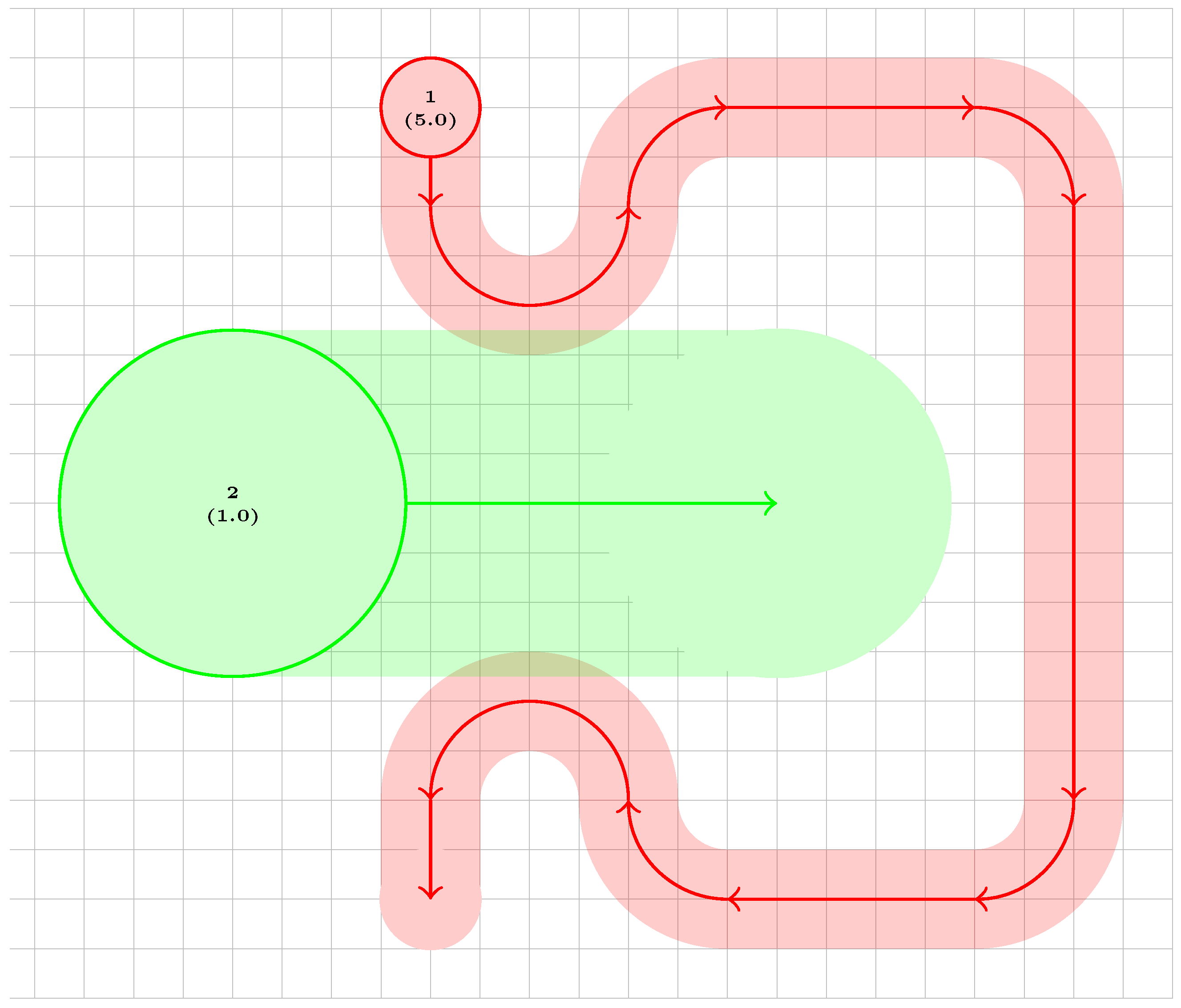
At this point, a careful reader might ask why a different solution representation was not used. Namely, a solution might have multiple resources between the same pair of robots, i.e., robots a and b compete for both $\pi \left(r_1\right)$ and $\pi \left(r_2\right)$. In such a case one could simply assume $\pi \left(r_1\right)=\pi \left(r_2\right)$, significantly reducing the solution space. However, there exist instances for which such “matching” policy is not optimal. For example, consider instance from Figure 3. Here there are only two resources, but robot 2 acquires them at the same time, while robot 1 acquires them separately. For this instance the possible solutions are ${\pi }_1=(0,0)$, ${\pi }_2=(0,1)$, ${\pi }_3=(1,0)$, and ${\pi }_4=(1,1)$. A simple brute force algorithm results in $C_{\max }\left({\pi }_1\right)=16.98$, $C_{\max }\left({\pi }_2\right)=11.00$, and $C_{\max }\left({\pi }_3\right)=C_{\max }\left({\pi }_4\right)=17.96$. Thus, ${\pi }^{*}={\pi }_2$. In general, the idea of such “matching” between some values of $\pi$ is interesting, but determining which elements of $\pi$ can be safely matched is non-trivial.

5. Solving Algorithms

In this section we describe the algorithms used to solve the aforementioned problem. We considered two types of algorithms: constructive algorithms and metaheuristics.

5.1. Constructive Algorithms

Constructive algorithms work by building a single solution according to some policy, often called a dispatch rule, and are popular in many applications, including scheduling [23], particularly in computer networks, high-performance computing, and operating systems [29,32]. The general procedure is similar to solution evaluation shown in Section 4.2, except that algorithm starts with empty $\pi$, which is constructed on-the-fly as the algorithm makes decisions according to its policy. As a result, such algorithms are simple and have short running time, but are usually not optimal, hence they are also heuristics. Below we list all 14 implemented constructive algorithms.

5.1.1. Lower Number First

One of the simplest and fastest algorithms is lower number first, or LNF, done simply by setting $\pi =(0,0,\dots ,0)$. This means that for every resource r that has robots a and $b>a$ competing for it, the policy is for a to acquire r first. Of course, as explained earlier, this rule might be temporarily overlooked if type II deadlock occurs. This algorithm can be seen as deterministic version of random algorithms, since we can simply re-order the robots, in which case LNF might return a different solution.

5.1.2. First-In First-Out

First-in first-out, or FIFO (also known as first-come first-served (FCFS), earliest arrival first (EAF), etc., depending on context), is a very basic and popular algorithm in many optimization, scheduling, and dispatching problems. For this algorithm, the policy is that the first robot to reach the beginning of the sector will be prioritized to enter it first. In practice, we keep a queue, initially empty, for every resource r. When robot a wants to enter a conflicting sector, it adds itself to queues for all required sectors. Next, we compute robot priority as an average of its position in all the relevant queues (similar to what was shown in Section 4) and a will be considered “first in” only when its priority is lowest among all robots queued alongside him in the relevant queues. Of course, a also needs to clear the regular conditions for sector entry. Thus, a will proceed only when (1) required resources are free, (2) resulting state is safe, and (3) a is considered “first in”. In such a case a enters the new sector, removes itself from all relevant queues, and modifies $\pi$ accordingly. After this, similar to solution evaluation, the procedure terminates and $\pi$ will hold the constructed solution.

5.1.3. Shortest Distance First

Shortest distance traveled first (SDTF) is an algorithm that prioritizes robots that have traveled the least distance from their starting positions. In our implementation, when robot a wants to enter a sector, the distance traveled so far by a is computed and then compared against the distance traveled by other robots who are competing over the resources a wants to acquire. It should be noted that when a robot enters a sector, it is removed from the queues of all resources it has just acquired. Thus, robot a is compared only against robots that have yet to reach this point—robots that have already passed this point are not compared against a. We will also consider another variant of SDFT: our objective, the makespan, is based on time rather than distance. Thus, in the second variant the distance traveled is divided by robot speed and the resulting algorithms is called shortest time traveled first (STTF). Note that we count only the time spent moving, as total time spent so far is identical for all robots.

Next, we define two more algorithms that are similar to SDFT and STTF, but that consider remaining distance (time) rather than traveled. The resulting algorithms are shortest distance remaining first (SDRF) and shortest time remaining first (STRF). Finally, we introduce two algorithms that count the total robot path instead of splitting it into traveled-so-far and yet-to-travel part. Those algorithms are called shortest overall distance first (SODF) and shortest overall time first (SOTF).

5.1.4. Longest Distance Variants

Finally, we also define complementary algorithms to the ones defined above, which differ in that they prioritize longest distances instead of shortest. Thus, this leads to definition of the following six additional algorithms:

• Longest distance traveled first (LDTF) and longest time traveled first (LTTF).
• Longest distance remaining first (LDRF) and longest time remaining first (LTRF).
• Longest overall distance first (LODF) and longest overall time first (LOTF).

5.2. Metaheuristics

The constructive algorithms presented in the previous subsection are fast and simple, but they are not enough in all cases. A proof of that is supplied by the counterexample instance presented in Figure 4. For this very simple two-robot instance all 14 constructive algorithms obtained makespan of either 28.26 or 31.26. However, a simple brute force algorithm proved that the optimal makespan in this case is 23.85. This means that the constructive algorithms were 17% and 31% away from the optimum. Thus, alternative solving methods are required. Since exact methods are too time-consuming, we will propose two metaheuristic algorithms, described below. It should also be noted that both proposed metaheuristics could be easily modified into parallel algorithms to vastly decrease computation times while run in many-core or distributed computing environments. For the artificial bee colony, this could be achieved by assigning a number of bees to a given thread or network node. Similarly, for the taboo search, a number of solutions from the neighborhood could be assigned to a single thread/node.

5.2.1. Artificial Bee Colony

Artificial bee colony, or ABC, is a popular population-based probabilistic metaheuristic and was previously used for robot path planning and collision avoidance (see papers [10,11,12,33] for details). Moreover, ABC is both effective and simple to implement, with only a few tuning parameters required.

ABC uses food sources as solutions. Initially a population of p food sources is created and each food source k has its counter $c_k$ set to 0. This results in p different solutions ${\pi }_k$ for $k\in \{1,2,\dots ,p\}$. These solutions are created randomly. Then main algorithm loop starts with each iteration consisting of three phases. In phase 1, a worker bee is sent to each food source and tries to improve it. In our case, for a given solution ${\pi }_k$ we transform it into solution ${\pi }_k^{\prime }$ by flipping a random bit r, i.e., ${\pi }_k^{\prime }\left(r\right)$ is set to ${\pi }_k\left(r\right)$. The resulting solution ${\pi }_k^{\prime }$ is evaluated. If $C_{\max }\left({\pi }_k^{\prime }\right)$ is better than $C_{\max }\left({\pi }_k\right)$, then ${\pi }_k^{\prime }$ replaces ${\pi }_k$ and $c_k$ is set to zero. Otherwise, ${\pi }_k$ stays and $c_k$ increases by 1. In essence, this phase implements the standard valley descent local search procedure with multiple solutions.

Phase 2 is similar to phase 1 with one major difference. In phase 1, the k-th improvement is carried out for the k-th food source. In phase 2, the food source for the k-th improvement is random, but with assumption that better food sources have higher chance of being “tended to”. As a result, statistically, good food sources will be improved multiple times in a single iteration, while bad food sources will receive less attention. In practice, many methods exist for such randomization, in our case we have employed the roulette-wheel selection via stochastic acceptance shown in [34], which guarantees food source choice in time $\mathcal{O}\left(1\right)$.

Finally, in phase 3 each food source k is checked for the value of its counter $c_k$. If $c_k$ is higher than some limit value $\mathit{maxCount}$ then ${\pi }_k$ is deemed non-promising and is replaced with random solution and $c_k$ is set to zero again. With this, phase 3 allows abandoning food sources that fail to improve the solution quality, leading to discovering of new food sources.

Regardless of phase, each time a new solution $\pi$ is generated, its quality is compared to best found solution so far ${\pi }_{\mathrm{best}}$ and if $\pi$ is better, it replaces ${\pi }_{\mathrm{best}}$. The algorithm stops after a fixed number of iterations $\mathit{maxIter}$ is reached with p, $\mathit{maxCount}$, and $\mathit{maxIter}$ as parameters. The overview of ABC method is shown in Algorithm 1.

Algorithm 1: Artificial bee colony (method outline).

5.2.2. Taboo Search

Taboo search (TS) is a local search metaheuristic. It is usually more complex to formulate than ABC, but TS can be made to be fully deterministic algorithm. Moreover, the authors have previously employed this metaheuristic for several discrete optimization problems (check, for example, papers [35,36]), where TS has proved its efficiency.

TS is an iterative algorithm as well. Its outline is shown in Algorithm 2. First, an initial solution ${\pi }_{\mathrm{init}}$ is chosen. In our case it is the FIFO constructive algorithm, but other options are possible as well. Then, in each iteration for a current solution $\pi$ a neighborhood $\mathcal{N}\left(\pi \right)$ is generated, where each neighbor ${\pi }_r$ is created from $\pi$ by flipping the r-th bit in $\pi$ (thus, the neighborhood has R elements). After all neighbors are generated and evaluated, the best of those neighbors ${\pi }_{\mathcal{N}}$ replaces $\pi$, regardless whether ${\pi }_{\mathcal{N}}$ improves $\pi$ or not.

In order to help the algorithm to escape local optima, a taboo list is used. When ${\pi }_{\mathcal{N}}$ is chosen to replace $\pi$ the move that led to this becomes forbidden for number of iterations defined by cadence parameter c. We have used an implementation that allows all taboo list operations in time $\mathcal{O}\left(1\right)$. Additionally, we employ aspiration criterion, that allows to ignore the taboo list if ${\pi }_r$ is better than the best known solution so far.

Algorithm 2: Taboo search (method outline).

As with ABC, each time a new solution is accepted, it is compared against best known solution ${\pi }_{\mathrm{best}}$ and replaces it if it is better. The algorithm finishes when the number of iterations $\mathit{maxIter}$ is reached. Values c, $\mathit{maxIter}$, and ${\pi }_{\mathrm{init}}$ are the parameters of the method.

6. Computer Experiment

In this section, we present the results of a computer experiment on a set of problem instances. We will start by describing the instance generation procedure, including the uncertain data assumptions, as well as the quality of measure used to compare algorithms. Then we will present the results and discuss them.

6.1. Instance Generation

The instance generation procedure is as follows. First, we assume a bounding rectangle from point $(0,0)$ to $(50,50)$. For each of n robots the starting position is chosen randomly outside of the bounding rectangle (we keep a margin of 2 away from the rectangle). The robot radius is drawn from uniform distribution with range $[0.5,2]$ i.e., ${\varphi }_a\sim \mathcal{U}(0.5,2)$. Similarly, for robot speed we have $v_a\sim \mathcal{U}(0.5,2.5)$. The robot path consists of $60-3n$ segments (allowing for shorter paths for more robots). We take care that when an arc follows a line segment, the arc starts angled correctly to the line segment (i.e., no sharp turns for robots). Due to this, if a line segment would follow another line segment, it would have the same angle, thus such line segments can be merged, therefore the path alternates between line segments and arcs. For each line its length is drawn from $\mathcal{U}(2,37)$ (maximum is around 75% of the bounding rectangle width). A safety mechanism is employed: if a path would lead the robot out of the bounding rectangle, the segment is rejected and a new one is attempted. After 20 unsuccessful attempts, a 180 degrees turn-around arc is used instead.

The above considers only the deterministic case. For the uncertain case, we proceed as follows. For a given instance I we obtain a modified instance $I\left(Y\right)$ by replacing all sector lengths $l_i$ with values $l_i{y}_i$, where $y_i$ is a realization of random variable Y. In other words, $y_i$ is a scaling parameter of the original sector lengths. Index i is used to denote that $y_i$ and $y_j$ are different realizations of Y. Additionally, since we assume robot speed is constant, changes to travel distances translate directly to changes to travel time, modeling uncertainty in robot movement. As for random variable Y, we would like to have the expected value of $l_{i}Y$ be equal to $l_i$ (i.e., the expected sector length is equal to its nominal value), so the expected value of Y should be 1. We also assume standard deviation parameter ${\sigma }_Y$. Thus:

$$\mathbb{E}\left[Y\right]={\mu }_Y=1,$$

(12)

$$\mathbb{V}\left[Y\right]={\sigma }_Y^2,$$

(13)

where $\mathbb{E}$ and $\mathbb{V}$ are expectation and variance operators, respectively.

Since sector lengths have to be positive, we choose to model Y using log-normal distribution, i.e., $Y\sim LogNormal(\mu ,{\sigma }^2)$. In order for Y to have expected value and standard deviation assumed in (12) and (13), we set $\mu$ and $\sigma$ to:

$$\mu =ln\left(\frac{{\mu }_Y^2}{\sqrt{{\mu }_Y^2+{\sigma }_Y^2}}\right)=ln\left(\frac{1}{\sqrt{1+{\sigma }_Y^2}}\right),$$

(14)

$${\sigma }^2=ln\left(1+\frac{{\sigma }_Y^2}{{\mu }_Y^2}\right)=ln\left(1+{\sigma }_Y^2\right).$$

(15)

Using the above instance generator, we have prepared a benchmark of 50 instances, 10 for each size $n\in \{2,3,4,5,6\}$. Instances are numbered with subsequent natural numbers i.e., instances for $n=2$ are numbered 1 through 10, for $n=3$ are numbered 11 through 20 and so on. Number of sectors ranges from 38 to 693, while number of resources ranges from 21 to 4007. An example of generated instance for four robots is visualized in Figure 5. Let us note that the number of resources identified for this, relatively small, instance with only four robots was equal to 419, yielding a solution space with $2^{419}$ solutions. This is roughly equivalent to the solution space of traveling salesman problem with approximately 84 cities.

6.2. Measure of Quality

Concerning the measure of quality, we will use percentage relative deviation, or PRD, defined as follows. Let $\mathcal{M}=\{\mathit{LNF},\mathit{FIFO},\dots ,\mathit{ABC},\mathit{TS}\}$ be the set of solving methods (algorithms) we want to compare, described in Section 5. Let ${\pi }_m^I$ be solution obtained by method $m\in \mathcal{M}$ for problem instance I. Then for solving method m and instance I the value ${\mathit{PRD}}_m^I$ is equal to:

$${\mathit{PRD}}_m^I=\frac{C_{\max }\left({\pi }_m^I\right)}{{min}_{z\in \mathcal{M}}{C}_{\max }\left({\pi }_z^I\right)}.$$

(16)

In other words, we compare given method m against a reference method $z\in \mathcal{M}$, which is the one which obtained the best (lowest) makespan for that instance I. Thus, $C_{\max }\left({\pi }_z^I\right)$ serves as the best-known solution for instance I and z may change between different instances. For example, if $C_{\max }\left({\pi }_z^I\right)=250$ and $C_{\max }\left({\pi }_m^I\right)=350$ then ${\mathit{PRD}}_m^I=1.4$, meaning that method m obtained 40% worse result than best-known method z. Thus, $\mathit{PRD}$ allows us to normalize the results, removing the bias caused by different instances and different problem sizes resulting in different ranges of observed makespans.

For the case with uncertain data we proceed slightly different. For a given instance I we create a sample of 100 uncertain instances denoted $I{\left(Y\right)}_1$ through $I{\left(Y\right)}_{100}$. All instances draw from the same distribution, but each will be slightly different. Next, for solving method m, m is used to solve the original (deterministic) instance I with nominal values, obtaining solution ${\pi }_m^I$. Finally, we compute the value of $C_{\max }\left({\pi }_m^{I\left(Y\right)}\right)$ as the arithmetic mean:

$$C_{\max }\left({\pi }_m^{I\left(Y\right)}\right)=\frac{1}{100}\sum _{i=1}^{100}{C}_{\max }\left({\pi }_m^{I{\left(Y\right)}_i}\right),$$

(17)

thus, $C_{\max }\left({\pi }_m^{I\left(Y\right)}\right)$ estimates the expected value of makespan obtained by method m. Values $C_{\max }\left({\pi }_m^{I\left(Y\right)}\right)$ and $C_{\max }\left({\pi }_z^{I\left(Y\right)}\right)$ are then used to define ${\mathit{PRD}}_m^{I\left(Y\right)}$, similarly to (16).

6.3. Implementation and Equipment Details

All algorithms were implemented in Julia programming language (version 1.7.2) and run on a server with the AMD Ryzen Threadripper 3990X CPU (2.9 MHz, 64-cores) and 64 GB of RAM under Linux operating systems. Regarding the parameters of the ABC and TS methods, we performed a calibration using a portion of the instance described in Section 6.1, namely 30 instances with $n\in \{2,3,4\}$. For the TS method, four parameters were considered: (1) number of iterations, (2) initial solution, (3) cadence type, and (4) cadence size. For the number of iterations we have considered $\mathit{maxIter}\in \{60,80,100,120\}$. For initial solution we considered ${\pi }_{\mathrm{init}}\in \{\mathrm{FIFO},\mathrm{LDRF},\mathrm{STTF},\mathrm{LNF}\}$. Three cadence types were considered. First, constant cadence with four values $c\in \{10,100,1000,1000\}$. Second, linear cadence $c=\beta \times \mathit{maxIter}$ with four values $\beta \in \{0.2,0.4,0.6,0.8\}$. Lastly, square root variant $c=\gamma \times \sqrt{\mathit{maxIter}}$ with four values $\gamma \in \{0.5,1.0,2.0,4.0\}$. The preliminary research indicated that the best variant was $\mathit{maxIter}=120$, ${\pi }_{m}athrminit=\mathrm{LDRF}$, $c=\beta \times \mathit{maxIter}$, and $\beta =0.4$. It should be noted that out of the four parameters only $\mathit{maxIter}$ has significant (and straightforward) effect on the running time. We have also consciously refrained from using higher number of iterations due to the size of the neighborhood.

Similar, preliminary research was done for the ABC method. Here, we have also assumed an upper bound for the computation time determined by the iteration limit and population size $\mathit{maxIter}\times p$. We have considered values $\mathit{maxIter}\in \{60,80,100,120\}$ and $p\in \{5,10,15,20\}$. Concerning the parameter $\mathit{maxCount}$, we have tested the same values as cadence c for the TS method. The research indicated that the best results were obtained for $\mathit{maxIter}=120$, $p=20$ and linear $\mathit{maxCount}$ with $\beta =0.4$.

6.4. Results

In our experiment we have assumed six different uncertainty scenarios. The first scenario is for deterministic data, i.e., $\sigma =0$. The remaining five scenarios are for progressively increasing robot travel times uncertainty with $\sigma \in \{0.01,0.05,0.1,0.15,0.2\}$. Cases $\sigma =0.01$, $\sigma =0.1$, and $\sigma =0.2$ can be taken to represents slightly, moderately, and largely uncertain data, respectively. First, we show exemplary results for two instances in

Table 2. PRD results for instance no. 13 ($n=3$) with 121 sectors and 132 resources (best three results for each scenario type in bold).

Algorithm	$\mathit{\sigma }=0$	$\mathit{\sigma }=0.01$	$\mathit{\sigma }=0.05$	$\mathit{\sigma }=0.1$	$\mathit{\sigma }=0.15$	$\mathit{\sigma }=0.2$
TS	1.018	1.000	1.000	1.021	1.068	1.041
ABC	1.000	1.026	1.029	1.018	1.063	1.141
LNF	1.604	1.581	1.463	1.414	1.396	1.415
FIFO	1.444	1.097	1.043	1.035	1.032	1.032
SDTF	1.287	1.076	1.037	1.023	1.021	1.025
STTF	1.310	1.073	1.017	1.000	1.000	1.000
LDTF	1.630	1.229	1.167	1.158	1.162	1.183
LTTF	1.630	1.229	1.167	1.158	1.162	1.183
SDRF	1.630	1.229	1.167	1.158	1.162	1.183
STRF	1.630	1.229	1.167	1.158	1.162	1.183
LDRF	1.047	1.301	1.209	1.198	1.192	1.196
LTRF	1.174	1.102	1.186	1.201	1.162	1.193
SODF	1.900	1.384	1.313	1.286	1.284	1.279
SOTF	1.630	1.229	1.167	1.158	1.162	1.183
LODF	1.842	1.581	1.463	1.414	1.396	1.415
LOTF	1.760	1.554	1.395	1.320	1.244	1.274

and

Table 3. PRD results for instance no. 48 ($n=6$) with 546 sectors and 2415 resources (best three results for each scenario type in bold).

Algorithm	$\mathit{\sigma }=0$	$\mathit{\sigma }=0.01$	$\mathit{\sigma }=0.05$	$\mathit{\sigma }=0.1$	$\mathit{\sigma }=0.15$	$\mathit{\sigma }=0.2$
TS	1.000	1.000	1.000	1.000	1.000	1.000
ABC	1.619	1.542	1.614	1.455	1.447	1.499
LNF	2.053	1.897	1.836	1.726	1.699	1.649
FIFO	1.679	1.355	1.314	1.245	1.234	1.197
SDTF	1.900	1.602	1.542	1.457	1.442	1.402
STTF	1.889	1.640	1.590	1.508	1.494	1.454
LDTF	1.615	1.963	1.903	1.799	1.777	1.713
LTTF	2.196	1.821	1.764	1.679	1.670	1.633
SDRF	1.327	1.988	1.927	1.826	1.807	1.756
STRF	1.864	1.987	1.926	1.825	1.804	1.752
LDRF	1.840	1.248	1.209	1.146	1.130	1.101
LTRF	1.258	1.495	1.449	1.370	1.358	1.321
SODF	1.528	1.993	1.932	1.831	1.811	1.760
SOTF	1.864	1.987	1.926	1.825	1.804	1.752
LODF	1.664	1.791	1.737	1.645	1.627	1.580
LOTF	1.677	1.918	1.860	1.761	1.744	1.693

.

For instance, from Table 2 (which already has 132 resources), we observe that the TS and ABC methods provide the best results when the uncertainty is small ($\sigma <0.05$), while the FIFO, SDTF, and STTF algorithms start to outperform them when uncertainty becomes more significant ($\delta \ge 0.05$). However, we still observe that TS and ABC outperform all other tested algorithms, often very significantly (50% to 90% differences). We also note that as $\delta$ increases, the quality of the performance of TS and ABC generally drops, while that of constructive algorithms increases. This is an expected result as constructive rule-based algorithms are usually viewed as more robust. Next, we will discuss the results for instance from Table 3 (which has nearly 20 times more resources). Here, the TS method managed to outperform all other algorithms for all $\delta$ values. On the other hand, ABC is consistently outperformed by three algorithms, but still remains ahead of the remaining ones. Interestingly, this time around the performance of ABC increases with the increase of $\delta$. From the constructive algorithms, FIFO and LDRF obtained the best results. We also note that the general performance gap between algorithms increased compared to instance from Table 2. This is easily seen by comparing the values of LOTF in both tables.

We will now move onto aggregated (average) results grouped by number of robots n, which are shown in

Table 4. Aggregated average PRD results for selected algorithms, grouped by number of robots (best result for each scenario type in bold).

n	Algorithm	$\mathit{\sigma }=0$	$\mathit{\sigma }=0.01$	$\mathit{\sigma }=0.05$	$\mathit{\sigma }=0.1$	$\mathit{\sigma }=0.15$	$\mathit{\sigma }=0.2$
	TS	1.000	1.094	1.094	1.090	1.087	1.083
	ABC	1.000	1.000	1.009	1.017	1.023	1.014
2	FIFO	1.020	1.020	1.021	1.020	1.020	1.017
	SDTF	1.018	1.021	1.019	1.016	1.015	1.011
	LTRF	1.033	1.021	1.021	1.020	1.020	1.017
	TS	1.015	1.013	1.053	1.089	1.103	1.104
	ABC	1.075	1.086	1.112	1.093	1.190	1.141
3	LNF	1.504	1.496	1.475	1.466	1.434	1.420
	FIFO	1.184	1.094	1.074	1.070	1.050	1.045
	LDRF	1.239	1.197	1.183	1.157	1.127	1.113
	LTRF	1.237	1.230	1.227	1.202	1.175	1.159
	TS	1.000	1.022	1.069	1.110	1.146	1.156
	ABC	1.260	1.320	1.300	1.325	1.324	1.384
4	FIFO	1.552	1.334	1.279	1.236	1.218	1.200
	STTF	1.682	1.286	1.242	1.204	1.187	1.179
	LTRF	1.361	1.457	1.401	1.352	1.335	1.317
	TS	1.025	1.136	1.204	1.258	1.301	1.311
	ABC	1.540	1.586	1.638	1.657	1.698	1.578
5	FIFO	1.386	1.358	1.338	1.313	1.312	1.298
	LDRF	1.643	1.529	1.503	1.463	1.444	1.417
	LTRF	1.498	1.676	1.648	1.614	1.601	1.584
	TS	1.000	1.014	1.031	1.038	1.048	1.070
	ABC	1.640	1.635	1.625	1.590	1.578	1.584
6	FIFO	1.437	1.297	1.253	1.214	1.192	1.182
	STTF	1.735	1.314	1.282	1.255	1.250	1.247
	LTRF	1.546	1.349	1.308	1.270	1.258	1.249

. For the sake of brevity, we have restricted ourselves to showing metaheuristics and three best constructive algorithms for each n. In general, we observe that effectiveness of both TS and ABC decreases with increase in $\sigma$. For the best constructive algorithms the relations is opposite—those algorithms improve under uncertainty. TS is also the best algorithm overall, being outperformed only a few times when n is small and $\delta$ is high. ABC is significantly worse, being outperformed by TS and FIFO except for small n and $\delta$. We also observe that FIFO remains fairly effective in almost all cases. SDTF, STTF, LDRF, and LTRF are consequently the next in the effectiveness order. However, all of those constructive algorithms are still often 20% to 70% worse than TS metaheuristic and this effect increases as n increases.

Finally, the aggregated results for all benchmark instances are shown in

Table 5. Aggregated average PRD results for all benchmark instances (three best results for each scenario type in bold).

Algorithm	$\mathit{\sigma }=0$	$\mathit{\sigma }=0.01$	$\mathit{\sigma }=0.05$	$\mathit{\sigma }=0.1$	$\mathit{\sigma }=0.15$	$\mathit{\sigma }=0.2$
TS	1.008	1.056	1.090	1.117	1.137	1.145
ABC	1.303	1.325	1.337	1.337	1.363	1.340
LNF	1.586	1.620	1.590	1.563	1.545	1.531
FIFO	1.316	1.221	1.193	1.170	1.158	1.148
SDTF	1.502	1.316	1.292	1.268	1.254	1.242
STTF	1.509	1.261	1.236	1.213	1.201	1.194
LDTF	1.732	1.617	1.585	1.556	1.540	1.524
LTTF	1.749	1.596	1.564	1.537	1.521	1.505
SDRF	1.723	1.593	1.567	1.537	1.522	1.505
STRF	1.737	1.621	1.593	1.564	1.551	1.536
LDRF	1.437	1.277	1.254	1.227	1.213	1.200
LTRF	1.335	1.347	1.321	1.292	1.278	1.265
SODF	1.734	1.622	1.593	1.562	1.546	1.528
SOTF	1.746	1.628	1.602	1.575	1.561	1.546
LODF	1.761	1.623	1.593	1.562	1.545	1.530
LOTF	1.706	1.615	1.584	1.552	1.536	1.517

. Once again, TS’s average performance is superior to all other tested algorithms. ABC remains competitive for deterministic case, but is outclassed by several algorithms (most notably FIFO) for uncertain cases. We also note that the implemented metaheuristics are fairly robust: TS and ABC suffered only 13.6% and 2.8% drop in PRD between the $\sigma =0$ and $\sigma =0.2$ cases, respectively. As previously, unlike the metaheuristics, the constructive algorithms become more competitive as uncertainty in the data increases. This is most visible for STTF, which gains 26.4% in PRD between the $\sigma =0$ and $\sigma =0.2$ cases, although it is still slightly behind FIFO. On the other hand, LNF improves the least by only 3.6%. Out of all the constructive algorithms, FIFO, STTF, and LDRF obtained the best results for all $\sigma$ scenarios. As for the worst algorithms, LODF, SOTF, and LTTF performed the worst for the $\sigma =0$ case, while SOTF, STRF, LODF, SODF, and LNF performed the worst for $\sigma =0.2$.

6.5. Discussion

While the presented research confirmed that the metaheuristic methods are effective with regards to makespan optimization for the considered MMRS, they suffer from vastly longer execution time compared to simple constructive algorithms. This is especially true for the TS metaheuristic, which is more effective but slower than ABC. Sometimes the running time is not an issue, but in some contexts (e.g., robot paths are unknown in advance) such a drawback might not be acceptable. Thus, here we discuss a few options to reduce this running times of both TS and ABC methods:

• The solution evaluation procedure is by far the most time-consuming part of both methods. Thus, any reduction in its running time would benefit the overall algorithm. One possibility would be to abandon the “state safety” check. This would allow for a type I deadlock, but such solution would simply be treated as infeasible and rejected. It remains an open question how such change would affect the quality of both methods.
• As mentioned in Section 4, it might be possible to reduce the solution size by forcing some of its element to always be equal to each other. This can be done optimally (“match” only elements that are sure to be matched in the optimal solution) or approximately (guess which elements could be matched, risking reduced solution quality).
• Parallel computing: running time can be significantly reduced by dividing work among many processors. Both methods can be parallelized fairly well as neighbors in TS can be handled independent from each other. This is made easier by solution evaluation function being complex (this is unlike problems with $\mathcal{O}\left(1\right)$ neighbor evaluation which are harder to parallelize). This is similar for food sources in ABC.
• Lastly, we can reduce running time significantly by decreasing the population size for ABC or by checking only a small (e.g., 10%) number of neighbors in TS. Moreover, we can simply reduce the iteration limit for either method. Both actions will generally affect the quality of obtained solutions, though it might be possible to reduce time significantly while still obtaining comparable results.

Nonetheless, a situation might occur in which metaheuristics will not be applicable due to time restriction or will not be able to provide satisfactory results in that time. In such cases, one needs to rely on constructive algorithms instead. For this, the best option appears to be the FIFO algorithm—for $\sigma =0.2$ it is only 0.3% worse than TS. For the deterministic case, FIFO is considerably (30.1%) worse than TS, but still outclasses other algorithms. STTF and LDRF were also fairly effective, though to a lesser extent. The remaining constructive algorithms consistently proved to be considerably worse. Surprisingly, the STTF, LTTF, STRF, LTRF, STF, and LOTF algorithms not only were not much better than their distance-based counterparts, but half the time they proved to be actually worse. This could be a coincidence, but it seems unlikely, as 50 random instances were used and robot speeds ranged considerably between each other.

7. Conclusions

In the paper we have considered the process of navigation for multiple mobile robots system with fixed paths operating in a real-valued two-dimensional space. Unlike existing works, we have tackled two problems at once: (1) optimization of robot moving schedules to minimize the makespan and (2) collision and deadlock avoidance. Based on the concept of sectors, we proposed a reformulation of the initial problem. This made it possible to disregard the specific shapes of robot paths, simplifying the problem.

We then introduced a binary solution representation based on resources derived from sectors. This allowed us to turn the original continuous optimization problem into discrete optimization formulation with vastly reduced solution space. However, we have shown that the resulting solution space is still large, even for relatively simple problem instances with only two or three robots. We have identified two types of deadlocks: (1) a classic deadlock caused by resources availability and (2) a deadlock caused by the solution-enforced robot queuing order. We have proposed approaches to avoid type I deadlocks while also resolving type II deadlocks.

For solving method, we have implemented two metaheuristic algorithms: taboo search (TS) and artificial bee colony (ABC). We have also implemented 14 constructive algorithms based on simple dispatch rules. Next, we provided 50 random problem instances as a testing benchmark, with number of resources ranging from dozens to several thousands. The results proved that TS outperforms other algorithms for both deterministic and uncertain cases. A few constructive algorithms (including FIFO, STTF, and LDRF) also obtained good results, lessening their gap to TS as uncertainty grows. ABC provided the best results for small instances, but its performance quickly dropped below that of TS, FIFO, STTF, and LDRF. Nonetheless, ABC managed to outperform the remaining constructive algorithms.

References

1. Roszkowska, E.; Jakubiak, J. Control synthesis for multiple mobile robot systems. Trans. Inst. Meas. Control 2021. [Google Scholar] [CrossRef]
2. Roszkowska, E. Provably Correct Closed-Loop Control for Multiple Mobile Robot Systems. In Proceedings of the 2005 IEEE International Conference on Robotics and Automation, Barcelona, Spain, 18–22 April 2005; pp. 2810–2815. [Google Scholar] [CrossRef]
3. Reveliotis, S.; Roszkowska, E. Conflict Resolution in Free-Ranging Multivehicle Systems: A Resource Allocation Paradigm. IEEE Trans. Robot. 2011, 27, 283–296. [Google Scholar] [CrossRef] [Green Version]
4. Roszkowska, E.; Reveliotis, S. A Distributed Protocol for Motion Coordination in Free-Range Vehicular Systems. Automatica 2013, 49, 1639–1653. [Google Scholar] [CrossRef] [Green Version]
5. Kloetzer, M.; Mahulea, C.; Colom, J.M. Petri net approach for deadlock prevention in robot planning. In Proceedings of the 2013 IEEE 18th Conference on Emerging Technologies &Factory Automation (ETFA), Cagliari, Italy, 10–13 September 2013; pp. 1–4. [Google Scholar] [CrossRef]
6. Gakuhari, H.; Jia, S.; Takase, K.; Hada, Y. Real-Time Deadlock-Free Navigation for Multiple Mobile Robots. In Proceedings of the 2007 International Conference on Mechatronics and Automation, Harbin, China, 5–8 August 2007; pp. 2773–2778. [Google Scholar] [CrossRef]
7. Čáp, M.; Novák, P.; Kleiner, A.; Selecký, M. Prioritized Planning Algorithms for Trajectory Coordination of Multiple Mobile Robots. IEEE Trans. Autom. Sci. Eng. 2015, 12, 835–849. [Google Scholar] [CrossRef] [Green Version]
8. Ferrera, E.; Castaño, A.R.; Capitán, J.; Ollero, A.; Marrón, P.J. Decentralized collision avoidance for large teams of robots. In Proceedings of the 2013 16th International Conference on Advanced Robotics (ICAR), Montevideo, Uruguay, 25–29 November 2013; pp. 1–6. [Google Scholar] [CrossRef]
9. Ferrera, E.; Capitán, J.; Castaño, A.R.; Marrón, P.J. Decentralized safe conflict resolution for multiple robots in dense scenarios. Robot. Auton. Syst. 2017, 91, 179–193. [Google Scholar] [CrossRef]
10. Bhattacharjee, P.; Rakshit, P.; Goswami, I.; Konar, A.; Nagar, A.K. Multi-robot path-planning using artificial bee colony optimization algorithm. In Proceedings of the 2011 Third World Congress on Nature and Biologically Inspired Computing, Salamanca, Spain, 19–21 October 2011; pp. 219–224. [Google Scholar] [CrossRef]
11. Liang, J.H.; Lee, C.H. Efficient collision-free path-planning of multiple mobile robots system using efficient artificial bee colony algorithm. Adv. Eng. Softw. 2015, 79, 47–56. [Google Scholar] [CrossRef]
12. Mansury, E.; Nikookar, A.; Salehi, M.E. Artificial Bee Colony optimization of ferguson splines for soccer robot path planning. In Proceedings of the 2013 First RSI/ISM International Conference on Robotics and Mechatronics (ICRoM), Tehran, Iran, 13–15 February 2013; pp. 85–89. [Google Scholar] [CrossRef]
13. Kumar, S.; Muni, M.K.; Pandey, K.K.; Chhotray, A.; Parhi, D.R. Path planning and control of mobile robots using modified Tabu search algorithm in complex environment. In Proceedings of the International Conference on Artificial Intelligence in Manufacturing & Renewable Energy (ICAIMRE), Bhubaneswar, India, 25–26 October 2019. [Google Scholar]
14. Balan, K.; Luo, C. Optimal Trajectory Planning for Multiple Waypoint Path Planning using Tabu Search. In Proceedings of the 2018 9th IEEE Annual Ubiquitous Computing, Electronics & Mobile Communication Conference (UEMCON), New York, NY, USA, 8–10 November 2018; pp. 497–501. [Google Scholar] [CrossRef]
15. Lygeros, J.; Godbole, D.; Sastry, S. Verified hybrid controllers for automated vehicles. IEEE Trans. Autom. Control 1998, 43, 522–539. [Google Scholar] [CrossRef] [Green Version]
16. Tomlin, C.; Pappas, G.; Sastry, S. Conflict resolution for air traffic management: A study in multiagent hybrid systems. IEEE Trans. Autom. Control 1998, 43, 509–521. [Google Scholar] [CrossRef] [Green Version]
17. Pecora, F.; Cirillo, M.; Dimitrov, D. On mission-dependent coordination of multiple vehicles under spatial and temporal constraints. In Proceedings of the 2012 IEEE/RSJ International Conference on Intelligent Robots and Systems, Vilamoura, Algarve, Portugal, 7–12 October 2012; pp. 5262–5269. [Google Scholar] [CrossRef]
18. Andreasson, H.; Bouguerra, A.; Cirillo, M.; Dimitrov, D.N.; Driankov, D.; Karlsson, L.; Lilienthal, A.J.; Pecora, F.; Saarinen, J.P.; Sherikov, A.; et al. Autonomous Transport Vehicles: Where We Are and What Is Missing. IEEE Robot. Autom. Mag. 2015, 22, 64–75. [Google Scholar] [CrossRef]
19. Grover, J.S.; Liu, C.; Sycara, K. Deadlock analysis and resolution for multi-robot systems. In Proceedings of the International Workshop on the Algorithmic Foundations of Robotics, Oulu, Finland, 21–23 June 2021; pp. 294–312. [Google Scholar]
20. Akella, S.; Hutchinson, S. Coordinating the motions of multiple robots with specified trajectories. In Proceedings of the 2002 IEEE International Conference on Robotics and Automation (Cat. No. 02CH37292), Washington, DC, USA, 11–15 May 2002; Volume 1, pp. 624–631. [Google Scholar] [CrossRef]
21. Wang, Z.; Gombolay, M. Learning Scheduling Policies for Multi-Robot Coordination With Graph Attention Networks. IEEE Robot. Autom. Lett. 2020, 5, 4509–4516. [Google Scholar] [CrossRef]
22. Lin, S.; Liu, A.; Wang, J.; Kong, X. A Review of Path-Planning Approaches for Multiple Mobile Robots. Machines 2022, 10, 773. [Google Scholar] [CrossRef]
23. De Frene, E.; Schatteman, D.; Herroelen, W.; Van de Vonder, S. A Heuristic Methodology for Solving Spatial Resource-Constrained Project Scheduling Problems. 2007. Available online: https://ssrn.com/abstract=1089355 (accessed on 30 September 2022).
24. Prashant Reddy, J.; Kumanan, S.; Krishnaiah Chetty, O. Application of Petri nets and a genetic algorithm to multi-mode multi-resource constrained project scheduling. Int. J. Adv. Manuf. Technol. 2001, 17, 305–314. [Google Scholar] [CrossRef]
25. Lawley, M.; Reveliotis, S.; Ferreira, P. A correct and scalable deadlock avoidance policy for flexible manufacturing systems. IEEE Trans. Robot. Autom. 1998, 14, 796–809. [Google Scholar] [CrossRef] [Green Version]
26. Golmakani, H.; Mills, J.; Benhabib, B. Deadlock-free scheduling and control of flexible manufacturing cells using automata theory. IEEE Trans. Syst. Man, Cybern. Part A Syst. Humans 2006, 36, 327–337. [Google Scholar] [CrossRef]
27. Sun, Y.; Chung, S.H.; Wen, X.; Ma, H.L. Novel robotic job-shop scheduling models with deadlock and robot movement considerations. Transp. Res. Part E Logist. Transp. Rev. 2021, 149, 102273. [Google Scholar] [CrossRef]
28. Dang, Q.V.; Nguyen, C.T.; Rudová, H. Scheduling of mobile robots for transportation and manufacturing tasks. J. Heuristics 2019, 25, 175–213. [Google Scholar] [CrossRef]
29. Sun, H.; Elghazi, R.; Gainaru, A.; Aupy, G.; Raghavan, P. Scheduling Parallel Tasks under Multiple Resources: List Scheduling vs. In Pack Scheduling. In Proceedings of the 2018 IEEE International Parallel and Distributed Processing Symposium (IPDPS), Vancouver, BC, Canada, 21–25 May 2018; pp. 194–203. [Google Scholar] [CrossRef] [Green Version]
30. Gopalan, K.; Kang, K.D. Coordinated allocation and scheduling of multiple resources in real-time operating systems. In Proceedings of the Workshop on Operating Systems Platforms for Embedded Real-Time Applications, Pisa, Italy, 4–6 July 2007; p. 48. [Google Scholar]
31. Reveliotis, S.; Roszkowska, E. On the Complexity of Maximally Permissive Deadlock Avoidance in Multi-Vehicle Traffic Systems. IEEE Trans. Autom. Control 2010, 55, 1646–1651. [Google Scholar] [CrossRef]
32. Rudy, J.; Zelazny, D. Memetic algorithm approach for multi-criteria network scheduling. In Proceedings of the International Conference On ICT Management for Global Competitiveness And Economic Growth In Emerging Economies, Wroclaw, Poland, 17–18 September 2012; pp. 247–261. [Google Scholar]
33. Wang, Z.; Li, M.; Dou, L.; Li, Y.; Zhao, Q.; Li, J. A novel multi-objective artificial bee colony algorithm for multi-robot path planning. In Proceedings of the 2015 IEEE International Conference on Information and Automation, Lijiang, China, 8–10 August 2015; pp. 481–486. [Google Scholar] [CrossRef]
34. Lipowski, A.; Lipowska, D. Roulette-wheel selection via stochastic acceptance. Phys. A Stat. Mech. Its Appl. 2012, 391, 2193–2196. [Google Scholar] [CrossRef] [Green Version]
35. Rudy, J.; Pempera, J.; Smutnicki, C. Improving the TSAB algorithm through parallel computing. Arch. Control. Sci. 2020, 30, 411–435. [Google Scholar]
36. Idzikowski, R.; Rudy, J.; Gnatowski, A. Solving Non-Permutation Flow Shop Scheduling Problem with Time Couplings. Appl. Sci. 2021, 11, 4425. [Google Scholar] [CrossRef]
Figure 1. Example base problem instances with 3 robots. Each robot is portrayed with a different color. Circles denote robot starting positions. Circle labels show robot number and speed (in parentheses).
Processes 10 02087 g001
Figure 2. Exemplary instance for 3 robots. The white dot and circle denote a position and disk range somewhere along the path of robot 3. The dashed lines represent the borders of sectors (which will be explained further on).
Processes 10 02087 g002
Figure 3. Counterexample instance for solution representation.
Processes 10 02087 g003
Figure 4. Counterexample instance for constructive algorithms.
Processes 10 02087 g004
Figure 5. Visualization of benchmark instance 21 ( n = 4 ) with 236 sectors and 419 resources.
Processes 10 02087 g005