
Experimental Research on Oil–Water Flow Imaging in Near-Horizontal Well Using Single-Probe Multi-Position Measurement Fluid Imager


1
College of Geophysics and Petroleum Resources, Yangtze University, Wuhan 430100, China
2
Key Laboratory of Exploration Technologies for Oil and Gas Resources (Yangtze University), Ministry of Education, Wuhan 430100, China
*
Author to whom correspondence should be addressed.
Processes 2022, 10(6), 1051; https://doi.org/10.3390/pr10061051
Submission received: 27 February 2022
/
Revised: 17 May 2022
/
Accepted: 18 May 2022
/
Published: 25 May 2022
(This article belongs to the Special Issue New Challenges in Advanced Process Control in Petroleum Engineering)
Abstract
:To obtain local flow velocity and holdup for oil–water in a near-horizontal well, array probes were adopted in the cross section of the wellbore. In this study, a fluid flow imaging logging tool called the single-probe multi-position measurement fluid imager (SPFI) was developed, which consisted of only a single turbine flowmeter and a single capacitance holdup probe. Most importantly, it could collect local velocity and holdup information at different locations along the vertical direction of the wellbore diameter. Firstly, in the large-diameter multi-phase flow simulation test loop, the instrument was placed at five different positions along the wellbore cross section to perform simulated measurements in different wellbore deviation angles and oil–water flowrates. Secondly, the experiment data was analyzed, and the experiment flow pattern chart, instrument response coefficient, and rule of the instrument response were obtained. At the same time, the calculation methods of local holdup and local velocity were derived. Thirdly, by combining the interpolation algorithm, velocity imaging and holdup imaging were implemented, and the stratified flow model was used to calculate the flowrate of each phase. Finally, this study provides technology support for production profile data interpretation using the fluid flow imaging tool for oil–water in a near-horizontal well.
1. Introduction
In order to distinguish the complex flow pattern structure of multi-phase flow in deviated and horizontal wells, such as the stratified flow and dispersed flow, it is necessary to conduct interventional sampling measurements of the fluid in the cross section of the wellbore at different locations as much as possible [1,2,3]. The flow pattern is significant since by observing the flow pattern in the wellbore, we can understand the oil and water distribution state in the wellbore and guide the accuracy of the data measured by the instrument. By counting the flow patterns under different experimental conditions, the distribution of oil and water in the well can be predicted in the future. Multi-phase flow has been studied for many years [4,5,6,7,8,9,10,11], and the current commercial multi-phase flow measurement instruments for horizontal wells mainly use an array of probes consisting of capacitance probes, resistance probes, and turbines to cover the whole wellbore cross section for measurement, such as the Schlumberger FloScan Imager (FSI, six Floview probes, six GHOST probes, five microturbine flowmeters) [12,13], Multiple Array Production Suite (MAPS) from Sondex UK (Capacitance Array tool (CAT) with 12 capacitance probes, Resistance Array tool (RAT) with 12 resistance probes, and Spinner Array tool (SAT) with six microturbine flowmeters) [14,15,16,17], Array Fluid Resistivity Meter (AFR, 12 resistance probes), and Array Fluid Velocity Meter (AFV, six turbine flowmeters) from Hunter Canada [18] and other instruments. The above-mentioned array probe combination instruments can simultaneously measure fluid information at different positions in the wellbore.
The novelty of this study is that different from other array instruments, a single-probe multi-position measurement fluid imager (SPFI) was used, which included only a single turbine flowmeter and a single capacitance holdup probe. The SPFI has a smaller volume in the wellbore and has less effect on fluid flow. Since it can measure the local flow velocity and holdup information at different positions along the vertical direction of the wellbore diameter, it can also perform real-time monitoring of fluid flow imaging [19,20]. In order to evaluate the test effect of the SPFI instrument, we used it to conduct the oil–water simulation measurement experiment in near-horizontal wells at five different heights in the multi-phase flow loop. After data processing, the flow pattern diagram and tool response law under different wellbore deviation angles and different oil–water flowrates were obtained, and velocity imaging and water holdup imaging under different conditions were also achieved. Finally, the flowrate of each phase of the stratified flow was calculated and verified. The research results in this study are helpful to realize the accurate interpretation of the logging data of the oil–water flow profile of the near-horizontal well.
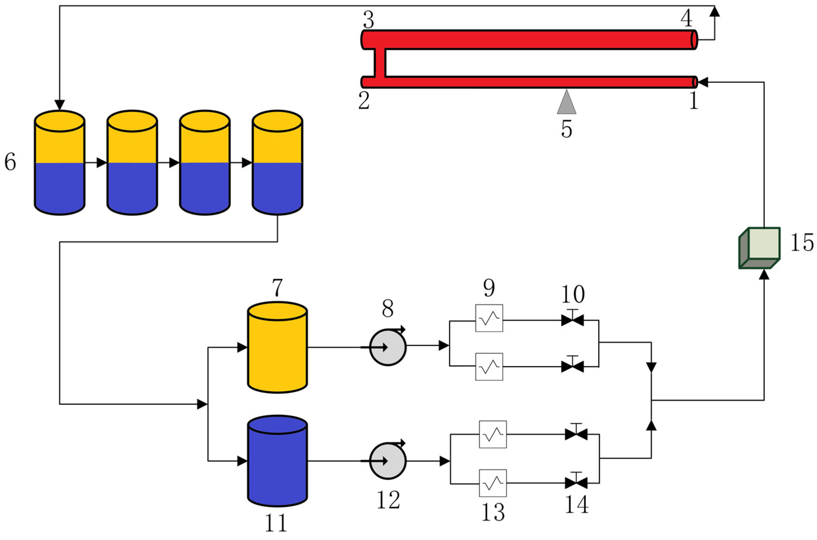
2. Overview of Flow Experiments
As shown in Figure 1, this experiment was performed on the multi-phase flow simulation device for horizontal and high-angle deviated well of Yangtze University. The simulated wellbore was 12 m long and had an inner diameter of 124 mm, and the medium was tap water and white oil. Under room temperature and normal pressure, combined with the actual production situation of the oil field, we set the total flowrate of oil and water to 50, 70, 100, 120, 160, 200, 250, and 300 . The water cut was 0%, 10%, 20%, 40%, 50%, 60%, 70%, 80%, 90%, and 100%, respectively. Wellbore deviations were designed as three types, namely uphill flow (85° and 88°), horizontal flow (90°), and downhill flow (92° and 95°), respectively.
Based on the conditions of the known well-deviation angle, total oil, water flowrate, and water cut, SPFI was used on the cross section of the wellbore (as shown in Figure 2 and Figure 3) to measure the capacitance of the water holdup response calibration and turbine response calibration at five different positions, measure the rotation angle of the instrument, and take a video of the experiment process.
As shown in Figure 2, the SPFI tool consisted of a single turbine, a single capacitance probe, and support arms attached to the holder and placed in the appropriate position in the wellbore for intrusive measurements. During the experiment, the turbine and the capacitance probe could be moved up and down by adjusting the support arms to realize the measurement of the wellbore section. A total of five measuring points were selected in this study, two of which were the highest points and lowest points that the measuring instrument could reach. The other three points were selected according to the average height, and the five heights were 100 mm, 88 mm, 76 mm, 64 mm, and 48 mm. The turbine rotation velocity in the experiment could be converted into the fluid flow velocity. The measurement principle of the capacitance probe is that different fluids have different dielectric constants. Before the experiment began, a capacitance probe was used to measure pure oil and pure water to obtain calibration values. The value measured in the experiment was then compared with the calibration value to determine whether the measured fluid was water or oil. The values between the measurement points were obtained by interpolation, and the height of the oil–water interface was finally obtained by combining the change trend of the measurement values on the height of the wellbore section. The experimental video was also used as one of the bases for judging whether the holdup result was accurate. Since the oil and water in the wellbore were partially mixed, the change trend of the values at the five measurement points and the value measured by the capacitance probe were used as the basis for judging the properties of the fluid. It is worth noting that since the dielectric constant of the fluid was related to the fluid properties and temperature, when the experimental environment or medium changed, the calibration values of pure oil and pure water needed to be re-measured.
3. Experimental Flow Pattern and Instrument Response Calibration
3.1. Experimental Flow Pattern
As shown in Table 1, Trallero et al.’s classification standard of oil–water in a horizontal small-diameter wellbore (pipe diameter 50.13 mm, length 15.54 m) has been generally recognized by many scholars [21,22,23,24,25,26]. They believed that the flow patterns of oil–water in horizontal wells could be mainly divided into two categories and six types, namely: stratified flow (smooth stratified flow (ST) and wavy stratified flow (ST&MI)) and dispersed flow (when the oil phase is the main dispersed flow, including water in oil and oil in water (Dw/o & Do/w) and water in oil (w/o); and when the water phase is the main dispersed flow, including oil in water and water (Do/w & w) and oil in water (o/w)). Due to the different simulation conditions, four flow types according to Trallero et al.’s flow pattern classification method were mainly observed in this experiment, namely, smooth stratified flow, wavy stratified flow, water in oil–water and oil in water, respectively. Figure 4 shows flow patterns for well deviation angles of 85°, 88°, 90°, 92°, and 95°, flowrates of 50 to 300 m3⁄d, and water cut of 0% to 100%. In Figure 4, the horizontal coordinate shows the superficial velocity of the oil phase, and the vertical coordinate shows the superficial velocity of the water phase.
3.2. Instrument Response Calibration
As shown in Figure 5, the turbine response and capacitance water holdup meter response of the SPFI were measured at five different positions on the wellbore cross-section at specific well deviation angles. At the same time, SPFI was calibrated under the conditions of pure oil, pure water, different flowrates, and different water cuts. Next, the local holdup and local velocity information at five different locations for different conditions were collected.
As shown in Figure 6, there was a linear relationship between the turbine response and the total flowrate at the first measuring point position (height was 48 mm) and three different wellbore deviation angles in pure water. All three were satisfied:
In the formula, is the turbine response coefficient at the fifth position in pure water. is the turbine threshold velocity at the fifth position in pure water. The turbine threshold velocity here refers to the minimum fluid velocity at which the turbine begins to rotate against frictional resistance.
When the wellbore deviation angle is 85°, .
When the wellbore deviation angle is 88°, .
When the wellbore deviation angle is 90°, .
In the same way, the turbine response coefficients and and turbine threshold velocities and at the i-th position in pure oil and pure water can be obtained.
4. Calculation of Local Holdup, Local Velocity, and Flowrate of Each Phase
4.1. Local Holdup Calculation
The local water holdup at five different positions [1] can be represented as follows:
In the formula, is the i-th measuring point or the count rate of oil–water mixed fluid; is the counting calibration value in pure water; is the counting calibration value in pure oil.
Table 2 shows the local water holdup for a horizontal well of 90°, a total flowrate of 50 , and 20% water cut. It was clear that the local water holdup at position 5 was 0.901, indicating that this position was the water phase. The local water holdup at positions 1–4 was around 0.08, indicating that these positions were oil phases.
4.2. Local Velocity Calculation
The local velocity at five different positions can be represented as follows:
In the formula, is the local flow velocity at the i-th position; is the turbine response coefficient at the i-th position; is the turbine response at the i-th position; is the turbine threshold velocity at the i-th position; is the water holdup of the i-th position; is the turbine response coefficient at the i-th position in pure water; is the turbine response coefficient at the i-th position in pure oil; is the turbine threshold velocity at the i-th position in pure water; is the turbine threshold velocity at the i-th position in pure oil.
4.3. Flowrate of Each Phase Calculation
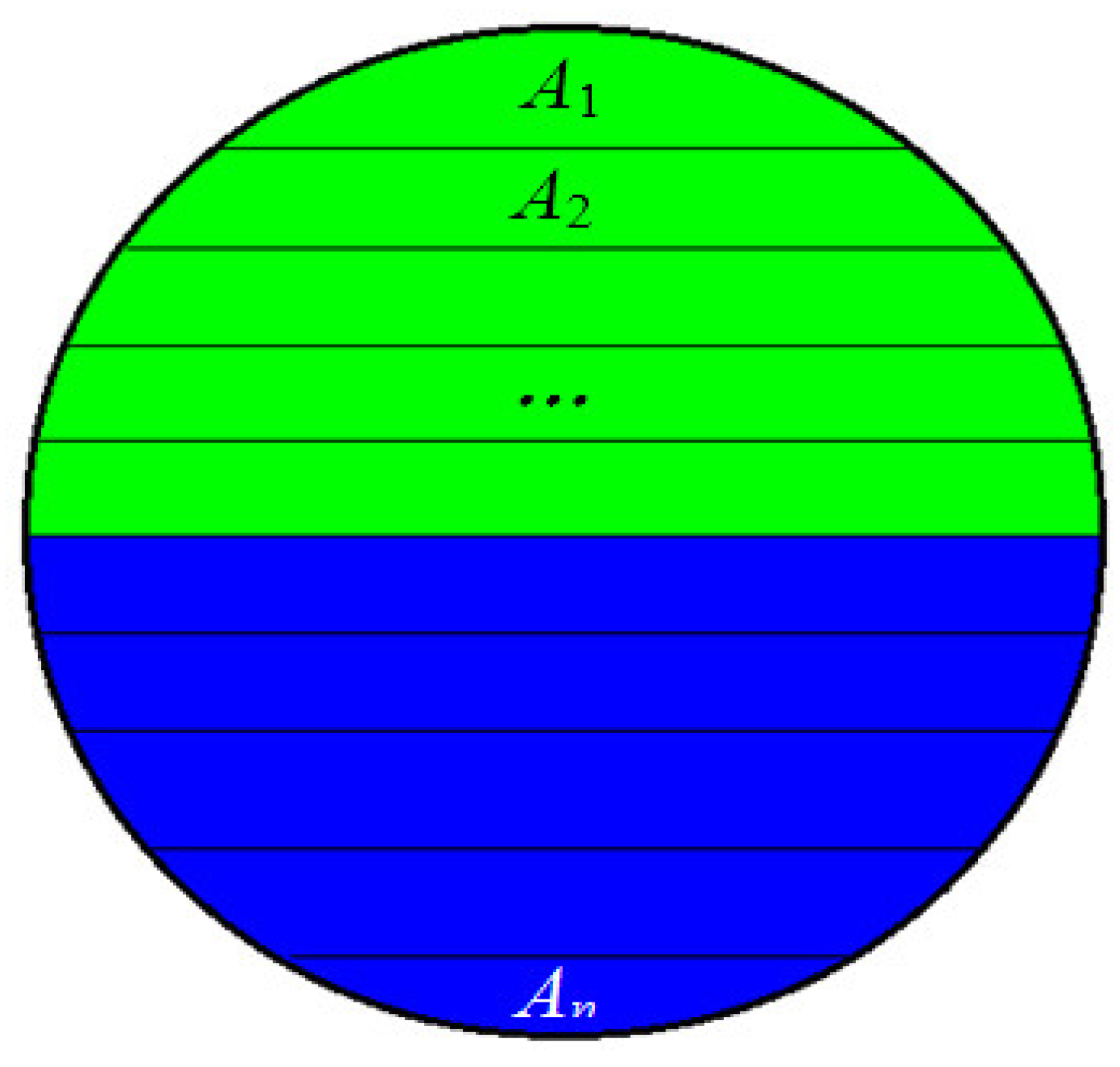
Figure 7 shows the oil–water stratified flow in the near-horizontal well. The wellbore profile is divided into n small profiles of equal height. The cross-sectional area , the water holdup , and the flow velocity in the area where each measurement position was located were obtained for each small profile. The water phase flowrate and oil phase flowrate were also obtained [27].
5. Design of Flow Imaging and Flowrate Interpretation Software
The program in this study was based on the MATLAB environment and used MATLAB’s graphical user interface (GUI), which is a visual software platform. After the program has been designed and completed, the user does not need to modify the design part of the program but only needs to enter the set parameters in the GUI interface. Figure 8 shows the design idea of this program.
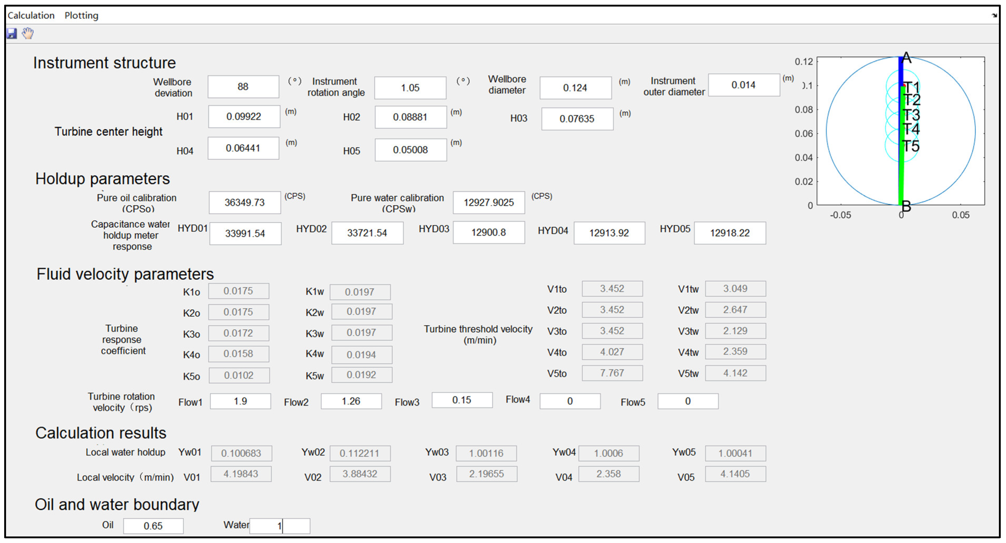
As shown in Figure 9, the first GUI program designed contained five modules. The first module was the tool structure module, which was used to display the position of the turbine and capacitance water holdup meter in the cross section of the wellbore. These values needed to be entered manually based on the measurement data, as these parameters varied for each experimental condition. The second module was the holdup parameters module, which included both the calibration values for the capacitance probe in pure oil and pure water and the capacitance probe response values to be input. When considering the calibration value measured in pure oil and pure water, it was possible to judge whether the fluid was oil or water based on the data measured by the capacitance probe. The third module was the fluid velocity parameters module, which included both the response coefficient and threshold velocity of the turbine in pure oil and pure water, calculated from the above input data, and the actual turbine rotation velocity to be input. The fourth module showed the results of the holdup and flowrate calculations, which was automatically generated based on the above data. The fifth module was the oil–water boundary, which was used to determine oil and water in the holdup profile imaging and needed to be manually input according to the experimental situation.
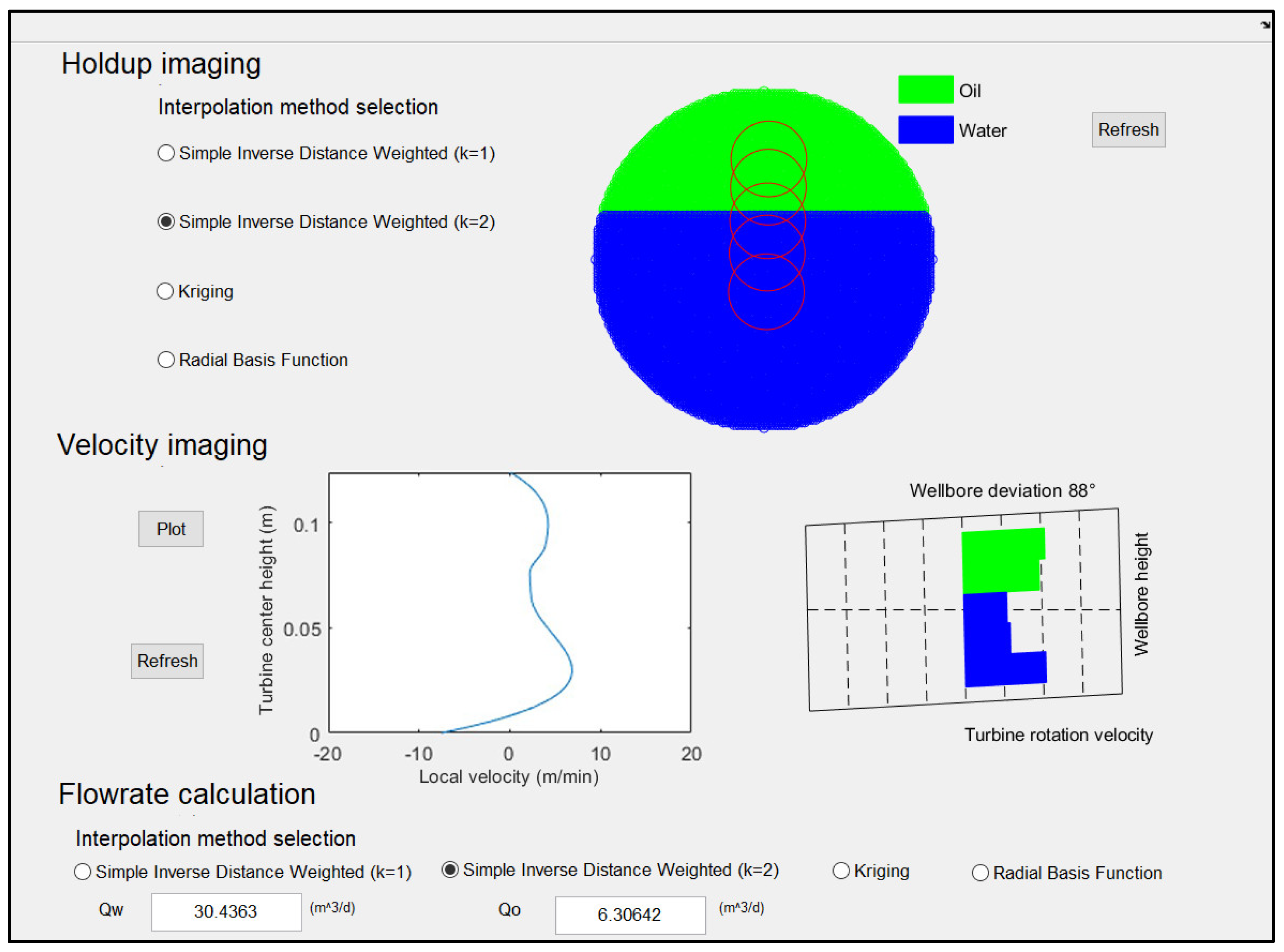
As shown in Figure 10, the second GUI program was used for the calculation of the holdup profile imaging, flow velocity profile imaging, and flowrate of each phase, and the data used in this interface came from the first GUI program. We simply selected the appropriate algorithm, and the image and calculation results were automatically generated.
Overall, the data to be entered were the well deviation angle, angle of rotation of the instrument, height of the turbine center, water holdup meter response value, and rotation velocity of the turbine. The program then calculated the local water holdup, local velocity, and flowrate of each phase, as well as imaging the turbine’s position in the wellbore, the holdup profile, and the flow velocity profile.
6. Discussion of Experimental Data Flow Imaging Results
6.1. Holdup Imaging
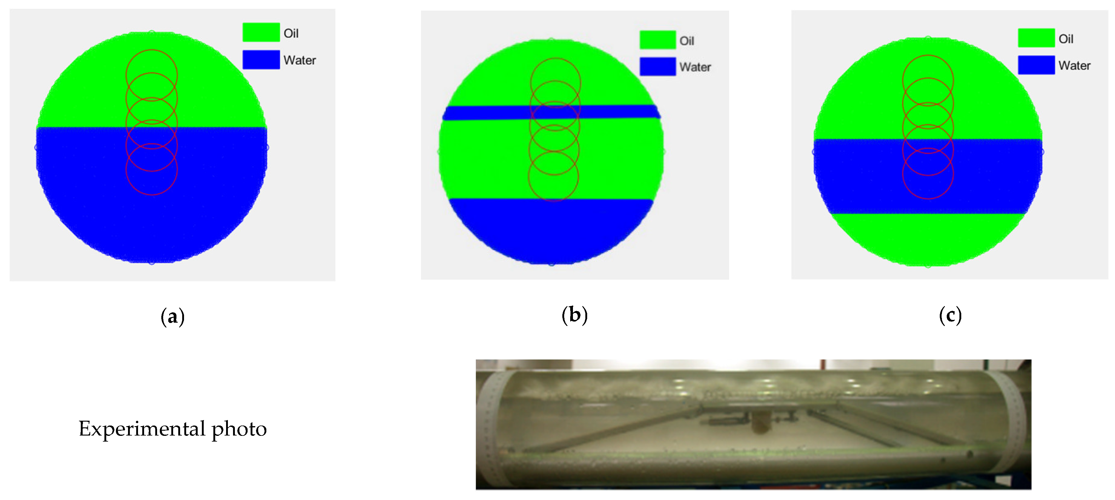
As shown in Figure 11, the local holdup information at five different positions was combined with three interpolation algorithms (inverse distance weight interpolation, radial basis function interpolation, and Kriging interpolation) to obtain the holdup imaging for the specific well deviation angle, flowrate, and water cut conditions [28,29]. By comparing with the experimental flow pattern, it could be judged whether the capacitance holdup imaging effect was consistent with the experiment. It can be seen that when the well deviation angle was 88 degrees, the total oil-water flowrate was 50 , and the water cut was 20%, the imaging effect of the inverse distance weight interpolation method was consistent with the experimental photos.
As shown in Figure 12, by using one-dimensional segmented cubic interpolation, the flow velocity profile imaging could be obtained for a horizontal well at 90°, total flowrate of 120 , and water cut of 40%. The local velocities at five different positions (i = 1–5) were 3.235, 2.669, 2.44, 2.661, and 5.382 m/min.
6.2. Analysis of Flow Imaging Effect
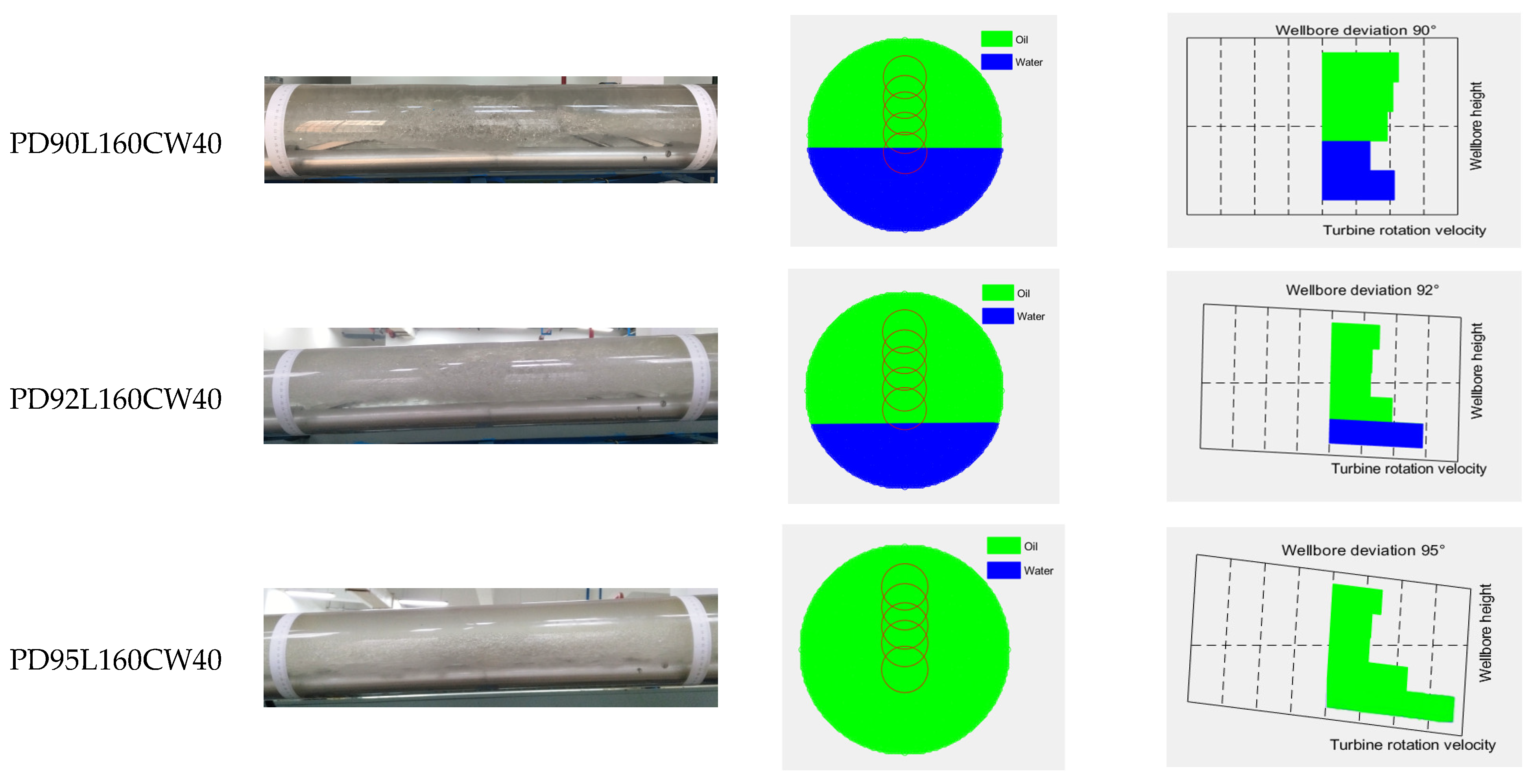
Figure 13 shows the comparison and analysis results of holdup imaging, velocity imaging, and experimental photos under the same total oil–water flowrate, same water cut, and different wellbore deviation angles. It can be seen that light-phase oil and heavy-phase water were distributed at the top and bottom of the wellbore, respectively. However, when the well deviation was on an uphill flow (85° and 88°) due to the large weight of heavy-phase water in the direction of gravity, water accounted for a large proportion of the wellbore cross section, and the water holdup value was too large, greater than 40% of the cross-sectional area of the wellbore. When the well deviation was on a downhill flow (92° and 95°) due to the large weight of heavy-phase water in the direction of gravity, water accounted for a small proportion of the wellbore cross section, and the water holdup value was too small, less than 40% of the cross-sectional area of the wellbore. Since the first measuring point of the lowest height was relatively high in vertical height, it was still in the oil when the wellbore deviation angle was 95°. It could measure the signal of the oil but could not identify the water at the wellbore bottom. Therefore, the SPFI instrument lost its ability to identify water in this case.
7. Discussion of Experimental Data Flow Imaging Results
When the wellbore deviation angles were 85°, 88°, and 90°, the oil–water total flowrate was 50 , and only the water cut changed. The above-mentioned stratified flow flowrate calculation model (Equations (6) and (7)) was used to calculate the oil flowrate, water flowrate, and oil–water total flowrate. Figure 14 shows that the flowrates of each phase calculated by the model were in good agreement with the flowrates of each phase designed in the experiment. At the same time, Table 3 shows that oil–water total flowrate calculated by the model was also in good agreement with the experimental design, and the relative error was within ±6%, indicating that the stratified flow flowrate calculation model has good applicability.
8. Conclusions and Recommendations
(1) On the multi-phase flow simulation device, a single-probe multi-position measurement fluid imager was used to conduct five kinds of simulation experiments with different wellbore deviation angles. The experimental flow patterns under the oil–water flow in near-horizontal wells in this study were mainly smooth stratified flow and wavy stratified flow.
(2) The calculation of local water holdup was carried out based on the collected experimental data combined with the calibration values of pure oil and pure water. At the same time, the calculation of the local velocity was carried out and combined with the response coefficients of turbine instruments for pure oil and pure water. Using the MATLAB language, a processing program was written to realize two-dimensional holdup imaging and velocity imaging.
(3) Based on the calculation model of the flowrate of each phase of the stratified flow, the total flowrate of oil and water was calculated in the case of low-flow stratified flow and compared with the total flow set in the experiment. The results indicated that the relative error was relatively small.
(4) In this paper, an SPFI instrument was used to conduct oil–water flow experiments, and algorithms were used to calculate and process the collected data. The calculation and imaging of velocity and holdup were realized, as well as the flowrate calculation, and the corresponding program was designed in MATLAB. The instrument and software can be applied to field logging in the future to obtain well production and oil–water distribution information.
Author Contributions
Data curation, J.L., S.S. and H.C.; writing—original draft preparation, J.L.; writing—review and editing, J.L. and S.S. All authors have read and agreed to the published version of the manuscript.
Funding
This paper is supported by the National Natural Science Foundation of China (No. 42174163), the Open Fund of Key Laboratory of Exploration Technologies for Oil and Gas Resources (Yangtze University), and the Ministry of Education (Grant No. K2018-10).
Institutional Review Board Statement
Not applicable.
Informed Consent Statement
Not applicable.
Data Availability Statement
Data are contained within the article.
Conflicts of Interest
The authors declare no conflict of interest.
References
- Guo, H.M.; Song, H.W.; Liu, J.F. Production Logging Principles and Data Interpretation, 2nd ed.; Petroleum Industry Press: Beijing, China, 2021. [Google Scholar]
- Bian, X.H.; Liu, J.F.; Ye, T.M.; Zheng, Z.C.; Xu, Z.; Cai, H.T. Numerical Simulation of Oil-water Two-phase Flow Pattern in Large Diameter and Different Inclined Wells. Well Logging Technol. 2016, 40, 399–403. [Google Scholar] [CrossRef]
- Liu, J.F.; Guo, H.M.; Peng, Y.P.; Wang, J.Y.; Xue, W. Experimental Study of Flow Behaviors for Oil-water Two-phase in Large Diameter Horizontal Pipe. J. Oil Gas Technol. 2012, 34, 90–93. [Google Scholar] [CrossRef]
- Bohari, M.; Ali, M.; de Leeuw, H.; Nilsson, C. Multiphase Flow Measurement Using Tracer Technology at Dulang Oil Field, Malaysia. In Proceedings of the SPE Asia Pacific Oil and Gas Conference and Exhibition, Jakarta, Indonesia, 9–11 September 2003. [Google Scholar] [CrossRef]
- Hogendoorn, J.; Boer, A.; Bousche, O.; Zoeteweij, M.; Appel, M.; de Jong, H.; de Leeuw, R. Magnetic Resonance Technology: An Innovative Approach To Measure Multiphase Flow. In Proceedings of the 9th North American Conference on Multiphase Technology, Banff, AB, Canada, 11–13 June 2014. [Google Scholar]
- Baldauff, J.; Eunge, T.; Cadenhead, J.; Faur, M.; Marcus, R.; Mas, C.; Oddie, G. Profiling and Quantifying Complex Multiphase Flow. Oil Field Rev. 2004, 16, 4–13. [Google Scholar]
- Vu-Hoang, D.; Faur, M.; Marcus, R.; Cadenhead, J.; Besse, F.; Haus, J.; Di-Pierro, E.; Wadjiri, A.; Gabon, P.; Hofmann, A. A Novel Approach to Production Logging in Multiphase Horizontal Wells. In Proceedings of the SPE Annual Technical Conference and Exhibition, Houston, TX, USA, 26–29 September 2004. [Google Scholar]
- Cao, Y.Q.; Cao, Y. Research and Application Prospect of Multiphase Flow Measurement Technology. Petrochem. Ind. Technol. 2016, 23, 269–272. [Google Scholar] [CrossRef]
- Zheng, Y.J.; Ma, Y.X.; Zeng, T.; Pan, Y.Z.; Zhao, J.L. Review of Downhole Multiphase Flow Measurement Techniques. Technol. Superv. Pet. Ind. 2016, 32, 31–34. [Google Scholar]
- Wu, Y.; Jiang, A.M. Research on Response Characteristics of Turbine Flowmeter. World Well Logging Technol. 2014, 3, 60–61. [Google Scholar]
- Wang, Z. Research on the Performance of Turbine Flowmeter under Different Fluid Conditions. Ph.D. Thesis, Tianjin University, Tianjin, China, 2008. [Google Scholar]
- Gok, I.M.; Thanh, T.H.; Khunaworawet, T.; Mukerji, P.; Kim, Y.S.; Lee, J.; Sun, D.; Van An, P. Accurate Production Logging in Deviated Gas-Liquid Producer Wells. In Proceedings of the Offshore Technology Conference, Kuala Lumpur, Malaysia, 22–25 March 2016. [Google Scholar]
- Zou, S.L.; Yang, J.X.; Hu, Z.G.; Zhang, Y.; Ni, F.J. Application of FSI Production Profile Logging Technique in Fuling Shale Gas Field. Well Logging Technol. 2016, 40, 209–213. [Google Scholar]
- Ahmad, N.A.; Chieng, Z.H.; Jelie, A.; Abdul Rahman, H.; Amin, M.F.M.; Foo, N.K.H.; Zakeria, A.F.; Sidek, S.; Yahya, F.; Ramli, S.; et al. Array Production Survey Accurately Pinpoints Water Shut-Off Location and Strengthen the Understanding on Remaining Potential of a Giant Carbonate Gas Field, Offshore East Malaysia. In Proceedings of the SPE/IATMI Asia Pacific Oil & Gas Conference and Exhibition, Virtual, 12–14 October 2021. [Google Scholar]
- Younis, A.; Alshehhi, M.; Al Braik, H.; Uematsu, H.; El-Sayed, M.; Manzar, M.A.; Ismail, M.; More, M. Overcoming Production Logging Challenges in Evaluating Extended Reach Horizontal Wells with Advanced Completions. In Proceedings of the Abu Dhabi International Petroleum Exhibition & Conference, Abu Dhabi, United Arab Emirates, 15–18 November 2021. [Google Scholar]
- Yang, R. Study of MAPS Holdup Imaging Processing Method. Ph.D. Thesis, Yangtze University, Jingzhou, China, 2016. [Google Scholar]
- Liao, L.; Zhu, D.; Yoshida, N.; Hill, A.D.; Jin, M. Interpretation of Array Production Logging Measurements in Horizontal Wells for Flow Profile. In Proceedings of the SPE Annual Technical Conference and Exhibition, New Orleans, LA, USA, 30 September–2 October 2013; p. 166502. [Google Scholar] [CrossRef] [Green Version]
- Dejia, D.; Wei, P.; Jun, M.; Shuang, A.; Ying, H. Production Logging Application in Fuling Shale Gas Play in China. In Proceedings of the SPE Asia Pacific Oil & Gas Conference and Exhibition, Perth, Australia, 25–27 October 2016. [Google Scholar]
- Smolen, J.J. Cased Hole and Production Log Evaluation; PennWell Publishing Company: Tulsa, OK, USA, 1996. [Google Scholar]
- Hill, A.D. Production Logging: Theoretical and Interpretive Elements; HL Doherty Memorial Fund of AIME, Society of Petroleum Engineers: Richardson, TX, USA, 1990. [Google Scholar]
- Trallero, J.L.; Sarica, C.; Brill, J.P. A Study of Oil-water Flow Pattern in Horizontal Pipes. SPE Prod. Facil. 1996, 12, 165–172. [Google Scholar] [CrossRef]
- Zong, Y.B. Measurement of the Properties of Oil-Water Two-Phase Flow in Inclined and Horizontal Pipes. Ph.D. Thesis, Tianjin University, Tianjin, China, 2009. [Google Scholar]
- Zhan, L.N. Study on the Flow Law of Oil-Water Two-Phase Horizontal Pipe. Ph.D. Thesis, Southwest Petroleum University, Chengdu, China, 2005. [Google Scholar]
- Huang, Y.T.; Ding, J.; Li, H.; Wu, Y.X. Study of oil-water two-phase flow pattern characteristic using electrical resistance tomography technology. Chin. J. Hydrodyn. 2015, 30, 70–74. [Google Scholar]
- Li, Z.C.; Fan, C.L. A novel method to identify the flow pattern of oil–water two-phase flow. J. Pet. Explor. Prod. Technol. 2020, 10, 3723–3732. [Google Scholar] [CrossRef]
- Zhang, D.L.; Zhang, H.B.; Rui, J.W.; Pan, Y.X.; Liu, X.B.; Shang, Z.P. Prediction model for the transition between oil-water two-phase separation and dispersed flows in horizontal and inclined pipes. J. Pet. Sci. Eng. 2020, 192, 107161. [Google Scholar] [CrossRef]
- Li, Q.Z.; Liu, J.F.; Gao, F.; Dai, Y.X.; Peng, W.S. Interpretation Method of Oil-Water Two-Phase Flow in Horizontal Well Based on Array Spinner and Array Holdup Tools. Well Logging Technol. 2021, 45, 405–410. [Google Scholar] [CrossRef]
- Liu, J.F.; Xu, Y.C.; Wu, Q.X. Holdup flow imaging analysis for capacitance and resistance ring array probes. Prog. Geophys. 2018, 33, 2141–2147. [Google Scholar] [CrossRef]
- Cui, S.F.; Liu, J.F.; Li, K.; Li, Q.Z. Data Analysis of Two-Phase Flow Simulation Experiment of Array Optical Fiber and Array Resistance Probe. Coatings 2021, 11, 1420. [Google Scholar] [CrossRef]
Figure 1.
Schematic diagram of multi-phase flow simulation device for horizontal and high-angle deviated well. 1–2. A simulated wellbore (inner diameter of 124 mm), 3–4. B simulated wellbore (inner diameter of 159 mm), 5. Experimental observation site, 6. Oil–water four-stage separation tanks, 7. Oil tank, 8. Oil pump, 9. Oil flow meters, 10. Oil control valves, 11. Water tank, 12. Water pump, 13. Water flow meters, 14. Water control valves, 15. Oil–water mixer. Yellow represents oil, and blue represents water.

Figure 2.
Schematic diagram of single-probe multi-position measurement fluid imager (SPFI).

Figure 3.
Diagram of measurement points.

Figure 4.
Schematic diagram of experimental flow patterns at different wellbore deviation angles. PD represents wellbore deviation angle; (a) OW-PD85; (b) OW-PD92; (c) OW-PD90; (d) OW-PD92; (e) OW-PD95.
Figure 4.
Schematic diagram of experimental flow patterns at different wellbore deviation angles. PD represents wellbore deviation angle; (a) OW-PD85; (b) OW-PD92; (c) OW-PD90; (d) OW-PD92; (e) OW-PD95.

Figure 5.
Diagram of measurement points.

Figure 6.
Single-phase (pure water) turbine response (different wellbore deviation angles, same measuring point height).
Figure 6.
Single-phase (pure water) turbine response (different wellbore deviation angles, same measuring point height).

Figure 7.
Schematic diagram for calculating flowrate.

Figure 8.
The design idea of the program.

Figure 9.
The GUI program and calculation results.

Figure 10.
The second GUI program and calculation results.

Figure 11.
Smooth stratified flow holdup imaging (OW-PD88L50CW20); (a) Inverse distance weight interpolation; (b) Radial basis function interpolation; (c) Kriging interpolation.
Figure 11.
Smooth stratified flow holdup imaging (OW-PD88L50CW20); (a) Inverse distance weight interpolation; (b) Radial basis function interpolation; (c) Kriging interpolation.

Figure 12.
Velocity profile imaging (PD90L120CW40).

Figure 13.
Comparison of flow imaging effects at the same flowrate, same water cut, and different wellbore deviation angles (L160CW40).
Figure 13.
Comparison of flow imaging effects at the same flowrate, same water cut, and different wellbore deviation angles (L160CW40).


Figure 14.
Calculated oil and water flowrate consistency analysis diagram.


Table 1.
Trallero et al.’s horizontal-pipe oil–water flow pattern classification. OW represents the oil-water, PD represents the wellbore deviation angle, L represents the total flowrate of oil and water, and CW represents the water cut.
Table 1.
Trallero et al.’s horizontal-pipe oil–water flow pattern classification. OW represents the oil-water, PD represents the wellbore deviation angle, L represents the total flowrate of oil and water, and CW represents the water cut.
| Flow Pattern Classification | Schematic Diagram | Experimental Photo (OW-PD90) | ||
|---|---|---|---|---|
| Stratified flow | Smooth stratified flow |  |  L50CW20 | |
| Wavy stratified flow |  |  L100CW60 | ||
| Dispersed flow | Water-phase dominated | Oil in water and water |  |  L120CW80 |
| Oil in water |  |  L200CW20 | ||
| Oil-phase dominated | Water in oil and oil in water |  | ||
| Water in oil |  | |||
Table 2.
Local water holdup at different positions (OW-PD90L50CW20).
| Position of Measuring Points | Height of Measuring Points (mm) | Capacitance Water Holdup Response (CPS) | Pure Oil Response (CPS) | Pure Water Response (CPS) | Calculated Local Water Holdup |
|---|---|---|---|---|---|
| 1 | 100 | 34,367.48 | 36,349.73 | 12,927.91 | 0.085 |
| 2 | 88 | 34,428.84 | 0.082 | ||
| 3 | 76 | 34,390.53 | 0.084 | ||
| 4 | 64 | 34,259.53 | 0.089 | ||
| 5 | 48 | 15,250.64 | 0.901 |
Table 3.
Comparison between experimental and model-calculated total flowrate.
| Wellbore Deviation Angle | Experiment Total Flowrate (m3/d) | Water Cut (%) | Calculated Total Flowrate (m3/d) | Relative Error (%) |
|---|---|---|---|---|
| PD85 | 50 | 20 | 49.584 | −0.83 |
| 50 | 40 | 47.851 | −4.3 | |
| 50 | 50 | 47.847 | −4.3 | |
| 50 | 60 | 51.817 | +3.6 | |
| 50 | 70 | 51.304 | +2.6 | |
| 50 | 80 | 48.695 | −2.6 | |
| 50 | 90 | 52.213 | +4.4 | |
| PD88 | 50 | 20 | 52.635 | +5.3 |
| 50 | 40 | 48.025 | −4.0 | |
| 50 | 50 | 47.649 | −4.7 | |
| 50 | 60 | 49.336 | −1.3 | |
| 50 | 70 | 49.082 | −1.8 | |
| 50 | 80 | 48.434 | −3.1 | |
| 50 | 90 | 52.892 | +5.8 | |
| PD90 | 50 | 20 | 47.982 | −4.2 |
| 50 | 40 | 47.014 | −6.0 | |
| 50 | 50 | 47.664 | −4.6 | |
| 50 | 60 | 47.630 | −4.7 | |
| 50 | 70 | 50.734 | +1.5 | |
| 50 | 80 | 50.653 | +1.3 | |
| 50 | 90 | 51.744 | +3.5 |
Publisher’s Note: MDPI stays neutral with regard to jurisdictional claims in published maps and institutional affiliations. |
© 2022 by the authors. Licensee MDPI, Basel, Switzerland. This article is an open access article distributed under the terms and conditions of the Creative Commons Attribution (CC BY) license (https://creativecommons.org/licenses/by/4.0/).
Share and Cite
MDPI and ACS Style
Liu, J.; Shi, S.; Chen, H. Experimental Research on Oil–Water Flow Imaging in Near-Horizontal Well Using Single-Probe Multi-Position Measurement Fluid Imager. Processes 2022, 10, 1051. https://doi.org/10.3390/pr10061051
AMA Style
Liu J, Shi S, Chen H. Experimental Research on Oil–Water Flow Imaging in Near-Horizontal Well Using Single-Probe Multi-Position Measurement Fluid Imager. Processes. 2022; 10(6):1051. https://doi.org/10.3390/pr10061051
Chicago/Turabian StyleLiu, Junfeng, Shoubo Shi, and Hang Chen. 2022. "Experimental Research on Oil–Water Flow Imaging in Near-Horizontal Well Using Single-Probe Multi-Position Measurement Fluid Imager" Processes 10, no. 6: 1051. https://doi.org/10.3390/pr10061051
Note that from the first issue of 2016, this journal uses article numbers instead of page numbers. See further details here.