

Reservoir Advanced Process Control for Hydroelectric Power Production

1
Dipartimento di Ingegneria dell’Informazione, Università Politecnica delle Marche, Via Brecce Bianche 12, 60131 Ancona, Italy
2
Alperia Green Future, 60015 Falconara Marittima, Italy
*
Author to whom correspondence should be addressed.
Processes 2023, 11(2), 300; https://doi.org/10.3390/pr11020300
Submission received: 29 November 2022
/
Revised: 5 January 2023
/
Accepted: 12 January 2023
/
Published: 17 January 2023
(This article belongs to the Special Issue Automation Control Systems & Process Control for Industry 4.0)
Abstract
:The present work is in the framework of water resource control and optimization. Specifically, an advanced process control system was designed and implemented in a hydroelectric power plant for water management. Two reservoirs (connected through a regulation gate) and a set of turbines for energy production constitute the main elements of the process. In-depth data analysis was carried out to determine the control variables and the major issues related to the previous conduction of the plant. A tailored modelization process was conducted, and satisfactory fitting performances were obtained with linear models. In particular, first-principles equations were combined with data-based techniques. The achievement of a reliable model of the plant and the availability of reliable forecasts of the measured disturbance variables—e.g., the hydroelectric power production plan—motivated the choice of a control approach based on model predictive control techniques. A tailored methodology was proposed to account for model uncertainties, and an ad hoc model mismatch compensation strategy was designed. Virtual environment simulations based on meaningful scenarios confirmed the validity of the proposed approach for reducing water waste while meeting the water demand for electric energy production. The control system was commissioned for the real plant, obtaining significant performance and a remarkable service factor.
1. Introduction
In hydroelectric power plants, maximizing the efficiency of water exploitation is a major challenge for a profitable energy production. This challenge is part of the more general context aimed at minimizing water waste [1,2,3]. Over the past decades, hydropower equipment has been optimized to achieve high performance, availability, and flexibility; these improvements contribute to the energy transition [4,5,6,7]. Hydroelectric power plants may include different sub-processes, e.g., water collection reservoirs, regulation gates, intakes, rivers, sand traps, turbines, floodgates. Digitalization is playing a key role in improving the efficiency of hydropower plants at different levels of the control/automation hierarchy [8]. In this context, advanced process control (APC) systems [9], optimization algorithms [10], and Industry 4.0 [11] can represent strategic solutions. In order to design APC systems and optimization algorithms for non-standard processes and to apply Industry 4.0 principles, suitable cross-fertilization procedures are needed so as to adapt the smart solutions to the considered case studies [12,13]. Adapting APC, high-level optimization, and Industry 4.0 solutions developed in industrial plants to the field of hydropower requires a methodological approach that takes into account the different hardware and software architectures. APC systems can represent software solutions for improving the conduction of hydropower plants and standardizing control operations in the field. In this way, plant operators can play a role at the supervisory level. The benefits offered by APC systems increase as the complexity of the process increases. The complexity of the process includes several aspects, such as the number of variables involved, the types of relationship between the different variables, and the need for predictive approaches [8,14,15]. Industry 4.0 principles can represent strategic drivers of data exchange between the different levels of the automation hierarchy, while optimization algorithms at high levels of automation are able to take into account overall plant benefits—for example, considering the market prices of electric energy [10]. In the literature, many engineers, researchers, and practitioners have tackled optimization, estimation, and control challenges for hydroelectric power plants.
High-level optimization problems were tackled in [10,16,17,18,19,20,21,22]. In [10], a review of optimization algorithms in solving hydro-generation scheduling problems is presented; long-, mid-, and short-term hydro scheduling problems are analyzed, and the target of optimizing the power generation schedule of the accessible hydropower units is presented. Different solutions are detailed, e.g., metaheuristic optimization methods. In [16], the generation scheduling problem, i.e., the unit commitment problem, is investigated through the optimization of the amount of energy that must be provided by each turbine generator. Different versions of the coral reefs optimization algorithm are exploited. In [17], the implementation of reservoir conduction rules using inter-basin water transfer is proposed, and an optimization model based on network flow and particle swarm optimization is adopted for the maximization of the hydroelectric benefits. In [18], the problem of long-term maximization of hydroelectric energy generation from complex multipurpose reservoir systems is solved. The maximization of energy production is the main objective, and genetic algorithms are exploited for the solution of the formulated optimization problems in different scenarios. In [19], a model for a reservoir system is proposed in order to design optimized strategies for the minimization of raw water production cost, the maximization of electrical energy production, and to prevent flood situations. In [20], the authors focus on joint operation and dynamic control of flooding to limit the water level for cascade reservoirs. An effective tradeoff between the flood control and hydropower generation is provided. In [21], a salp swarm algorithm is used to optimize the joint operation of multiple hydropower reservoirs. Multiple strategies combining sine–cosine operators, opposition-based learning mechanisms, and elitism strategies are applied, and the proposed approach is tested through simulations. In [22], optimal operation of reservoirs for power generation plants is proposed. The formulation and implementation of optimal operation schemes are improved by combining the advantages of conventional and optimal operation and using the concept of a warning water level in the operational rules. Calculation under different operating conditions is used to test the developed procedures on a simulated hydropower station.
APC systems for the energy generation devices of hydropower plants are proposed in [23,24,25,26]. In [23], a method for controlling the real power delivered by a hydroelectric power plant to a local electrical grid is proposed, based on advanced control techniques, where internal model control and feedforward strategies are combined. Furthermore, a control loop for the frequency correction is added, a tuning method for the controller is proposed, and the designed controller is tested through simulations. In [24], the problem of load distribution between hydraulic units is tackled. The nonlinearity of the hydro turbine characteristics, individual peculiarities of the generation units, and process constraints are taken into account. A field experiment is executed to test the proposed algorithms. In [25], the hydraulic turbine’s governing system control problem is analyzed; a nonlinear model is proposed, and Takagi–Sugeno fuzzy linearization and mixed H2/H∞ robust control theory are applied to design the controller. The developed APC system is tested through simulations. In [26], modeling and simulation of hydropower plants is assessed in order to test different structures and algorithms for power, frequency, and voltage control. The dynamic and stationary behavior of the hydro units is analyzed in order to implement digital control algorithms.
The high-level optimization algorithms reported in previous studies do not govern the management of the real-time operation of the plants, while the aforementioned APC systems are focused on the control of the energy generation devices. APC systems focused on reservoirs’ and tanks’ level/volume control are proposed in [27,28,29,30,31,32,33,34,35,36] instead. Estimation and control problems are assessed in [27] for water-level control in reservoirs through floodgate manipulation. A nonlinear model predictive control (MPC) with an extended Kalman filter is the solution proposed by the authors, which is tested through simulations. In [28], a system of three interconnected tanks is modeled through Takagi–Sugeno fuzzy models, and a systematic control design procedure is proposed in order to include constraints on the input/output in the formulation. A bank of linear controllers is designed, and linear matrix inequalities are exploited. The proposed procedure is tested through simulations. In [29], a predictive functional control approach is proposed for a three-tank system showing the potential of a predictive controller equipped with an anti-wind-up method through simulations. In [30], an MPC approach is proposed for controlling river systems with water reservoirs, where the main control objective is avoiding the risk of flooding; simulation results are provided for the testing of the designed controller. In [31], five distributed MPC schemes using a hydropower plant benchmark are compared, and specific simulation results are provided; the main objective of the controllers is the coordination of several subsystems over a large geographical area in order to produce the demanded energy while satisfying constraints on water levels and flows. In [32], generalized predictive control is applied to a multivariable model of a pumped-storage hydroelectric power station. The response of the system with constrained predictive control is compared with the existing proportional–integral controller through simulations, showing the benefits provided by MPC. In [33], a predictive control strategy is presented for a process represented by two liquid tanks with a flow control valve. Modelization, control, and disturbance rejection topics are analyzed through simulations. An approach to optimal hydraulic-level tracking based on an inverse optimal controller is proposed in [34], devised with the purpose of regulating power generation rates in a specific hydropower infrastructure. In addition, a neural network is implemented to aid the system in the prediction and management of external perturbations, and the proposed approach is tested through simulations using data collected from the plant throughout a whole year of operation as a tracking reference. A multi-objective MPC approach is presented in [35] for real-time operation of a multi-reservoir system. The approach incorporates the non-dominated sorting genetic algorithm II (NSGA-II), multi-criteria decision-making, and the receding horizon principle to solve a multi-objective reservoir operation problem in real time. The control objectives are to minimize the storage deviations in the reservoirs, to minimize flood risks at a vulnerable downstream location, and to maximize hydropower generation. Tailored simulations are used for the testing of the designed control system. In [36], a six-dimensional nonlinear hydropower system controlled by a nonlinear predictive control method is proposed; a performance index with a terminal penalty function is selected, and numerical experiments are used to test the developed control strategy.
The present paper proposes an APC system aimed at water management for reservoirs in a hydroelectric power plant. Two reservoirs (connected through a regulation gate) and a set of turbines for energy production constitute the main elements of the process. This paper aims to provide holistic knobs and solutions for the assessment of the previously cited aspects of APC systems for hydropower plants. The present paper extends the contents reported in [37], providing additional details and insights on the different phases of the developed project. To the best of the authors’ knowledge, in the literature on APC systems in hydropower plants focused on reservoirs’ level/volume control, the following aspects have not been explored in depth:
- The procedures for a qualified plant inspection before starting an APC project have not been thoroughly detailed in the literature. The selection, acquisition, storage, and analysis of data play a fundamental role in the plant inspection, together with a detailed study of the plant’s devices.
- A detailed feasibility study on the application of MPC for controlling hydropower plants is not present in the literature. Modelization and forecasting need to be assessed in this phase, together with tailored strategies for model mismatch compensation.
- A procedure that defines the MPC constraints, reference trajectories, and tuning parameters in real time based on current and predicted process conditions is not present in the literature on hydropower plants.
- An APC system that takes into account bad data detection, local control loop malfunctions, and lack of efficiency flags in real time is not present in the literature on hydropower plants.
- Smart alarm assessment for hydroelectric power plants is not present in the literature. Smart alarms can represent useful tools during plant conduction, highlighting inefficiency and/or predicting potential problems.
In addition, to the best of the authors’ knowledge, projects on hydropower plants that include implementation of real processes that are designed as lasting control applications and not as temporary tests are not widespread. The field application of an APC system designed and tested through virtual environment simulations requires significant reliability and robustness in order to bridge the gap between simulations and field application.
The remainder of this paper is organized as follows: The Section 2 reports the process description, the control specifications, and the data analysis and modelization methods. In addition, the APC design, the field implementation, and the computational framework are described. The Section 3 focuses on data analysis, modelization, forecasting, virtual environment simulations, and field results. Finally, some conclusions and insights for future work are reported.
2. Materials and Methods
2.1. Process Description, Control Specifications, and Project Definition
The studied process is represented by a hydroelectric power plant located in the Alto Adige region (Italy). Figure 1 shows the geographic characterization of the overall plant. Two artificial water collection reservoirs characterize the process: an upstream reservoir and a downstream reservoir. The downstream reservoir is located in a valley. At the outlet of the downstream reservoir, a tunnel (see Figure 1) takes the water towards a penstock that leads to the power plant (see Figure 2). The electric energy is generated by the rotation of the involved turbines. The water flow between the two reservoirs is controlled through a regulation gate, named the Beikircher gate (see Figure 1). The regulation gate, activated by a butterfly valve, controls the water flow of a pipeline connecting the two reservoirs. The overall process is schematically reported in Figure 3.
The power plant is characterized by a double group of Francis-type turbines capable of providing an overall efficient power of 22 MW and an average annual electric energy production of 86.81 GWh. In the water catchment area, different rivers are present (see Figure 1). As shown in Figure 3, the reservoirs are characterized by two inlet water flows and one outlet water flow. The reservoirs’ level and inlet/outlet water flow rates are measured by suitable sensors. The water flows entering the upstream reservoir consist of the main stream of a river from the intake structure and a set of subsidiary intakes (see Figure 3). Through two side-by-side deicing tanks and two subsequent sand traps, the incoming water from the intake structures flows into the upstream reservoir. The maximum derivable flow rate from the intake structure with clean grids is equal to about 9 m3/s. On the other hand, the subsidiary intakes can provide a maximum flow rate equal to 1.4 m3/s. The two inlet water flows of the upstream reservoir are measured by a level transducer located near the reservoir inlet.
The upstream reservoir was constructed on the right bank of a river and has a maximum length of 280 m and a maximum width of 150 m, with a usable capacity of about 135,500 m3. The bottom level of the reservoir is at 1216 m above sea level (asl), while the overflow level is 1223.60 m asl. The minimum level detectable by the level sensor is 1216.80 m asl; below this level, the operation of the upstream reservoir has to be considered run-of-river. The maximum detectable level is equal to about 1221.85 m. At the outlet of the upstream reservoir, the Beikircher gate regulates the water flow, which enters a tunnel. The length of the tunnel that connects the upstream and downstream reservoirs is equal to 5534 m. The butterfly valve of the regulation gate is controlled by a built-in programmable logic controller (PLC). A hydraulic control unit, placed in a structure near the valve, operates the gate. The flow rate setpoint can be manipulated between 0 and 8 m3/s. According to the plant’s needs, the maximum value is typically limited to 7 m3/s. The downstream reservoir was constructed on the right bank of the associated river and has a maximum length of 165 m and a maximum width of 80 m, with a usable capacity of about 52,500 m3. The downstream reservoir’s capacity is lower than the upstream reservoir’s capacity. The downstream reservoir (see Figure 3), similarly to the upstream reservoir, is characterized by two inlet flows and a single outlet flow. The downstream reservoir’s inlet flows are the water flow from the upstream reservoir (regulated by the Beikircher gate) and the intake structure. The intake structure is represented by the water flowing in a gravel reservoir and in a sand trap (see Figure 3). The bottom level of the reservoir is at 1197.20 m asl, while the overflow level is 1203.50 m asl. The minimum level detectable by the level sensor is 1197.40 m asl; below this level, the operation of the downstream reservoir has to be considered run-of-river. The maximum detectable level is equal to about 1202.77 m. At the outlet of the downstream reservoir, the water is conveyed towards the power plant through a tunnel and a penstock. The tunnel is characterized by a length equal to about 7000 m, while the penstock, which consists of a metal pipe, has a length of about 500 m. A jump equal to about 270 m is observed. After passing through the power plant and transferring energy to the turbines, the water flows into a free surface drainage channel, intercepted by two flat gates. The water released by the downstream reservoir is subjected to a flow rate setpoint regulation. The regulation and the flow rate measurement are located not at the outlet of the downstream reservoir, but a few meters downstream. The flow rate regulation is based on the electric energy production plan of the power plant. The electric energy production plan is known a priori with significant confidence. The production plan is sent daily to the managers of the plant and determines how much energy the plant will have to produce hourly during the day. The provided electric power (MW) measurements, together with the related setpoints, are available for the turbines.
Based on tailored plant inspections and plant operators’/managers’ interviews/reports, different considerations were made for the process in order to plan the project phases. A list of the manipulated variables (MVs), controlled variables (CVs), and measured disturbance variables (DVs) was obtained [38]. The flow rate setpoint (m3/s) of the regulation gate represents the only MV for the APC system. The CVs are represented by the volume (m3) of the upstream and downstream reservoirs, while the measured DVs are represented by the remaining water inlet/outlet flow rates (m3/s) reported in Figure 3: the upstream reservoir intake, the subsidiary intakes, the downstream reservoir sand trap, and the outlet flow rate from the downstream reservoir. Measured DVs are manipulated by other controllers or related to the natural flow of rivers. All of the reported MVs and DVs were measured, while the CVs were not directly measured. CVs’ indirect measurement computation was performed using the measurements of the reservoirs’ level.
The previous conduction of the plant was represented by manual and semiautomatic control logics. This conduction was based on empirical laws and experience with the process. The main control specifications were as follows:
- Constrained control of the reservoirs’ volume (level). This type of control is usually referred to as zone control [39].
- Avoid water overflow on the reservoirs: the upstream reservoir has a lower priority than the downstream one, since the downstream reservoir is closer to the town.
- Avoid water shortages in the reservoirs: the downstream reservoir has a higher priority, since a lack of water in downstream reservoir could cause a violation of the electric energy production plan of the hydroelectric power plant.
- Compliance with the physical constraints and with the technical operative constraints of the Beikircher regulation gate.
The zone control strategy, resulting from the first specification, is intended for the constrained control of the reservoirs’ volume (level), respecting the priorities previously reported in [39]. The constraints can help in avoiding water overflow and water shortages, ensuring the safe conduction of the plant. An efficient zone control is not always achievable in the process under study, because only an MV may be available—for example, the inlet flow rates of the upstream reservoir are not manipulable. The electric energy production plan of the hydroelectric power plant must be respected, because a violation (in excess or in deficit) usually causes an economic penalty for the plant [21]. As explained below, the physical constraints are mainly focused on the Torricelli law [23,24,25] and on the effective capacity of the plant devices. The technical operative constraints of the Beikircher regulation gate are intended to avoid (if possible) too-frequent control moves in order to minimize the wear damage. In this context, an automatic APC system for real-time control must guarantee an optimal solution for the flow rate setpoint of the regulation gate (MV) under all process conditions. Furthermore, smart alarms highlighting abnormal plant conditions could improve the plant’s conduction. In this way, plant operators can play roles at a supervisory level. The control specifications and the proposed control strategy are summarized in Figure 4, while Figure 5 reports the main project phases described below. The accurate definition of the inputs and outputs to be obtained in each project phase represents a critical step.
2.2. Data Selection, Acquisition, and Storage
The selection of the process variables to be acquired and stored, together with the definition of the hardware and software architectures to be exploited in real time, was a key phase that required special effort. The plant data were acquired in the field through the PLCs. First, an accurate data selection phase was performed. All MV and measured DV values were selected, together with the reservoirs’ level. Also included in the selected data were variables involved in the lower-level control loops—for example, the process variables of the regulation gate and the downstream reservoir outlet flow rate—and the available process variables of the power plant—for example, the electric power of the turbines. Furthermore, a procedure for the supply of the electric energy production plan was defined.
In order to acquire and store the selected data, a suitable architecture was designed (Figure 6). The selected data were acquired from the plant through the PLCs (PLCs, Figure 6). Furthermore, the high-level supervisory systems provided the electric energy production plan in advance (High-Level Supervisory Systems, Figure 6). A PC server was installed in the plant, and it was connected to the plant’s net infrastructure. On the PC server, a supervisory control and data acquisition (SCADA) system was installed and a database was created (PC Server (SCADA and Database), Figure 6). The data selection, acquisition, and storage procedures were implemented on the PC server. Furthermore, a PC client (Client Control Room, Figure 6) was installed in the control room of the plant in order to provide selected signal information to the plant’s operators, engineers, and managers. Tailored data visualization methods were designed in order to make the provided information user-friendly.
2.3. Data Analysis
Following data selection, acquisition, and storage, data analysis was performed [40,41,42]. The data analysis sub-phases were difficult to define in the present work. The data analysis phase was divided into three main sub-phases:
- Analysis and processing of process variables and setpoints;
- Performance evaluation of local control loops;
- Assessment related to the electric energy production plan data and the compliance with the electric energy production plan.
The sub-phase consisting in the analysis and processing of process variables and setpoints involved the measurement of the process variables by sensors and the setpoints commanded on the local controllers. The sensors’ acquisition/measurement and the PLCs’ communication errors/malfunctions were investigated, and the missing data were replaced on the database by the results of tailored regressions. Suitable data preprocessing techniques (e.g., validity limits and spike and freezing checks) were applied in order to detect the bad data, which were discarded. The validity limits and spike and freezing thresholds were tuned based on the sensors’ data sheets and the historical data. Furthermore, mobile window filters were used to improve the robustness of the selected measurements. The applied mobile window filters had the following form:
where is the discrete-time instant, is the number of samples of the window, represents the sensor measurements, and is the filtered measurement at instant .
The local control loops’ performance evaluation sub-phase consisted of an assessment of the performances of the local controllers of the Beikircher regulation gate and of the downstream reservoir outlet water flow. Some experimental tests were performed consisting of suitable step moves on the gate setpoint, evaluating the rise time, the overshoot, and the settling time. Furthermore, deviation conditions between the setpoints and process variables were investigated [43,44,45]. In order to motivate the potential abnormal behaviors of the local controllers—and especially of the regulation gate controller—the Torricelli law [23,24,25] was exploited:
where is the discrete-time instant, (m3/s) is the maximum reachable value by the regulation gate’s flow rate, (m2) is the pipeline section, (m/s2) is the acceleration of gravity (constant), and (m) is the height of the water level above the reservoir outlet conduct. Equation (2) is derived from the Bernoulli equation [23,24,25]. Table 1 reports the values of the parameters involved in Equation (2) for the regulation gate’s flow rate. The involved pipeline connects the upstream reservoir to the regulation gate, so the water height has to be considered with respect to the level of the upstream reservoir outlet. The minimum level detectable by the upstream reservoir’s level sensor was taken into account, i.e., 1216.80 m (see Table 1). If the upstream reservoir’s level ( in Table 1) is greater than or equal to about 1218.35 m asl, a flow rate of up to 8 m3/s can be required on the regulation gate. If the upstream reservoir’s level is greater than or equal to about 1218 m, a maximum flow rate of up to 7 m3/s can be required on the regulation gate. On the other hand, if the upstream reservoir’s level is lower than the computed thresholds, the physically reachable flow rate setpoint on the regulation gate decreases (see Table 1). For these reasons, as explained in Section 2.7, Equation (2) was also used for real-time modifications of the MV upper constraints.
The electric energy production plan data were evaluated in order to verify the implemented data-exchange procedure between the SCADA and the high-level supervisory systems (see Figure 6). Furthermore, an in-depth verification of the compliance of the defined electric energy production plan was performed.
The previously mentioned data analysis procedures were customized in order to be implemented in the real-time APC system. A module was designed, named Bad Detection, Data Conditioning, and DV Prediction module which, among its functions, includes an ad hoc bad data detection algorithm together with an algorithm that performs data filtering on mobile windows. Furthermore, the local control loops are checked for malfunction and compliance with the electric energy production plan is verified within this module. An overall data analysis reliability flag results from the aforementioned checks. This flag is exploited by the APC system (see Section 2.7); in this way, bad data detection, local control loop malfunctions, and f inefficient conditions are included in the real-time implementation of the APC system.
To the best of the authors’ knowledge, the proposed methods for data selection, acquisition, storage, and analysis represent an innovation in the literature on APC systems for hydropower plants. Not using accurate methods of data selection, acquisition, storage, and analysis may represent a missing key prerequisite for designing a robust APC system.
2.4. Modelization
In order to design an MPC solution for the process under consideration, the modelization is a fundamental requirement, because MPC techniques strictly depend on the goodness of the obtained process model. A linear modelization approach, based on first-principles equations [21,24,46,47] and empirical data-based time delay identification [48], was adopted. The resulting continuous-time model was as follows:
where is the continuous time variable (min), (m3) and (m3) are the upstream and downstream reservoirs’ water volumes, respectively, and (m3/s) is the regulation gate flow rate setpoint. (m3/s) is the upstream reservoir’s intake flow rate, (m3/s) is the upstream reservoir’s subsidiary intakes’ flow rate, (m3/s) is the downstream reservoir’s sand trap inlet flow rate, and (m3/s) is the downstream reservoir’s outlet flow rate (see Figure 3). In Equations (3) and (4), note the sign of each term—the inlet flow rates have a positive sign, while the outlet ones have a negative sign. Furthermore, note that the flow rate of the regulation gate has an immediate effect on the upstream reservoir, while its action on the downstream reservoir is delayed (delay equal to 43 min). Finally, it should be noted that due to the regulation and flow rate sensors’ location, a delay (3 min) is also present in the outlet flow rate of the downstream reservoir (see Section 2.1). For this reason, the resulting process model is a MIMO process with time delays on the inputs (i.e., MVs and DVs). The empirical data-based time-delay identification phase was executed by performing suitable step test procedures on the regulation gate’s flow rate setpoint (MVs) and from data analysis on the downstream reservoir’s outlet flow rate (DVs) [48]. Equations (3) and (4) consider the regulation gate setpoint. In fact, the dynamics of the lower-level controller were negligible with respect to the adopted controller’s sampling time (equal to 60 s).
The reservoirs’ water volume dynamic behavior was modeled through Equations (3) and (4). Since the reservoirs’ field data are level measurements, an ad hoc volume-level conversion was investigated and implemented. Equations (3) and (4), enriched with the aspects reported in Section 2.6, were recast in order to obtain a continuous-time state-space model. The state-space description provides the dynamics as a set of coupled first-order differential equations in a set of internal variables (state variables), together with a set of algebraic equations that combine the state variables into physical output variables [49]. Subsequently, a discretization procedure was performed, using a zero-order hold and a sample time equal to 60 s, and time delays were included in the process dynamics [49,50]. In this way, the following discrete-time state-space model was obtained:
where is the discrete-time instant, is the state vector, is the MV vector (scalar), is the DV vector that acts on the state, is the output vector, is an unmeasured DV vector which acts on the output, and , , , and are matrices of suitable dimensions [39,49,50]. , i.e., the state DVs vector, includes the measured DVs reported in Equations (3) and (4), along with the additional fictitious DVs added for model mismatch compensation (see Section 2.6). , i.e., the output DV vector, includes the unmeasured disturbances added for model mismatch compensation (see Section 2.6).
In Equations (3) and (4), the upstream and downstream reservoirs’ volume is considered. In order to exploit the reservoirs’ level feedback, a volume-level relationship was formulated. Poor information on the shape and geometry of the reservoirs was available, so an estimation of the volume-level relationships was obtained. Based on known volume-level pairs, different mathematical laws were tested and compared, e.g., nonlinear, linear, and piecewise linear laws. The best results were obtained using the following piecewise linear law:
where (m) is the level value to be converted into the volume (m3), while and , are known volume-level pairs. The volume-level pairs were provided by the plant managers and covered the entire operating range of the reservoirs.
2.5. Forecasting of the Measured DVs
An MPC solution needs accurate CV predictions. On the other hand, CV predictions depend on the predictions of the measured DVs. Thus, the predictions of the measured DVs represent an additional significant aspect and are difficult to address for MPC purposes [40,50,51,52]. Using Equations (3) and (4), the measured DVs were reported, where (m3/s) is the upstream reservoir’s intake flow rate, (m3/s) is the upstream reservoir’s subsidiary intakes flow rate, (m3/s) is the downstream reservoir’s sand trap inlet flow rate, and (m3/s) is the downstream reservoir’s outlet flow rate (see Figure 3). Future values of the flow rates , , and are unknown. Even though their flow rates are relatively constant or slowly vary for most of the time, there are nevertheless periods where significant variations are observed—for example, due to unexpected and unpredictable maneuvers on the pipelines (see Section 3). In these periods, the DVs’ behavior significantly affected the model performances in term of future predictions. For this reason, Equation (1) was used to filter the values, testing and comparing different lengths of the window. The tuning phase was a critical step. Effective values were obtained in each operating condition to be considered over the whole MPC prediction horizon (see Section 2.7). With regard to the downstream reservoir’s outlet flow rate, i.e., (m3/s), a correlation analysis with the total provided electric power (MW) was executed using the stored historical data. This analysis was motivated by the fact that the water flow to be sent to the power plant depends on the electric energy to be produced; as previously explained, the electric energy production plan is known in advance. The following relationship was obtained:
where (MW) is the total power. Exploiting Equation (7) and the electric energy production plan, reliable predictions of (measured DV) were obtained.
The computation of the measured DV predictions was performed using the Bad Detection, Data Conditioning, and DVs Prediction module (see Section 2.3 and Section 2.7).
2.6. Model Mismatch Compensation
The model described in Section 2.4 takes into account the inlet and/or outlet flows that resulted from the plant inspection. The flows considered were the measured flows used in the previous conduction of the process. From the early stages of the validation phase of the model described in Section 2.4 with field data, a significant model mismatch was encountered in many situations. This constituted an unexpected difficulty. A moderate model mismatch could be justified by the accuracy of the flow and level sensors and the possible presence of leaks. Furthermore, the presence of rainfall and inaccuracies in the volume-level conversion (and vice versa) were further causes of possible model mismatch, but an accurate data analysis made it clear that additional and more significant causes of uncertainty were present in some periods. The extent of the model mismatch was accounted for by the presence of unknown and unmeasured inflows and/or outflows. Uncertainties must be evaluated and taken into account to ensure acceptable control performance. In order to include a real-time model mismatch compensation and smoothing method, the combination of two strategies was formulated. First, Equations (3) and (4) were modified as follows:
where (m3/s) and (m3/s) represent the DVs related to the fictitious flow rates. With respect to the MVs and to the measured DVs’ flow rates, and can be characterized by positive or negative signs. Furthermore, as an additional strategy, a vector was added to the final discrete-time state-space model (see Equation (5)). The computation of the DVs added for model mismatch compensation was performed using the Bad Detection, Data Conditioning, and DVs Prediction module (see Section 2.3 and Section 2.7). and were observed and computed by evaluating the reservoirs’ outlet behavior. For example, was computed through setting the flow rate setpoint of the regulation gate to zero and evaluating the effective volume decrease of the upstream reservoir. Values computed for and were considered to be constant over the whole MPC prediction horizon (see Section 2.7). The vector values were computed taking into account data for the last 50 min (included the current instant). The update was performed at most every 50 min. For each output, if the difference between the one-step-ahead estimation at the current instant and the measurement was greater than a threshold, only the last measurement was taken into account.
The overall process model was validated based on typical metrics (e.g., goodness-of-fit statistics) and on MPC purposes. The availability of forecasts on water requests by the hydroelectric plant and the goodness of fit of the obtained linear process model motivated the choice of an MPC approach (see Section 3 for the modelization results).
To the best of the authors’ knowledge, the proposed methods for model mismatch compensation represent an innovation in the literature on APC systems for hydropower plants. A non-adaptive model mismatch compensation strategy could cause delayed correction in the presence of fast, unmeasured disturbance actions.
2.7. APC Design
As reported in Figure 5, the APC design phase was executed after the data analysis and modelization steps. Thanks to the modelization and forecasting results (see Section 3), MPC was selected as the control strategy [39,50,51,52]. The main difficulty faced in the APC design phase was the need to propose a solution that could handle all process conditions. According to the process dynamic behavior and control specifications, a sampling time equal to one minute was defined for the APC system.
Figure 7 reports the schematic representation of the APC system’s architecture. At each control instant , plant data and parameters (Figure 7, plant data and parameters) were provided by the SCADA and Database module (see Figure 6 for further details on this module). Furthermore, the SCADA and Database module provides an initial APC status flag (Figure 7, APC status) that defines the permission for the APC system to set the MV setpoint for the process. In other words, this flag defines whether the APC system can really be used to operate the plant. For example, if a watchdog communication error is detected in the communication between the SCADA system and the PLCs (see Figure 6), the APC system’s conduction is disabled. Plant data and parameters and APC status were processed using the previously defined Bad Detection, Data Conditioning, and DVs Prediction module (see Section 2.3 and Section 2.6). This module provides smart alarms to the plant (see below). Furthermore, this module performs the checks and the operations described in Section 2.3 and Section 2.6, computing an overall data analysis reliability flag (see Section 2.3). This flag influences the final APC status flag, which is provided by the module together with the conditioned plant data and the prediction of the DVs (see Figure 7). For example, if a bad condition is detected on a plant measurement, the APC status flag is used to inhibit the APC system’s actions. Some of the outputs computed by the Bad Detection, Data Conditioning, and DVs Prediction module were provided to the MPC Parameters Selector module. This module, based on the current and predicted process conditions, defines the MPC constraints, reference trajectories, and tuning parameters in real time (see below). The outputs computed by the MPC Parameters Selector module are provided to the MPC module (see Figure 7). The MPC module, based on a receding horizon strategy (see below), computes the MV value to be applied to the plant (Figure 7, ). Furthermore, smart alarms are also provided by the MPC module (see below).
A detailed analysis was performed based on the obtained process model and the DVs’ forecasting in order to define a reliable prediction horizon . The selected prediction horizon was equal to 130 min. No move-blocking strategies [53] were implemented, and the control horizon was set equal to . The proposed MPC strategy is based on a quadratic programming (QP) problem. The quadratic cost function to be minimized is as follows:
subject to the following linear constraints:
In Equation (10), represents the Euclidean norm, and are the predictions of the MVs and the CVs, respectively, and represents the future control moves on the MVs. and are parametrized based on the known information up to the current control instant and on terms [39]. Within the known information up to the current control instant , the DV predictions are included. The terms are the reference trajectories on the CVs. The MVs’ magnitude and moves are penalized over the control horizon in Equation (10), while the CVs’ tracking errors are penalized on the prediction horizon. The suitable positive semidefinite matrices , , and can weight the described terms. In Equation (11), , , , and define the MVs constraints over the control horizon. The MVs’ constraints are hard constraints, i.e., they can never be violated. On the other hand, two groups of CVs constraints were included in the formulation: The first group is represented by the terms and in Equation (11). These constraints are initially set as hard constraints, i.e., the related terms are equal to zero in Equation (11); then, based on the process conditions, they can be converted to soft constraints (see below). These CV constraints refer to the reservoir volume constraints associated with the minimum and maximum volumes (i.e., water shortage and water overflow). A second group is represented by the and terms in Equation (11); these constraints are defined based on the process conditions and are always soft constraints; these constraints are always tighter with respect to the first group. Their relaxation is allowed through a slack variable . The slack variable is included in the constraints (see Equation (11)) through suitable coefficients, while its introduction in the cost function Equation (10) is performed through a positive coefficient [54].
In order to meet the specifications reported in Section 2.1, the downstream reservoir volume (CV) was set with a greater priority with respect to the upstream reservoir volume (CV); the coefficients related to the associated soft constraints in Equation (11) were used for this purpose. In Equation (11), represents the first prediction instant where the associated CV can be constrained; its definition is based on the obtained process model considering the MV time delays. The decision variables were included in the and terms. The QP problem was solved through the MATLAB quadprog solver [55]. At each control instant , the MPC Parameters Selector module of Figure 7 considers the upper MV constraints provided by the SCADA system taking into account the Torricelli law (see Section 2.3) for their potential modification.
At predetermined hours of the day (typically every six hours starting from midnight), the MPC Parameters Selector module computes a long-range prediction of the reservoirs’ volume up to the next prediction time instant. When exploiting a defined lower volume threshold for each reservoir, a potential water shortage indication is given. This indication can be exploited as smart alarm and for the setup of the MPC problem reported in Equations (10) and (11). If a water shortage condition is predicted at the current control instant, none of the soft CVs are considered in Equation (11), and all of the MVs’ weights are zeroed in Equation (10). However, the and constraints are maintained in Equation (11). Furthermore, a reference trajectory is assigned to the reservoirs’ volume—the upstream reservoir’s volume tracks its hard lower constraint, while the downstream reservoir’s volume tracks its hard upper constraint. In this way, the best action to fill the downstream reservoir is guaranteed through the introduction of reference trajectories. If a water shortage condition is not predicted at the current control instant, the MPC Parameters Selector module evaluates the DVs’ prediction and, in particular, the prediction of the flow rate in order to check whether there will be electric energy production on the prediction horizon. If no production is detected and the downstream reservoir volume is lower than a defined threshold (), the MPC Parameters Selector module defines a zone control from the MPC formulation as shown in Equations (10) and (11); the matrix weights are zeroed in Equation (10). In Equation (11), and are considered to be hard constraints, while and are not. In this way, an optimal solution can be sought in order to guarantee the transit of the only needed water from the upstream reservoir to the downstream reservoir. On the other hand, if production is detected, the and soft constraints are added, but the matrices’ weights are zeroed in Equation (10) by the MPC Parameters Selector module, in order to avoid minimizing the regulation gate opening.
If the MPC module finds a solution (whether in cases of water shortage or not), the first term of the computed control sequence —i.e., —is sent to the plant. If the MPC module does not find a solution (i.e., infeasibility), a suitable optimization flag is computed by the MPC module and provided to the MPC Parameters Selector module (see Figure 7). The optimization flag reports the cause of the failure—the MPC formulation needs to be adjusted, and a new MPC problem is solved to find a solution. If the current volume of the upstream reservoir violates its constraint—i.e., an overflow condition is likely to occur for the upstream reservoir—and the downstream reservoir’s current volume is no greater than its soft upper constraint, the hard upper constraint of the upstream reservoir’s volume is set as soft. Furthermore, two conditions are distinguished, depending on the violation of the soft lower constraint of the downstream reservoir level. If the violation takes place, the same solution for the water shortage condition is adopted. If the condition is not verified, the CVs’ constraints are not considered, and the upstream reservoir volume tracks its soft lower constraint while the downstream reservoir volume tracks its soft upper constraint. Furthermore, the MVs’ weights are not zeroed in Equation (10). In this way, the best action to avoid wasted water is guaranteed through the introduction of suitable reference trajectories.
If the second MPC attempt fails or the previous conditions are not satisfied, a heuristic law is applied to adjust the MPC formulation in order to find a solution. The heuristic law takes into account the current downstream reservoir volume and computes the desired MV target. This computation is performed by the MPC Parameters Selector module, which suitably processes the constraints of the MV, taking into account the desired target. A range is defined for the downstream reservoir volume, represented by a lower and an upper threshold. If the downstream reservoir’s volume is greater than a defined threshold (), a zero value is desired for the MV; the MPC Parameters Selector module suitably processes the constraints of the MV, taking into account the desired target. Otherwise, if the lower threshold is violated, the MV target must be equal to the allowed maximum value. Finally, if the downstream reservoir’s volume is within the defined range, the following equation is used:
where and are the defined thresholds, is the upper constraint of the MV (see Equation (11)), and is the current downstream reservoir volume obtained thanks to the volume-level relationship reported in Equation (6).
Through the aforementioned procedural steps, the APC system can properly handle the feasibility issues associated with the MPC optimization problem. Moreover, if the optimizer does not find a solution on the first or second attempt, the proposed heuristic law allows the APC system to efficiently control the process.
A set of smart alarms was designed in order to improve the reliability of the proposed APC system. Smart alarms were computed and sent by the Bad Detection, Data Conditioning, and DVs Prediction module and by the MPC module. Smart alarms computed by the Bad Detection, Data Conditioning, and DVs Prediction module refer to the aspects reported in Section 2.3—for example, a smart alarm on the detected missed compliance with respect to the electric energy production plan. Examples of smart alarms sent by the MPC module refer to the different checks described above, e.g., water overflow or shortage prediction.
To the best of the authors’ knowledge, the proposed APC system, which takes into account bad data detection, local control loop malfunctions, and lack of efficiency flags used in real time, represents an innovation in the literature on hydropower plants. Additional novelties are represented by the proposed MPC Parameters Selector module reported in Figure 7 and by the designed smart alarms.
2.8. Computational Framework and Field Implementation
The computational framework exploited for all of the project phases—excluding the commissioning phase—was represented by a laptop computer with the following specifications: Intel(R) Core(TM) i8-3840QM CPU with 3 GHz HDD. A MATLAB environment was used for data analysis, modelization, DV forecasting, and virtual environment simulations [55]. The MATLAB Identification Toolbox, MATLAB Control System Toolbox, and MATLAB Optimization Toolbox were exploited for process identification and controller synthesis. The MATLAB functions for scatterplots were also exploited. Furthermore, a MATLAB environment was also used for the project maintenance in order to analyze the APC system’s performance and its key performance indicators (KPIs) [55]. For the commissioning phase (i.e., field implementation), the architecture reported in Figure 6, enriched with the schematic representation of Figure 7, was exploited.
3. Results and Discussion
The project phases reported in Figure 5 were implemented in order to target the APC system commissioning at the real plant. The commissioning was executed in December 2019, and different upgrades of the controller were carried out during the project maintenance. The APC system obtained Industry 4.0 compliance certification, thanks to the architecture reported in Figure 6 and the functional aspects depicted in Figure 7. Figure 8 depicts some pages of the graphical user interface (GUI) of the APC system. In the first panel, a schematic representation of the plant is reported, together with the available process measurements; note the regulation gate between the two reservoirs. In the second panel, the APC system’s main variables are reported, together with their current values and the related constraints/parameters. Moreover, the flags that define the initial APC status flag (Figure 7, APC status) can be noted; these flags refer to the overall status of the APC application and to the Beikircher regulation gate (see the top-left side of Figure 8). Furthermore, the electric energy production plan (red line) and the produced electric energy are shown in a customized display.
3.1. Data Analysis Results
As explained in Section 2.3, data analysis represents one of the key phases of the present work. Significant data analysis results were obtained; in the following, three remarkable examples of the data analysis results are reported. Analyzing the upstream reservoir’s intake flow rate process variable ( (m3/s)), unexpected behaviors were observed. Figure 9 reports an example of this behavior (one day of data). For forecasting purposes, the filtering procedures reported in Section 2.3 and Section 2.6 were used, and a filtered process variable was obtained using a window of samples, i.e., 20 min (see the red line in Figure 9). Analyzing the performance of the previous conduction of the plant, represented by manual and semiautomatic control logics, abnormal behaviors of the regulation gate’s flow rate control loop were observed. In Figure 10, two plots are reported (one day of data): the first plot represents the flow rate setpoint (blue) and the process variable (green) of the regulation gate, while the upstream reservoir level (red) is depicted in the second plot. As can be noted, sometimes the control loop of the regulation gate does not present reliable tracking performances. In fact, persistent deviation between the setpoint and the process variable can be observed. Analyzing the upstream reservoir level (red line) in Figure 10, and based on the theoretical analysis of the Torricelli law reported in the previous sections, the cause of the abnormal behavior of the control loop was deduced. Under the previous conduction, the Torricelli law was not used for real-time conditioning of the MV upper constraint. This affected the performances of the control loop of the regulation gate, and it was not an optimal condition for running an APC system at a higher control hierarchy level.
Analyzing the compliance of the real electric energy production with respect to the electric energy production plan, some abnormal conditions were observed through data analysis. One day of data are reported in Figure 11; the setpoint (red line) and the process variable (blue line) of the electric power production are depicted, together with the planned electric power (green line). As can be noted, the electric energy production plan is not respected, because an anticipation of about 80 min is observed. As detailed in the previous sections, reliable forecasting of the electric energy production is a fundamental requirement for the APC system and for avoiding penalties. A smart alarm was introduced in the APC system for the non-compliance with the electric energy production plan, and the data analysis reliability flag (see Section 2.3 and Section 2.7) was exploited for the inhibition of the APC system in this critical condition.
3.2. Modelization, Forecasting of Measured DVs, and Model Mismatch Compensation Results
As previously described, the selection of the MPC strategy was a consequence of the fact that the modelization, measured DV forecasting, and model mismatch compensation results were remarkable. A significant example of the measured DVs’ forecasting performances is reported in Figure 12, where the reliability of Equation (7) is illustrated, i.e., the achieved relationship between the downstream reservoir’s outlet flow rate and the electric energy power. Two months of data are reported in two different plots: power–flow rate pairs are represented in blue, while a yellow line depicts the obtained linear law. The known terms of the linear law were neglected.
An example of the cause of the introduction of the time delays in Equation (4) is reported in Figure 13, where a step test experiment is presented. The figure shows the delayed effect of the gate opening ( term in Equation (4)) on the downstream reservoir level. The downstream reservoir level is shown in the first plot, while the second plot reports the downstream reservoir’s inlet–outlet flow rates: the green line is the flow rate at the Beikircher gate (), the light blue is the intake from the sand trap (), and the black and red lines represent the scheduled water flow request from the hydroelectric plant and its effective flow rate value (), respectively. In the selected period, only the inlet flow rate controlled by the regulation gate was varied, while the others were largely constant. The variation was performed at about 10:41, causing a slope change on the downstream reservoir level after about 43 min, at 11:24.
Figure 14 and Figure 15 show the motivation behind the adopted model mismatch compensation strategy. Here, the model performances on the upstream and downstream reservoirs’ levels are depicted for two different days. Blue lines represent the process variables, while orange lines represent the model results. The first plot of the figures represents the model’s performances without model mismatch compensation; as can be noted, the model diverges. In the second plot, a model mismatch compensation strategy is added. The vector term’s computation (see Section 2.6) is reported through a dark yellow line, and the benefits of the modification can be observed. Finally, Figure 16 reports an example of the performance of the upstream reservoir level model. The blue line indicates the field process variable, while the red line represents the model’s performance exploiting the available data on input–output flow rates. The one-hour-ahead prediction (exploiting the measured DVs’ forecasting) computed at 15:18 on the selected day is depicted by an orange line; as can be observed, the behaviors of the orange and red lines are similar.
3.3. Virtual Environment Simulation Results
Before the installation of the APC system at the real plant, tailored virtual environment simulations were performed in order to test the developed controller. Figure 17 reports an example of one-day simulation results. A model mismatch between the simulated plant and the internal model of the controller was added in order to effectively test all of the proposed APC system, including the model mismatch compensation aspect. In the first plot of Figure 17, the measured disturbances are reported. The upstream reservoir’s subsidiary intakes are reported in green, the upstream reservoir’s intake is depicted in light blue, and the downstream reservoir’s sand trap is represented by a blue line. Furthermore, the current data of the downstream reservoir’s outlet flow rate are represented in red, and the values assumed for it by the conversion of the production plan are depicted by a black line. The second and the third plots of Figure 17 refer to the upstream and downstream reservoirs, respectively. Black lines represent the hard constraints, cyan lines represent the soft constraints, and light blue lines represent the real level, while orange lines represent the modeled level. When infeasibility is detected, the orange lines are replaced by red lines with a greater width. The dark yellow line represents the values computed for the term of Equation (5), while the purple horizontal lines represent the water shortage prediction indication. The Beikircher regulation gate’s flow rate setpoint (MV) is represented by a purple line.
During the simulated day, two electric energy production periods are present (see the black and red lines in the first plot of Figure 17). In the first part of the simulation, no water shortage condition was predicted and no production requests were predicted; the soft constraints were not present in the MPC formulation (note the absence of cyan lines in the first part of the reservoirs plots in Figure 17). The controller did not perform any move on the MV, leaving it at 0 m3/s and guaranteeing an acceptable behavior at the level of the two reservoirs. At about 05:50, the production request started on the prediction horizon. In this condition, without any indication of water shortage, soft constraints were present in the MPC formulation (note the presence of cyan lines in the middle part of the reservoir plots in Figure 17). The controller started to move the MV when, at about 08:00, it predicted a violation of the downstream reservoir level’s soft constraint. The alternation of non-productive and productive periods repeated between 12:00 and 16:00. From about 16:45 to about 20:00, a water shortage condition was detected. According to the rules reported in Section 2.7, the MPC formulation was adapted in order to send as much water as possible to the downstream reservoir. Furthermore, at about 17:00, the infeasibility condition was verified and the heuristic law ensured reliable behavior of the controller. When the water shortage condition disappeared, the MPC formulation was updated and the MV was moved to 0 m3/s in order to avoid a useless anticipated transit of the water from the upstream reservoir to the downstream reservoir.
3.4. Field Results
Using the developed field architecture, the field results were suitably stored in order to allow an accurate evaluation of the APC system’s performance. An example of the field performance of the developed APC system is reported in Figure 18. In the first plot, the electric energy production plan is depicted (green line), together with the setpoint (red line) and the process variable (blue line). The upstream and downstream reservoirs’ levels are depicted by blue lines in the second and third plots, together with their lower and upper soft constraints (red lines). Finally, the Beikircher regulation gate’s flow rate setpoint and process variable are reported in Figure 18 (red line and blue line, respectively), together with the upper and lower hard constraints (red lines).
Two production periods were present on the considered day, and the electric energy production plan was always respected. The upstream reservoir’s level was always within the defined constraints, while the downstream reservoir’s level violated its lower constraint under two conditions of the day. However, the maximum observed violation was less than 2% of the difference between the upper and the lower constraints, i.e., a negligible violation. It should be noted that the regulation gate’s flow rate setpoint was not increased in advance in the first production period, because the APC system predicted that the water volume already present in the downstream reservoir was adequate; on the other hand, in the second production period, the regulation gate’s setpoint was increased in advance due to the lower starting point of the downstream reservoir level.
4. Conclusions
An APC system based on an MPC strategy for hydroelectric power plants is proposed in the present paper. A hydroelectric power plant located in Italy was selected as a case study. Two reservoirs (connected through a regulation gate) and a set of turbines for energy production constituted the main elements of the process. Insights into the project phases—i.e., data analysis, modelization, controller design, and field implementation—were provided. In particular, an assessment on data selection, acquisition, storage and analysis was presented, together with a feasibility study on MPC applications for controlling hydropower plants. Furthermore, two modules were introduced in the classic MPC architecture in order to enhance the soundness and the reliability of the proposed solution. These modules cover different functions, e.g., real-time bad data detection and real-time definition of the controller parameters based on the current and predicted process conditions, together with the computation of smart alarms. The proposed APC system represents a reliable control tool, as proven by the high performances and the remarkable service factor obtained on the real plant. The service factor is the percentage of time for which the APC system is fully in service. The service factor after about three years from commissioning is higher than 90%. The results of this KPI prove the robustness of the proposed solution in terms of performances in real-time control.
Future works will focus on the further improvement of the modelization and controller synthesis phases. Furthermore, the studies will be aimed at obtaining high-level supervisors in order to further enhance the plant’s benefits.
Author Contributions
Conceptualization, S.M.Z. and C.P.; Data Curation, S.M.Z., C.P., F.L., and G.A.; Formal Analysis, S.M.Z. and C.P.; Investigation, S.M.Z. and C.P.; Methodology, S.M.Z. and C.P.; Software, S.M.Z., C.P., and F.L.; Validation, S.M.Z. and C.P.; Visualization, S.M.Z., C.P., and F.L.; Writing–Original Draft S.M.Z. and C.P.; Writing–Review and Editing, S.M.Z. and C.P. All authors have read and agreed to the published version of the manuscript.
Funding
This research received no external funding.
Data Availability Statement
Not applicable.
Conflicts of Interest
The authors declare no conflict of interest.
References
- Agenda 2030. Available online: https://unric.org/it/agenda-2030/ (accessed on 7 November 2022).
- UNDP. Available online: https://www.undp.org/ (accessed on 7 November 2022).
- PNRR. Available online: https://www.mise.gov.it/index.php/it/pnrr (accessed on 7 November 2022).
- Hydropower Europe. Available online: https://hydropower-europe.eu/ (accessed on 7 November 2022).
- Kougias, I.; Aggidis, G.; Avellan, F.; Deniz, S.; Lundin, U.; Moro, A.; Muntean, S.; Novara, D.; Pérez-Díaz, J.I.; Quaranta, E.; et al. Analysis of emerging technologies in the hydropower sector. Renew. Sustain. Energy Rev. 2019, 113, 109257. [Google Scholar] [CrossRef]
- Kougias, I. Hydropower Technology Development Report 2020; EUR 30510 EN; Publications Office of the European Union: Luxembourg, 2020. [Google Scholar] [CrossRef]
- Ramos, H.M.; Carravetta, A.; Nabola, A.M. New Challenges in Water Systems. Water 2020, 12, 2340. [Google Scholar] [CrossRef]
- Yang, W. Hydropower Plants and Power Systems—Dynamic Processes and Control for Stable and Efficient Operation; Springer: Cham, Switzerland, 2019. [Google Scholar] [CrossRef]
- AIChE. Available online: https://www.aiche.org/resources/publications/cep/2016/june/understand-advanced-process-control (accessed on 7 November 2022).
- Thaeer Hammid, A.; Awad, O.I.; Sulaiman, M.H.; Gunasekaran, S.S.; Mostafa, S.A.; Manoj Kumar, N.; Khalaf, B.A.; Al-Jawhar, Y.A.; Abdulhasan, R.A. A Review of Optimization Algorithms in Solving Hydro Generation Scheduling Problems. Energies 2020, 13, 2787. [Google Scholar] [CrossRef]
- Bundesministerium für Wirtschaft und Klimaschutz. Available online: https://www.plattform-i40.de/ (accessed on 7 November 2022).
- Zanoli, S.M.; Pepe, C.; Rocchi, M. Control and optimization of a cement rotary kiln: A model predictive control approach. In Proceedings of the 2016 Indian Control Conference (ICC), Hyderabad, India, 4–6 January 2016. [Google Scholar] [CrossRef]
- Zanoli, S.M.; Pepe, C.; Orlietti, L.; Barchiesi, D. A Model Predictive Control strategy for energy saving and user comfort features in building automation. In Proceedings of the 2015 19th International Conference on System Theory, Control and Computing (ICSTCC), Cheile Gradistei, Romania, 14–16 October 2015. [Google Scholar] [CrossRef]
- Munoz-Hernandez, G.A.; Mansoor, S.P.; Jones, D.I. Modelling and Controlling Hydropower Plants; Springer: London, UK, 2013. [Google Scholar] [CrossRef]
- Handbook of Water Resources Management: Discourses, Concepts and Examples; Springer: Cham, Switzerland, 2021. [CrossRef]
- Marcelino, C.G.; Camacho-Gómez, C.; Jiménez-Fernández, S.; Salcedo-Sanz, S. Optimal Generation Scheduling in Hydro-Power Plants with the Coral Reefs Optimization Algorithm. Energies 2021, 14, 2443. [Google Scholar] [CrossRef]
- Passos de Aragão, A.; Teixeira Leite Asano, P.; de Andrade Lira Rabêlo, R. A Reservoir Operation Policy Using Inter-Basin Water Transfer for Maximizing Hydroelectric Benefits in Brazil. Energies 2020, 13, 2564. [Google Scholar] [CrossRef]
- Bakanos, P.I.; Katsifarakis, K.L. Optimizing Current and Future Hydroelectric Energy Production and Water Uses of the Complex Multi-Reservoir System in the Aliakmon River, Greece. Energies 2020, 13, 6499. [Google Scholar] [CrossRef]
- Westerhoff, T.; Scharaw, B. Model based management of a reservoir system. In Proceedings of the 1999 European Control Conference (ECC), Karlsruhe, Germany, 31 August–3 September 1999. [Google Scholar] [CrossRef]
- Chen, J.; Guo, S.; Li, Y.; Liu, P.; Zhou, Y. Joint Operation and Dynamic Control of Flood Limiting Water Levels for Cascade Reservoirs. Water Resour. Manag. 2012, 27, 749–763. [Google Scholar] [CrossRef]
- Qiu, H.; Zhou, J.; Chen, L.; Zhu, Y. Multiple Strategies Based Salp Swarm Algorithm for Optimal Operation of Multiple Hydropower Reservoirs. Water 2021, 13, 2753. [Google Scholar] [CrossRef]
- Zhang, Y.; Wu, J.; Yu, H.; Ji, C. Formulation and Implementation of Short-Term Optimal Reservoir Operation Schemes Integrated with Operation Rules. Water 2019, 11, 944. [Google Scholar] [CrossRef] [Green Version]
- Ungureşan, M.L.; Mureşan, V.; Abrudean, M.; Vălean, H.; Clitan, I.; Bondici, C.; Puşcaşiu, A.; Fanca, A.; Stan, O. Advanced control of a hydroelectric power plant. In Proceedings of the 2017 21st International Conference on System Theory, Control and Computing (ICSTCC), Sinaia, Romania, 19–21 October 2017. [Google Scholar] [CrossRef]
- Kazantsev, Y.V.; Glazyrin, G.V.; Khalyasmaa, A.I.; Shayk, S.M.; Kuparev, M.A. Advanced Algorithms in Automatic Generation Control of Hydroelectric Power Plants. Mathematics 2022, 10, 4809. [Google Scholar] [CrossRef]
- Li, L.; Qian, J.; Zou, Y.; Tian, D.; Zeng, Y.; Cao, F.; Li, X. Optimized Takagi–Sugeno Fuzzy Mixed H2/H∞ Robust Controller Design Based on CPSOGSA Optimization Algorithm for Hydraulic Turbine Governing System. Energies 2022, 15, 4771. [Google Scholar] [CrossRef]
- Vinatoru, M. Monitoring and control of hydro power plant. IFAC Proc. Vol. 2007, 40, 44–55. [Google Scholar] [CrossRef]
- Zhou, W.; Thoresen, H.M.; Glemmstad, B. Application of Kalman filter based nonlinear MPC for flood gate control of hydropower plant. In Proceedings of the 2012 IEEE Power and Energy Society General Meeting, San Diego, CA, USA, 22–26 July 2012. [Google Scholar] [CrossRef]
- Namazov, M.; Alili, A. Design of stable Takagi Sugeno fuzzy control system for three interconnected tank system via LMIs with constraint on the output. IFAC-PapersOnLine 2018, 51, 721–726. [Google Scholar] [CrossRef]
- Arnold, C.; Aissa, T.; Lambeck, S. Implicit Regulator Calculation for Regular MIMO-Systems with Predictive Functional Control Demonstrated at a Three Tank System. IFAC-PapersOnLine 2014, 47, 5375–5380. [Google Scholar] [CrossRef] [Green Version]
- Breckpot, M.; Agudelo, O.M.; De Moor, B. Flood Control with Model Predictive Control for River Systems with Water Reservoirs. J. Irrig. Drain. Eng. 2013, 139, 532–541. [Google Scholar] [CrossRef]
- Maestre, J.M.; Ridao, M.A.; Kozma, A.; Savorgnan, C.; Diehl, M.; Doan, M.D.; Sadowska, A.; Keviczky, T.; De Schutter, B.; Scheu, H.; et al. A comparison of distributed MPC schemes on a hydro-power plant benchmark. Optim. Control. Appl. Methods 2015, 36, 306–332. [Google Scholar] [CrossRef]
- Munoz-Hernandez, G.A.M.; Jones, D. MIMO Generalized Predictive Control for a Hydroelectric Power Station. IEEE Trans. Energy Convers. 2006, 21, 921–929. [Google Scholar] [CrossRef]
- Essahafi, M. Model Predictive Control (MPC) Applied to Coupled Tank Liquid Level System. arXiv 2014, arXiv:1404.1498. [Google Scholar] [CrossRef]
- Perez-Villalpando, M.A.; Gurubel Tun, K.J.; Arellano-Muro, C.A.; Fausto, F. Inverse Optimal Control Using Metaheuristics of Hydropower Plant Model via Forecasting Based on the Feature Engineering. Energies 2021, 14, 7356. [Google Scholar] [CrossRef]
- Myo Lin, N.; Tian, X.; Rutten, M.; Abraham, E.; Maestre, J.M.; van de Giesen, N. Multi-Objective Model Predictive Control for Real-Time Operation of a Multi-Reservoir System. Water 2020, 12, 1898. [Google Scholar] [CrossRef]
- Zhang, R.; Chen, D.; Ma, X. Nonlinear Predictive Control of a Hydropower System Model. Entropy 2015, 17, 6129–6149. [Google Scholar] [CrossRef]
- Zanoli, S.M.; Pepe, C.; Astolfi, G.; Luzi, F. Model Predictive Control for Hydroelectric Power Plant Reservoirs. In Proceedings of the 2022 23rd International Carpathian Control Conference (ICCC), Sinaia, Romania, 29 May–1 June 2022. [Google Scholar] [CrossRef]
- Zanoli, S.M.; Pepe, C.; Rocchi, M.; Astolfi, G. Application of Advanced Process Control techniques for a cement rotary kiln. In Proceedings of the 2015 19th International Conference on System Theory, Control and Computing (ICSTCC), Cheile Gradistei, Romania, 14–16 October 2015. [Google Scholar] [CrossRef]
- Maciejowski, J.M. Predictive Control with Constraints; Prentice-Hall, Pearson Education Limited: Harlow, UK, 2002. [Google Scholar]
- Kelleher, J.D.; Tierney, B. Data Science; MIT Press: Cambridge, MA, USA, 2018. [Google Scholar]
- Archdeacon, T. Correlation and Regression Analysis: A Historian’s Guide; University of Wisconsin Press: Madison, WI, USA, 1994. [Google Scholar]
- Navidi, W. Probabilità e Statistica per L’ingegneria e le Scienze; McGraw-Hill Education: New York, NY, USA, 2006. [Google Scholar]
- Aström, K.J.; Hägglund, T. PID Controllers: Theory, Design, and Tuning; ISA: Research Triangle Park, NC, USA, 1995. [Google Scholar]
- Shinskey, F.G. Process Control Systems: Application, Design, and Tuning; McGraw-Hill Professional Publishing: New York, NY, USA, 1996. [Google Scholar]
- Magnani, G.; Ferretti, G.; Rocco, P. Tecnologie dei Sistemi di Controllo; McGraw-Hill: Milan, Italy, 2007. [Google Scholar]
- Ramos, V.S.; Sena, H.J.; Fileti, A.M.F.; Silva, F.V. Teaching Multivariable Model Predictive Control in a Laboratory Scale Three-Tank Process. Chem. Eng. Trans. 2017, 57, 1579–1584. [Google Scholar] [CrossRef]
- Join, C.; Sira-Ramírez, H.; Fliess, M. Control of an uncertain three-tank system via on-line parameter identification and fault detection. IFAC Proc. Vol. 2005, 38, 251–256. [Google Scholar] [CrossRef] [Green Version]
- Ljung, L. System Identification: Theory for the User; Prentice-Hall PTR: Upper Saddle River, NJ, USA, 1999. [Google Scholar]
- De Schutter, B. Minimal state-space realization in linear system theory: An overview. J. Comput. Appl. Math. 2000, 121, 331–354. [Google Scholar] [CrossRef] [Green Version]
- Bemporad, A.; Morari, M.; Ricker, N.L. Model Predictive Control Toolbox User’s Guide; MathWorks: Natick, MA, USA, 2015. [Google Scholar]
- Camacho, E.F.; Bordons, C. Model Predictive Control; Springer: London, UK, 2007. [Google Scholar] [CrossRef]
- Rawlings, J.B.; Mayne, D.Q.; Diehl, M.M. Model Predictive Control: Theory and Design; Nob Hill Publishing, 2020; Available online: http://www.nobhillpublishing.com/mpc-paperback/index-mpc.html (accessed on 10 November 2022).
- Cagienard, R.; Grieder, P.; Kerrigan, E.C.; Morari, M. Move blocking strategies in receding horizon control. J. Process Control. 2007, 17, 563–570. [Google Scholar] [CrossRef]
- Zanoli, S.M.; Pepe, C.; Rocchi, M. Cement rotary kiln: Constraints handling and optimization via model predictive control techniques. In Proceedings of the 2015 5th Australian Control Conference (AUCC), Gold Coast, QLD, Australia, 5–6 November 2015; Available online: https://ieeexplore.ieee.org/document/7361950 (accessed on 15 November 2022).
- MathWorks. Available online: https://it.mathworks.com/ (accessed on 15 November 2022).
Figure 1.
Top view of the plant area.

Figure 2.
Hydroelectric power plant.

Figure 3.
Schematic representation of the process.

Figure 4.
Schematic representation of the control specifications and of the proposed control solution.
Figure 4.
Schematic representation of the control specifications and of the proposed control solution.

Figure 5.
Schematic representation of the project management phases.

Figure 6.
Designed architecture for data acquisition and storage.

Figure 7.
Schematic representation of the APC system’s architecture.

Figure 8.
Results: panels of the GUI of the APC system.

Figure 9.
Data analysis results: upstream reservoir intake process variable and filtered process variable.
Figure 9.
Data analysis results: upstream reservoir intake process variable and filtered process variable.

Figure 10.
Data analysis results: Beikircher regulation gate control loop variables and upstream reservoir level.
Figure 10.
Data analysis results: Beikircher regulation gate control loop variables and upstream reservoir level.

Figure 11.
Data analysis results: electric energy production plan and real production.

Figure 12.
Measured DVs’ forecasting results: electric power production plan and downstream reservoir outlet flow rate (two months of data).
Figure 12.
Measured DVs’ forecasting results: electric power production plan and downstream reservoir outlet flow rate (two months of data).

Figure 13.
Modelization results: time delay between the Beikircher regulation gate’s flow rate and the downstream reservoir level.
Figure 13.
Modelization results: time delay between the Beikircher regulation gate’s flow rate and the downstream reservoir level.


Figure 14.
Model mismatch compensation results: upstream reservoir level with and without model mismatch compensation.
Figure 14.
Model mismatch compensation results: upstream reservoir level with and without model mismatch compensation.

Figure 15.
Model mismatch compensation results: downstream reservoir level with and without model mismatch compensation.
Figure 15.
Model mismatch compensation results: downstream reservoir level with and without model mismatch compensation.

Figure 16.
Modelization results: upstream reservoir level (blue line), predicted level with available data on input–output flow rates (red line), and one-hour-ahead prediction (orange line).
Figure 16.
Modelization results: upstream reservoir level (blue line), predicted level with available data on input–output flow rates (red line), and one-hour-ahead prediction (orange line).

Figure 17.
Virtual environment results: measured disturbances, upstream reservoir, and downstream reservoir.
Figure 17.
Virtual environment results: measured disturbances, upstream reservoir, and downstream reservoir.

Figure 18.
Field results: electric energy production, upstream reservoir, downstream reservoir, and Beikircher regulation gate.
Figure 18.
Field results: electric energy production, upstream reservoir, downstream reservoir, and Beikircher regulation gate.


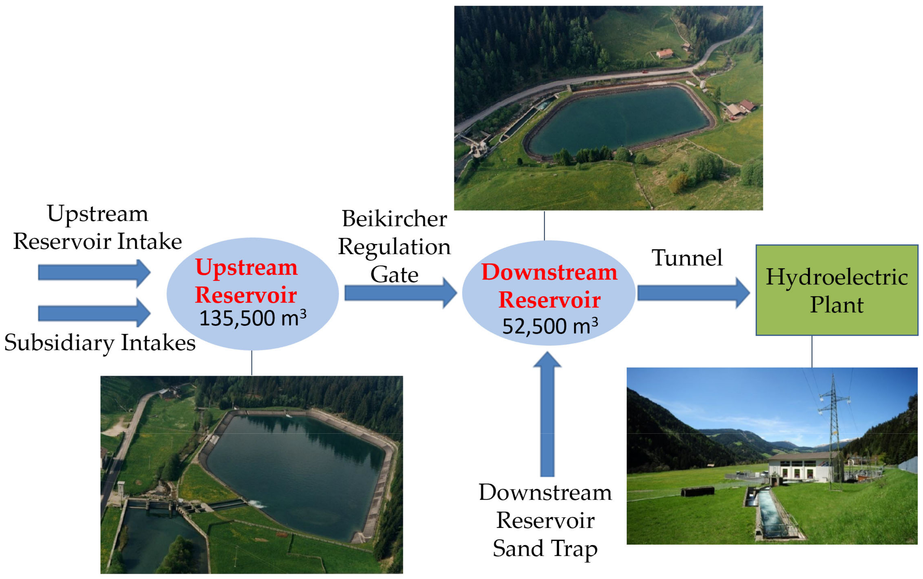
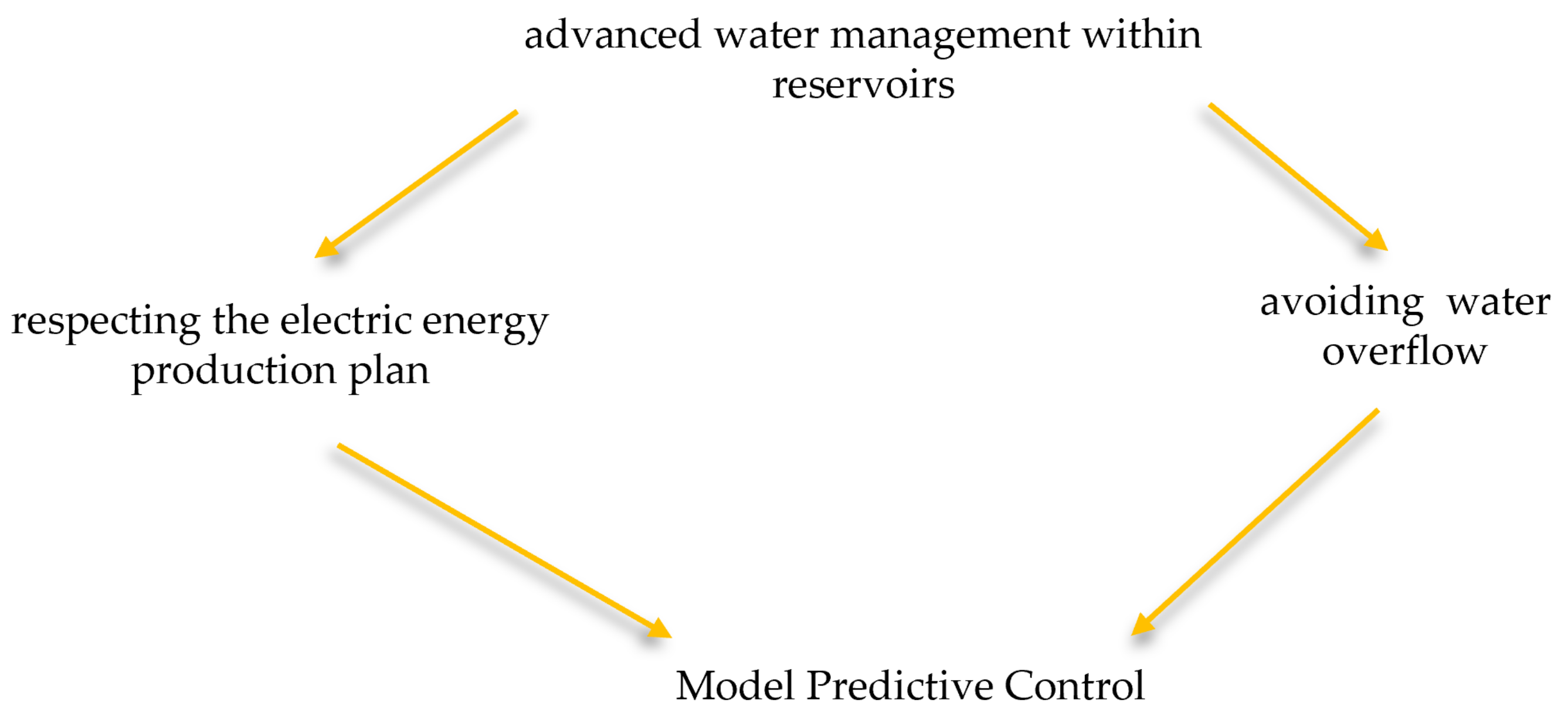
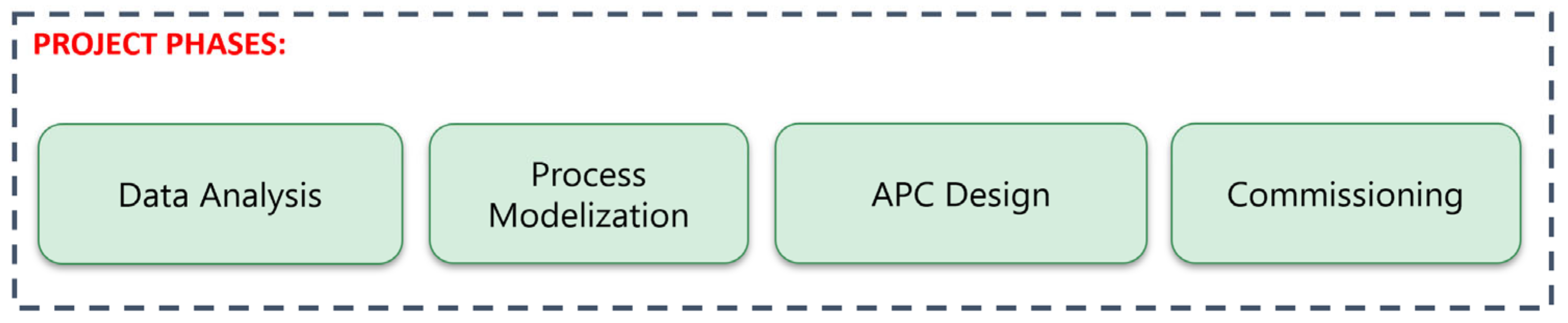
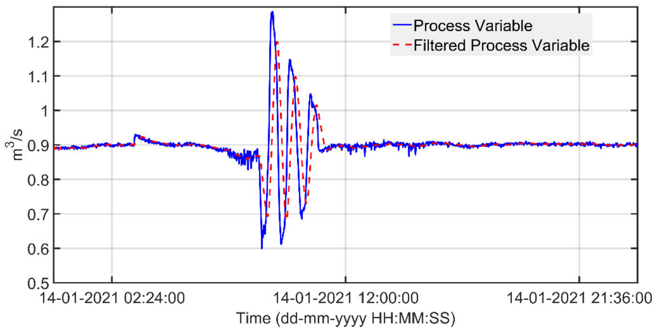
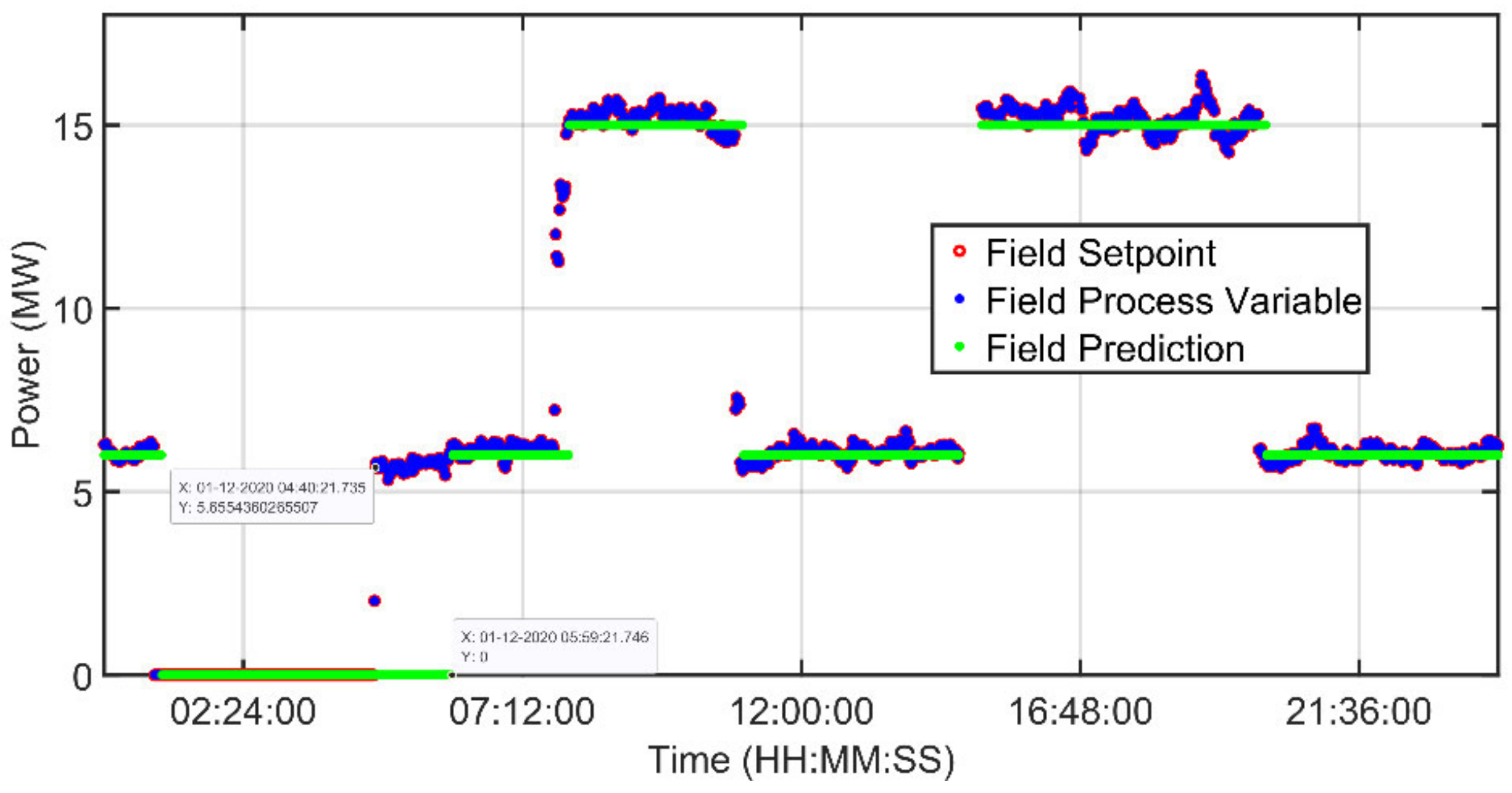
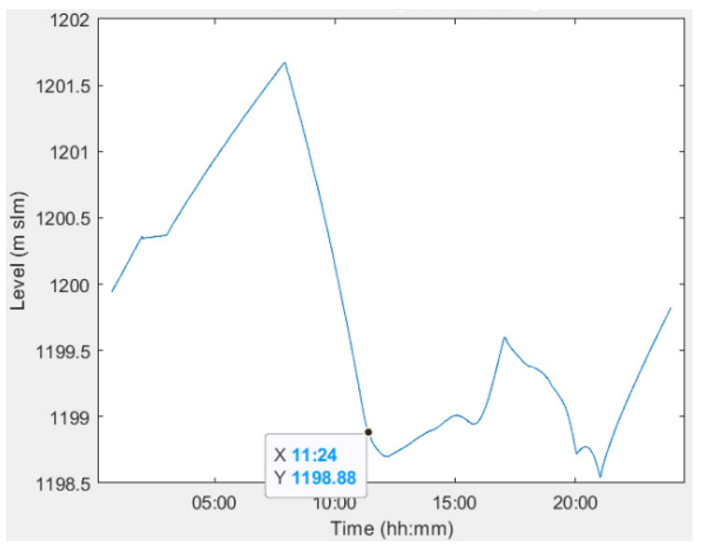
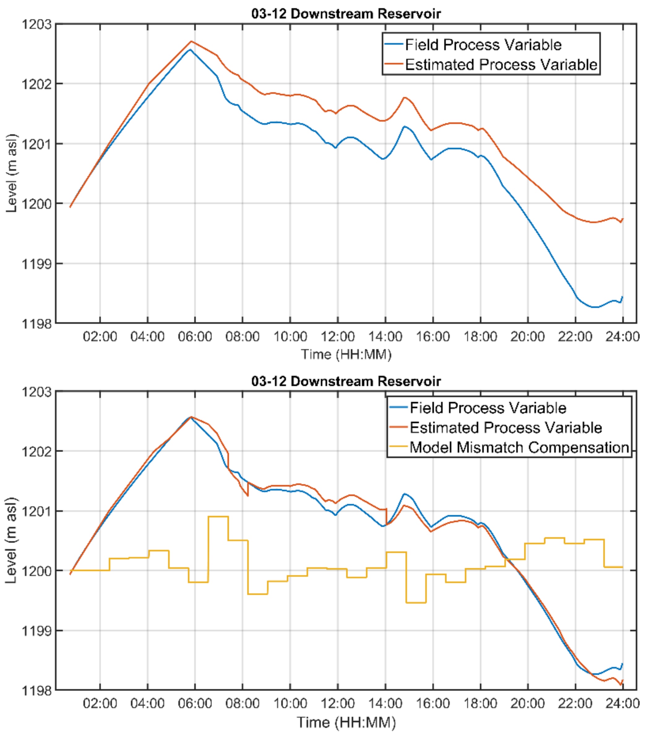
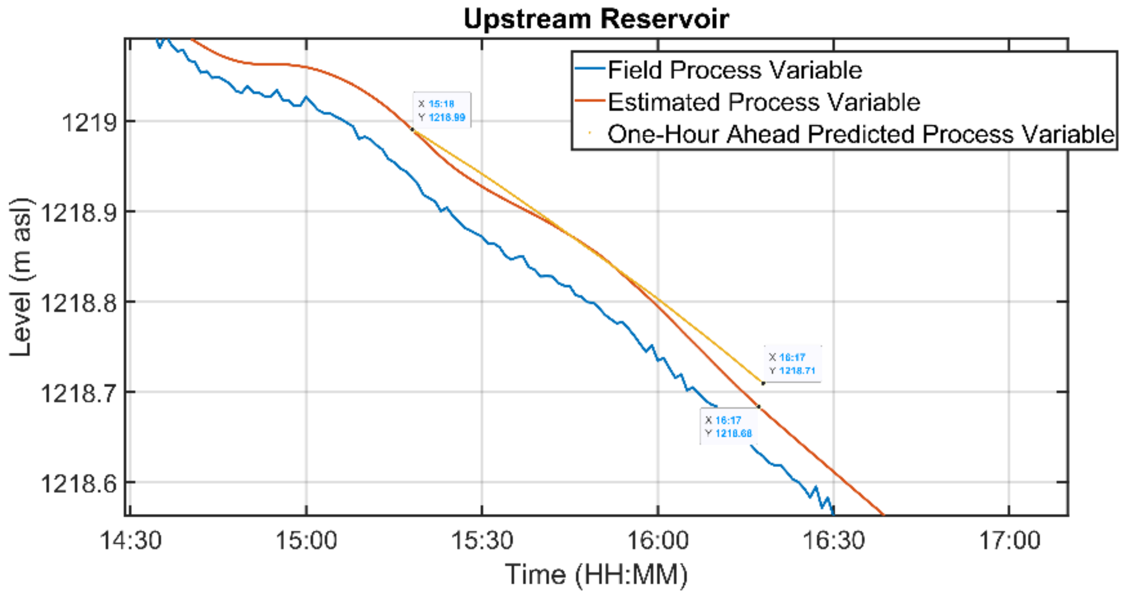
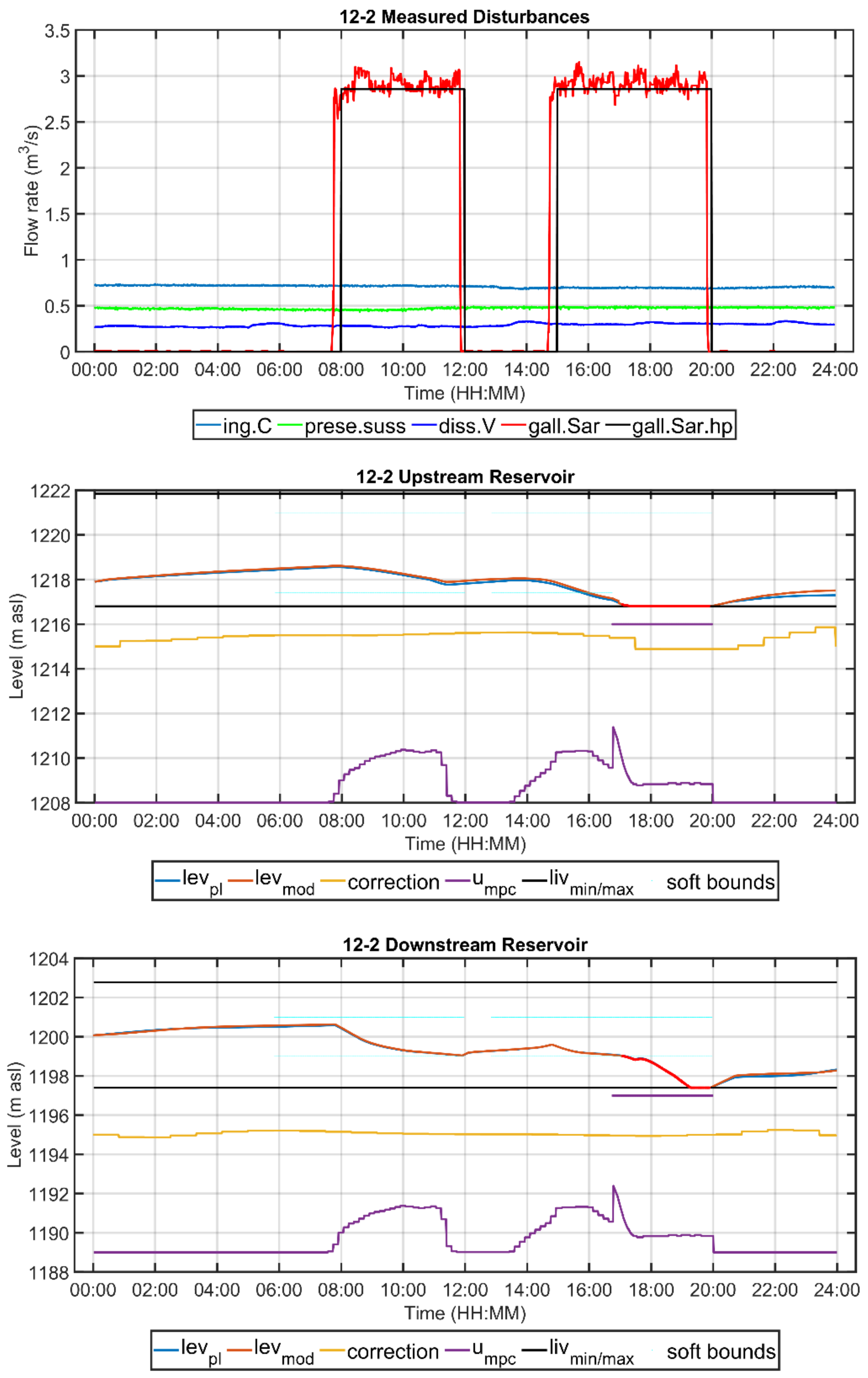
Table 1.
Parameters for the application of the Torricelli law to the regulation gate’s flow rate.
| Parameter | Value |
|---|---|
| 1.45 (m2) | |
| 9.81 (m/s2) | |
| (m) |
Disclaimer/Publisher’s Note: The statements, opinions and data contained in all publications are solely those of the individual author(s) and contributor(s) and not of MDPI and/or the editor(s). MDPI and/or the editor(s) disclaim responsibility for any injury to people or property resulting from any ideas, methods, instructions or products referred to in the content. |
© 2023 by the authors. Licensee MDPI, Basel, Switzerland. This article is an open access article distributed under the terms and conditions of the Creative Commons Attribution (CC BY) license (https://creativecommons.org/licenses/by/4.0/).
Share and Cite
MDPI and ACS Style
Zanoli, S.M.; Pepe, C.; Astolfi, G.; Luzi, F. Reservoir Advanced Process Control for Hydroelectric Power Production. Processes 2023, 11, 300. https://doi.org/10.3390/pr11020300
AMA Style
Zanoli SM, Pepe C, Astolfi G, Luzi F. Reservoir Advanced Process Control for Hydroelectric Power Production. Processes. 2023; 11(2):300. https://doi.org/10.3390/pr11020300
Chicago/Turabian StyleZanoli, Silvia Maria, Crescenzo Pepe, Giacomo Astolfi, and Francesco Luzi. 2023. "Reservoir Advanced Process Control for Hydroelectric Power Production" Processes 11, no. 2: 300. https://doi.org/10.3390/pr11020300
Note that from the first issue of 2016, this journal uses article numbers instead of page numbers. See further details here.