
Study on the Influencing Factors of the Response Characteristics of the Slide Valve-Type Direct-Acting Relief Valve with External Orifice
1
Department of Mechanical Design, School of Mechanical Engineering, Guizhou University, Guiyang 550025, China
2
Department of Water Resources and Hydropower Engineering, College of Civil Engineering, Guizhou University, Guiyang 550025, China
*
Author to whom correspondence should be addressed.
Processes 2023, 11(2), 397; https://doi.org/10.3390/pr11020397
Submission received: 23 December 2022
/
Revised: 21 January 2023
/
Accepted: 22 January 2023
/
Published: 28 January 2023
(This article belongs to the Special Issue Automation Control Systems & Process Control for Industry 4.0)
Abstract
:The slide valve-type direct-acting relief valve with external orifice (SVTDARVWEO) is widely used in hydraulic systems, and its response characteristics are influenced by key factors. It is of great significance to carry out research on the influencing factors of the response characteristics of the SVTDARVWEO. The working principle of the SVTDARVWEO is analyzed in the present study. The simulation model of the SVTDARVWEO is established using AMESim. The influence of the orifice diameter, viscosity coefficient, valve element mass, spring stiffness, oil seal length, and valve element diameter on the response characteristics of the SVTDARVWEO is studied. The results show that: (1) The smaller the orifice diameter is, the smaller the oscillation frequency, amplitude and maximum overshoot of pressure, flowrate, displacement and velocity are. (2) When the viscosity coefficient is 50 N/(m/s), 55 N/(m/s) and 60 N/(m/s), the pressure, flowrate, displacement and velocity oscillate periodically, but the amplitude of the oscillation decreases gradually, and the oscillation frequency is 250 Hz. When the viscosity coefficient is 60 N/(m/s), the pressure, flowrate, displacement and velocity will reach their respective stable values earlier. (3) When the valve element mass is 0.01 kg, 0.015 kg and 0.02 kg, the pressure, flowrate, displacement and velocity oscillate periodically, but the amplitude of oscillation decreases gradually. When the valve element mass is 0.01 kg, the pressure, flowrate, displacement and velocity will reach the stable value earlier. (4) The smaller the spring stiffness is, the greater the maximum overshoot of pressure, flowrate, displacement and velocity is, and the higher the number of oscillations to reach the stable value are, in addition to more time being required. (5) With the increase in oil seal length, the maximum overshoot of pressure and velocity, stability value of displacement also increase correspondingly. (6) With the increase in the valve element diameter, the stable value of pressure decreases, and the oscillation frequency of pressure, flowrate, displacement and velocity increase, but the oscillation amplitude decreases.
1. Introduction
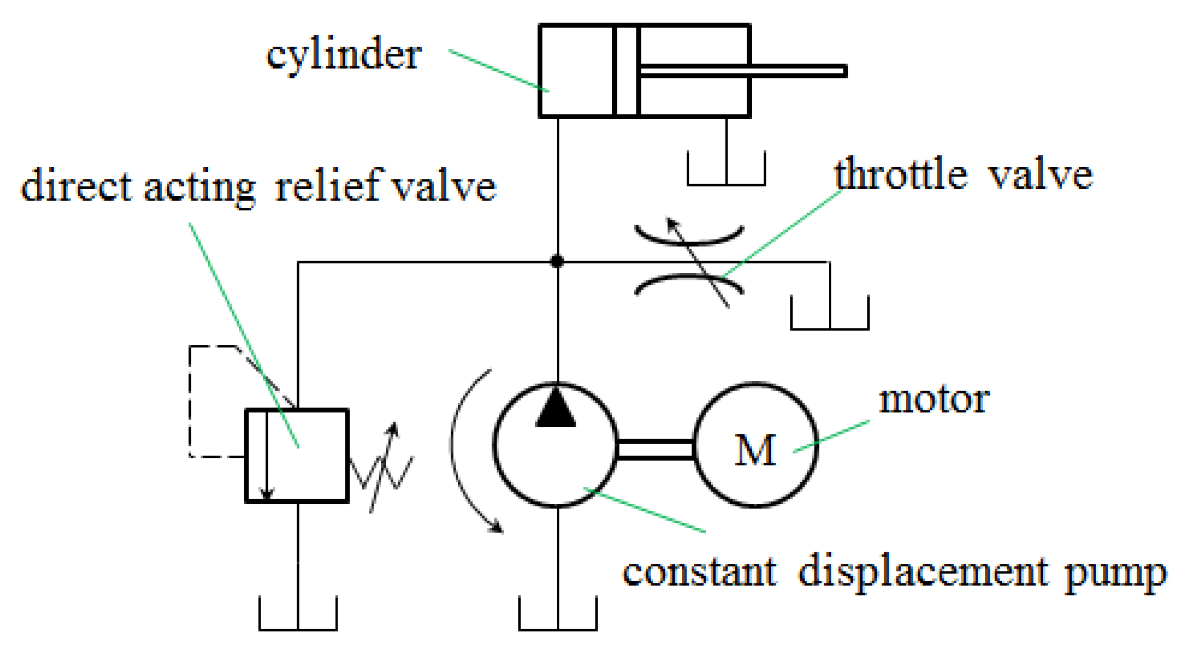
The direct-acting relief valve (DARV) relies on the pressure oil in the hydraulic system to directly act on the valve element to balance it with the spring force, so as to control the opening and closing of the overflow port in order to keep the hydraulic pressure of the controlled system or circuit constant, and to realize the functions of pressure stabilization, pressure regulation or pressure limitation. The application of the DARV mainly includes constant pressure overflow, safety protection, back-pressure generation, remote pressure regulation and multi-stage pressure control. (1) Constant pressure relief. Figure 1 is a typical inlet throttle speed-control system. When the system pressure is lower than the opening pressure of the DARV, the DARV will close. At this time, the system pressure depends on the load. When the system pressure reaches the set value of the DARV, the DARV is normally open and the system pressure is limited. When the load speed change of the actuator causes the flowrate change, the regulating function of the DARV keeps the system pressure essentially constant, and overflows the excess oil back to the tank, thus realizing constant pressure overflow. (2) Security protection. Figure 2 shows the parallel throttling speed-control circuit with a constant displacement pump. Figure 3 shows the volumetric throttling speed-control circuit with a variable displacement pump. Figure 4 shows the volumetric speed-control circuit with a variable/constant displacement pump/motor. In the above three circuits, the DARV is often used as a safety valve to prevent overloading of the system. Under normal conditions, the DARV is normally closed. When the system pressure is too high due to fault, abnormal load and other reasons, the DARV opens to overflow in order to protect the safety of the entire hydraulic system. (3) Back pressure generation. As shown in Figure 5, by connecting the DARV-3 to the oil return path of the actuator 4, a certain oil return resistance is created to improve the motion smoothness of the actuator. (4) Remote pressure regulation. As shown in Figure 6, by connecting the DARV-3 with the remote control port of the pilot relief valve and adjusting the pressure of the DARV-3, the pilot relief valve can be remotely regulated within the set pressure range. (5) Multi-stage pressure control. Figure 7 is a typical three-stage pressure control circuit. The DARV-2 and DARV-3 are connected with the remote control port of the pilot relief valve through a three-position four-way solenoid directional valve. The multi- stage pressure control of the hydraulic system is realized by switching the different working positions of the solenoid directional valve. The pressure regulating value of the pilot relief valve is set as p1, and the pressure regulating value of DARV-2 and DARV-3 are set as p2 and p3, respectively. When the solenoid directional valve works in the middle position, the working pressure of the system is p ≤ p1. When the solenoid directional valve is switched to the left and right positions, the working pressure of the system is p ≤ p2 and p ≤ p3, respectively.
The structure of the DARV mainly includes slide valve, cone valve, ball valve, etc. The SVTDARVWEO is widely used in medium- and low-pressure hydraulic systems due to its simple structure, easy processing, convenient adjustment and high sensitivity. However, the response characteristics of the SVTDARVWEO are influenced by factors such as the orifice’s diameter, viscosity coefficient, valve element mass, spring stiffness, oil seal length, and the valve element’s diameter. Therefore, it is of great significance to carry out research on the influencing factors of the response characteristics of the SVTDARVWEO.
In the last few decades, there have been many relevant studies on the direct-acting relief valve. Song et al. [1] developed a numerical model using CFD techniques to investigate the fluid and dynamic characteristics of a direct-operated safety relieve valve (SRV), and examined the comparison of the effects of the design parameters, including the adjusting ring position, vessel volume and spring stiffness. Burhani and Hos [2] addressed the static and dynamic behavior of a direct spring-operated PRV of conical shape in the presence of two-phase non-flashing flow, and recorded the effect of the system parameters, such as spring stiffness and reservoir capacity. Zong et al. [3] established the accuracy of CFD models for the prediction of the flow force exerted on the disk of a direct-operated pressure safety valve in energy system. Kadar et al. [4] presented a delayed oscillator model of pressure relief valves with outlet piping which contained a time delay originated in the pipe length and the velocity of sound in the pipe. Fu et al. [5] designed a direct-acting relief valve with permanent magnet spring to solve the problems of helical compression spring, and established the nonlinear model of air gap-magnetic force to reveal the impact of different configurations and air gap adjustments on magnetic field distribution. Burhani et al. [6] addressed the effect of non-flashing multiphase flow on the dynamic behavior of direct spring operated pressure relief valve, and developed a formula providing an order-of-magnitude estimation of the opening time of direct spring-operated pressure relief valve. Liao et al. [7] developed a two-degree-of-freedom fluid–structure coupling model of a direct-acting relief valve for underwater applications, and carried out parameter optimization with reliability analysis via an optimization closed loop. Zahariea [8] developed a functional diagram to perform numerical analysis of an electromagnetic normally closed direct-acting ball valve with cylindrical seat using the MATLAB/Simscape/SimHydraulics programming language. Wen et al. [9] developed a 2-DOF fluid–structure coupling dynamic model to explain the sudden jump of pressure as the variation of water depth for a direct-acting relief valve used by a torpedo pump as the variation of water depth. Erdodi and Hos [10] proposed two CFD-based methods for the analysis of the fluid forces and valve stability, including steady-state CFD method and dynamic CFD simulations. Liu et al. [11] established the mathematic model of sea water direct-acting relief valve (SDARV), and conducted related dynamic characteristic simulations. Wu et al. [12] established a mathematic model of a direct-operated seawater hydraulic relief valve under deep sea, and conducted stability analysis of the relief valve. Syrkin et al. [13] used the method of phase trajectories to establish the controller’s parameters and modes, and obtained the dynamic characteristics providing the absence of self-oscillations at the expense of additional damping of the shut-off and regulating elements. Raeder et al. [14] proposed an approach involving numerical simulation of non-stationary 3D gas dynamics, which enables one to determine a spatial structure of flow in a direct-acting safety valve and its quantitative characteristics (pressure, density, velocity, temperature). Sohn [15] investigated the fluid dynamics of a spring-loaded-type safety valve operated with steam through computational fluid dynamics (CFD), and analyzed the opening process by running the total ten-step simulations of lift level from 0 to 100%. Dempster et al. [16] questioned the accuracy of the scaling approach, examined the influence of the effect of built-up pressure in the discharge region of the safety relief valve, and investigated the problem theoretically using a CFD technique via the commercial code FLUENT. Zong et al. [17] performed the numerical and experimental investigation on a direct-operated pressure safety valve to deeply explore the mechanism of the discontinuities. Suzuki and Urata [18] developed a balanced-piston-type water hydraulic relief valve, which focused on preventing cavitation and improving the static characteristics and stability. Bazsó and Hős [19] presented some detailed experimental results on the static and dynamic behavior of a hydraulic pressure relief valve with a poppet valve body. Hős et al. [20] derived a model of an in-service direct-spring pressure relief valve, which coupled low-order rigid body mechanics for the valve to one-dimensional gas dynamics within the pipe. Hős, Bazsó and Champneys [21] developed a mathematical model of a spring-loaded pressure relief valve connected to a reservoir of compressible fluid via a single, straight pipe. Hős et al. [22] carried out the study of gas-service direct-spring pressure relief valves connected to a tank via a straight pipe by deriving a reduced-order model for predicting oscillatory instabilities such as valve flutter and chatter. Hyunjun, Dawon, and Sanghyun [23] used a multi-objective genetic algorithm to carry out the optimum design of direct spring-loaded pressure relief valve in water distribution system. Hyunjun et al. [24] explored the optimization of a direct spring-loaded pressure relief valve (DSLPRV) to consider the instability issue of a valve disk and the surge control for a pipeline system. Lei et al.’s [25] study concerned the flow model and dynamic characteristics of a direct spring-loaded poppet relief valve. Kim et al. [26] presented design concepts to improve the disadvantages of conventional direct-acting relief valves such as the low pressure precision, the low allowable flow rate, and unstable chattering phenomena. Dimitrov and Krstev [27] examined experimentally and theoretically the transients in hydraulic systems with direct-operated pressure relief valves, and determined the coefficient of hydrodynamic force acting on the valve poppet.
The novelty and significance of this work is that it establishes the AMESim simulation model of the SVTDARVWEO, and analyzes the influencing factors (such as the orifice’s diameter, viscosity coefficient, valve element mass, spring stiffness, oil seal length, and valve element diameter) of the response characteristics of the SVTDARVWEO systematically and comprehensively, provides theoretical basis for the design and manufacturing of the SVTDARVWEO, and offers a reference for the design and manufacturing of other valves, including pneumatic valves and hydraulic valves, helping manufacturers to reduce the development costs and shorten the development cycle.
The rest of this paper is organized as follows. In Section 2, the working principle of the SVTDARVWEO is analyzed. In Section 3, the AMESim simulation model of the SVTDARVWEO is established. The influence of the orifice’s diameter, viscosity coefficient, valve element mass, spring stiffness, oil seal length, valve element diameter on the response characteristics of the SVTDARVWEO is analyzed in Section 4. Finally, some conclusions are drawn in Section 5.
2. Working Principle of the SVTDARVWEO
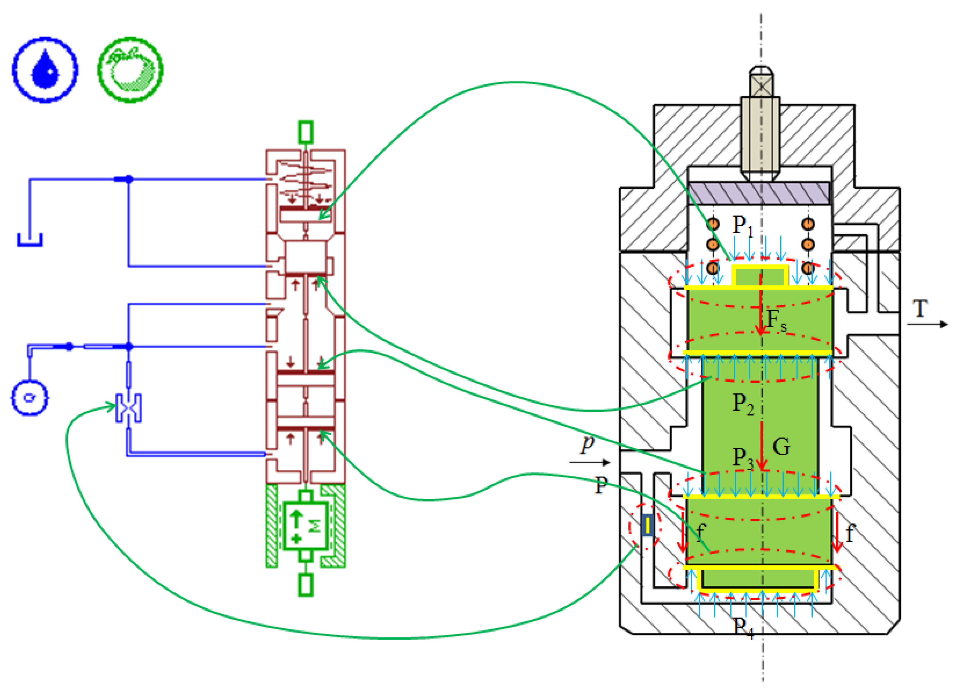
Figure 8 is the structural diagram of the SVTDARVWEO, the typical feature of which is that the orifice is not on the valve element but external to the valve element. The basic working principle of the SVTDARVWEO is as follows: the pressure oil of the hydraulic system flows to the inlet of the SVTDARVWEO (port ) through a pipe, and then it is divided into three paths: the first path acts on the ring with an area of at the upper part of the valve element (pressure: ); the second path acts on the ring with an area of at the lower part of the valve element (pressure: ); and the third path acts on the circular bottom with an area of at the lower part of the valve element (pressure: ) through thin pipes and orifice. In addition, the top of the valve element is affected by the pressure , and the effective area is . The valve element is jointly affected by the following forces: the hydraulic force () acting on the top of the valve element (area: ); the hydraulic force () acting on the upper part of the valve element (area: ); the hydraulic force () acting on the lower part of the valve element (area: ); the hydraulic force () acting on the bottom of the valve element (area: ); the mass force (); the spring force (); and the viscous friction force (). When the resultant force of the hydraulic forces acting on the valve element 3 is greater than the spring force, mass force, viscous friction occurs between the valve element and the valve body, and the valve port is opened, allowing the oil to overflow to the oil tank through the port T.
It can be seen from Figure 8 that , ; therefore, the values of and are equal and opposite, which can offset each other. In addition, since is connected to port , and . According to the above analysis, the resultant force of hydraulic forces acting on the valve element 3 is . As long as is satisfied, the valve port can be opened and the oil overflows to the oil tank.
3. AMESim Simulation Model of the SVTDARVWEO
With the development of fluid mechanics, hydraulic transmission, modern control theory, and other related disciplines in addition to the the rapid development of computer technology, hydraulic simulation technology and software are becoming an increasingly mature and become a powerful tool for designers of hydraulic components and systems. At present, hydraulic simulation software mainly includes MATLAB, EASY5, FluidSIM, HyPneu, DSHplus, HOPSAN, Automation Studio, 20-sim, AMESim, etc. Compared with other hydraulic simulation software, such as the familiar MATLAB, the biggest advantage of AMESim is that it does not need to establish the mathematical model of the system. The establishment, expansion or change of the simulation model is carried out through the graphical user interface, which frees users from numerical simulation algorithms, time-consuming programming, and tedious mathematical modeling, so as to focus on the design of the physical system itself in the engineering project, and modeling and simulation analysis can be conducted directly without special learning of programming language. Another advantage of AMESim is that it has a variety of simulation methods, such as batch-processing simulation, discontinuous continuous simulation, steady-state simulation, dynamic simulation, etc. It can dynamically switch the integration algorithm and adjust the integration step according to the characteristics of the system model at different simulation times, thus improving the stability of the system model and ensuring the accuracy of the simulation results.
AMESim is an advanced engineering system simulation modeling environment based on bond graph, integrating component libraries in mechanical, hydraulic, pneumatic, control, thermal, electrical and magnetic fields. Component libraries in different fields can be connected to each other, providing a complete platform for system engineering design, enabling users to build complex multidisciplinary simulation system models on the same platform and, on this basis, to conduct in-depth simulations and analysis, as well as to study the steady and dynamic performance of any component or system on this platform. HCD (hydraulic component design) is the library of hydraulic component designs in AMESim, which enables users to build sub models of any component from very basic modules, and to further study the steady and dynamic performance of the component, thus greatly enhancing the function of AMESim.
Based on the structure and working principle of the SVTDARVWEO, the AMESim simulation model of the valve is established using the hydraulic component design library (HCD), one-dimensional mechanical library (Mechanical), and standard hydraulic library (Hydraulic), as shown in Figure 9. In this model, the thick solid line represents the oil pressure action surface, and the arrow represents the pressure action’s direction. The four pressure action surfaces in the model correspond to the four pressure action surfaces of the valve element. The position of the orifice in the model corresponds to the position of the orifice in the structural diagram. The following basic assumptions were made when building the AMESim simulation model:
- (1)
- The operating temperature and ambient temperature do not change;
- (2)
- The physical and chemical properties of the working medium do not change;
- (3)
- The working medium is not polluted;
- (4)
- There is no geometric shape error between valve element and valve body;
- (5)
- The radial fit clearance between valve element and valve body is equal;
- (6)
- There is no assembly error between spring and valve element;
- (7)
- The foundation is stable without vibration;
- (8)
- The working environment is the earth, and the gravity acceleration remains unchanged, g = 9.8 m/s2;
- (9)
- No internal and external leakage;
- (10)
- The influence of gravity can be ignored;
- (11)
- All parts will not deform during operation.
4. Results and Discussion
Basic parameters: operating temperature °C, density , bulk modulus , absolute viscosity , flowrate . By changing the value of each parameter, the influence of each parameter on the response characteristics of the SVTDARVWEO is studied.
4.1. Influence of Orifice Diameter on Response Characteristics
The simulation parameters are shown in Table 1. The values of viscosity coefficient, valve element mass, spring stiffness, oil seal length, and valve element diameter remain constant, and the orifice’s diameter is set as 1 mm, 2 mm, 3 mm and 4 mm, respectively. The influence of the orifice’s diameter on the response characteristics of the SVTDARVWEO is studied.
The pressure response characteristics with orifice diameters of 1 mm~4 mm are shown in Figure 10a. The final stable value of the pressure is 10.02 bar. When the orifice diameters are 1 mm, 2 mm, 3 mm and 4 mm, the maximum pressure overshoot is about 4.608 bar, 2.712 bar, 2.353 bar and 2.26 bar, respectively. When the orifice’s diameter is 1 mm, the oscillation frequency is the lowest, about 167 Hz. When the orifice’s diameter is 2 mm, the oscillation frequency is about 200 Hz. When the orifice’s diameter is 3 mm and 4 mm, the oscillation frequency is close to about 250 Hz. In addition, when the orifice’s diameter is 1 mm, 2 mm, 3 mm and 4 mm, it needs to oscillate to about 0.06 s before the pressure can reach the stable value.
The flowrate response characteristics with an orifice’s diameter of 1 mm~4 mm are shown in Figure 10b. The final stable value of the flowrate is 10 L/min, and the flowrate before 0.004 s is 0 L/min. After 0.004 s, the flowrate oscillates to about 0.06 s before it becomes stable. When the orifice’s diameter is 1 mm, the oscillation frequency is the lowest, about 167 Hz. When the orifice’s diameter is 2 mm, the oscillation frequency is about 200 Hz. When the orifice’s diameter is 3 mm and 4 mm, the oscillation frequency is close to about 250 Hz. When the orifice’s diameter is 2 mm, the maximum flowrate overshoot is the highest, about 7.171 L/min. The maximum flowrate overshoot of orifice diameters of 1 mm, 3 mm and 4 mm is 6.646 L/min, 6.558 L/min and 6.37 1 L/min, respectively.
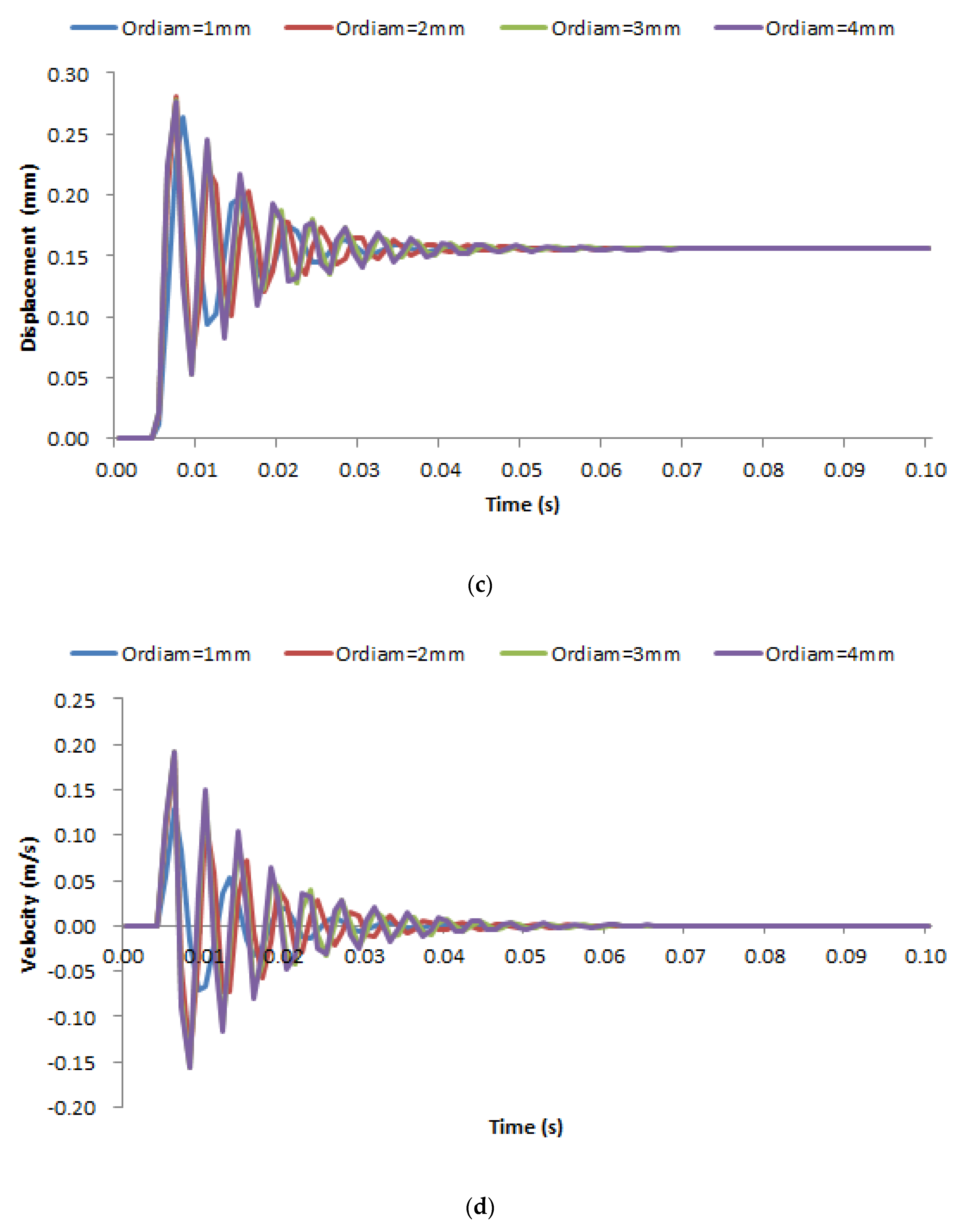
The displacement response characteristics of the valve with an orifice’s diameter of 1 mm~4 mm are shown in Figure 10c. The final stability value of the displacement is 0.156 mm, the displacement before 0.004 s is 0 mm, and the vibration after 0.004 s is about 0.06 s before it becomes stable. When the orifice’s diameter is 1 mm, the oscillation frequency is the lowest, about 167 Hz. When the orifice’s diameter is 2 mm, the oscillation frequency is about 200 Hz. When the orifice’s diameter is 3 mm and 4 mm, the oscillation frequency is close to about 250 Hz. When the orifice’s diameter is 1 mm, the maximum displacement overshoot is the lowest, about 0.107 mm. The maximum displacement overshoot of the orifice diameters of 2 mm, 3 mm and 4 mm is close, being 0.125 mm, 0.122 mm and 0.12 mm, respectively.
The velocity response characteristics of the valve element with an orifice’s diameter of 1 mm~4 mm are shown in Figure 10d. The final stable value of the valve element velocity is 0 m/s. The valve element velocity before 0.004 s is 0 m/s. After 0.004 s, the valve element velocity oscillates to about 0.06 s and is 0 m/s again. When the orifice’s diameter is 1 mm, the oscillation frequency is the lowest, about 167 Hz. When the orifice’s diameter is 2 mm, the oscillation frequency is about 200 Hz. When the orifice’s diameter is 3 mm and 4 mm, the oscillation frequency is close to about 250 Hz. When the orifice’s diameter is 1 mm, the peak velocity of the valve element is the lowest, about 0.13 m/s. The peak velocity of the valve element with orifice diameters of 2 mm, 3 mm and 4 mm is close, being 0.187 m/s, 0.192 m/s and 0.193 m/s, respectively.
4.2. Influence of Viscosity Coefficient on Response Characteristics
The simulation parameters are shown in Table 2. The values of orifice diameter, valve element mass, spring stiffness, oil seal length, valve element diameter remain constant, and the viscosity coefficient is set as 40 N/(m/s), 45 N/(m/s), 50 N/(m/s), 55 N/(m/s) and 60 N/(m/s), respectively. The influence of the viscosity coefficient on the response characteristics of the SVTDARVWEO is studied.
The pressure response characteristics with the viscosity coefficient of 40 N/(m/s)~60 N/(m/s) are shown in Figure 11a. When the viscosity coefficient is 40 N/(m/s) and 45 N/(m/s), the pressure oscillates periodically, the amplitude of the oscillation does not decrease, and the oscillation frequency is relatively high (333 Hz). When the viscosity coefficient is 50 N/(m/s), 55 N/(m/s) and 60 N/(m/s), the pressure oscillates periodically, but the amplitude of the oscillation gradually decreases, and the oscillation frequency is relatively low (250 Hz). In addition, it can be seen that the larger the viscosity coefficient is, the smaller the amplitude of pressure oscillation for adjacent oscillation periods is. It can be predicted that when the viscosity coefficient is 60 N/(m/s), the pressure will reach the stable value earlier.
The flowrate response characteristics with the viscosity coefficient of 40 N/(m/s)~60 N/(m/s) are shown in Figure 11b. The final stable value of flowrate is 10 L/min, and the flowrate before 0.004 s is 0 L/min. When the viscosity coefficient is 40 N/(m/s) and 45 N/(m/s), the flowrate oscillates periodically, the oscillation amplitude does not decrease, about 10 L/min, and the oscillation frequency is relatively high (333 Hz). When the viscosity coefficient is 50 N/(m/s), 55 N/(m/s) and 60 N/(m/s), the flowrate oscillates periodically, but the amplitude of the oscillation gradually decreases, and the oscillation frequency is relatively low (250 Hz). In addition, it can be seen that the larger the viscosity coefficient is, the smaller the amplitude of flowrate oscillation for adjacent oscillation periods is. It can be predicted that when the viscosity coefficient is 60 N/(m/s), the flowrate will reach the stable value earlier.
The displacement response characteristics of the valve element with the viscosity coefficient of 40 N/(m/s)~60 N/(m/s) are shown in Figure 11c. The displacement before 0.004 s is 0 mm. When the viscosity coefficient is 40 N/(m/s) and 45 N/(m/s), the displacement oscillates periodically, the amplitude of the oscillation does not decrease (about 0.165 mm), and the oscillation frequency is relatively high (333 Hz). When the viscosity coefficient is 50 N/(m/s), 55 N/(m/s) and 60 N/(m/s), the displacement oscillates periodically, but the amplitude of the oscillation gradually decreases, and the oscillation frequency is relatively low (250 Hz). In addition, it can be seen that the larger the viscosity coefficient is, the smaller the amplitude of displacement oscillation for adjacent oscillation periods is. It can be predicted that when the viscosity coefficient is 60 N/(m/s), the displacement will reach the stable value earlier.
The velocity response characteristics of the valve element with the viscosity coefficient of 40 N/(m/s)~60 N/(m/s) are shown in Figure 11d. The velocity before 0.004 s is 0 m/s. When the viscosity coefficient is 40 N/(m/s) and 45 N/(m/s), the velocity oscillates periodically, the amplitude of the oscillation does not decrease (about 0.3 m/s), and the oscillation frequency is relatively high (333 Hz). When the viscosity coefficient is 50 N/(m/s), 55 N/(m/s) and 60 N/(m/s), the velocity oscillates periodically, but the amplitude of the oscillation gradually decreases, and the oscillation frequency is relatively low (250 Hz). In addition, it can be seen that the larger the viscosity coefficient is, the smaller the amplitude of velocity oscillation for adjacent oscillation periods is. It can be predicted that when the viscosity coefficient is 60 N/(m/s), the velocity will reach the stable value earlier.
4.3. Influence of Valve Element Mass on Response Characteristics
The simulation parameters are shown in Table 3. The values of orifice diameter, viscosity coefficient, spring stiffness, oil seal length, and valve element diameter remain constant. The valve element mass are set to 0.01 kg, 0.015 kg, 0.025 kg, 0.025 kg and 0.03 kg, respectively. The influence of the valve element mass on the response characteristics of the SVTDARVWEO is studied.
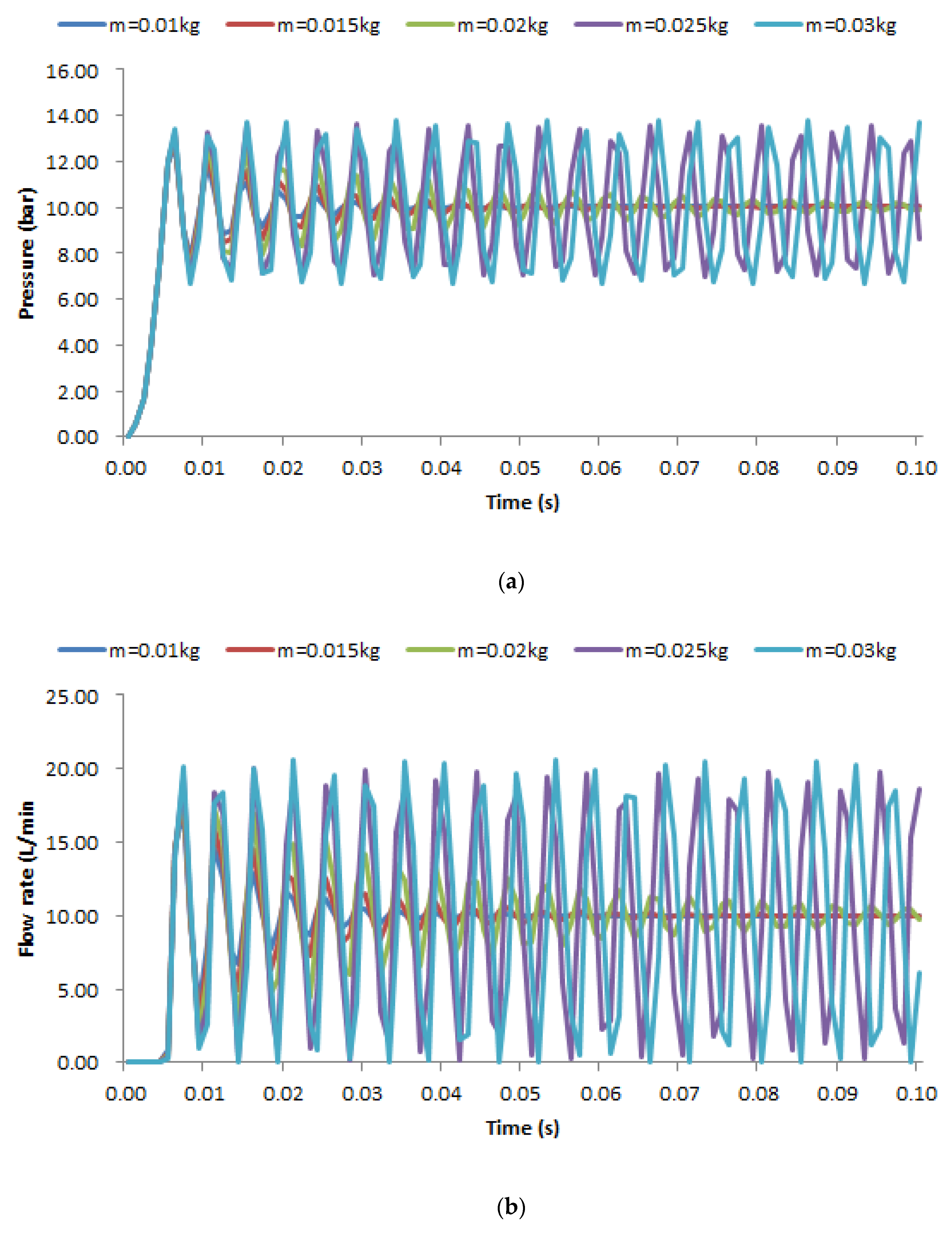
The pressure response characteristics of a valve element with a mass of 0.01 kg~0.03 kg are shown in Figure 12a. When the valve element mass is 0.025 kg and 0.03 kg, the pressure oscillates periodically and the amplitude of the oscillation does not decrease (about 3.5 bar). When the valve element mass is 0.01 kg, 0.015 kg and 0.02 kg, the pressure oscillates periodically but the amplitude of oscillation decreases gradually. In addition, it can be seen that the pressure oscillation frequency is about 200 Hz. With the increase in valve element mass, the pressure oscillation frequency will decrease, but not to a large extent. The smaller the valve element mass is, the smaller the amplitude of pressure oscillation for adjacent oscillation periods is. It can be predicted that when the valve element mass is 0.01 kg, the pressure will reach the stable value earlier.
The flowrate response characteristics of a valve element with a mass of 0.01 kg~0.03 kg are shown in Figure 12b. The final stable value of flowrate is 10 L/min, and the flowrate before 0.004 s is 0 L/min. When the valve element mass is 0.025 kg and 0.03 kg, the flowrate rate oscillates periodically and the oscillation amplitude does not decrease (about 10 L/min). When the valve element mass is 0.01 kg, 0.015 kg and 0.02 kg, the flowrate rate oscillates periodically, but the amplitude of oscillation decreases gradually. In addition, it can be seen that the oscillation frequency is about 200 Hz. As the valve element mass increases, the flowrate oscillation frequency will decrease, but the reduction is not significant. The smaller the valve element mass is, the smaller the amplitude of flowrate oscillation for adjacent oscillation periods is. It can be predicted that when the valve element mass is 0.01 kg, the flowrate will reach the stable value earlier.
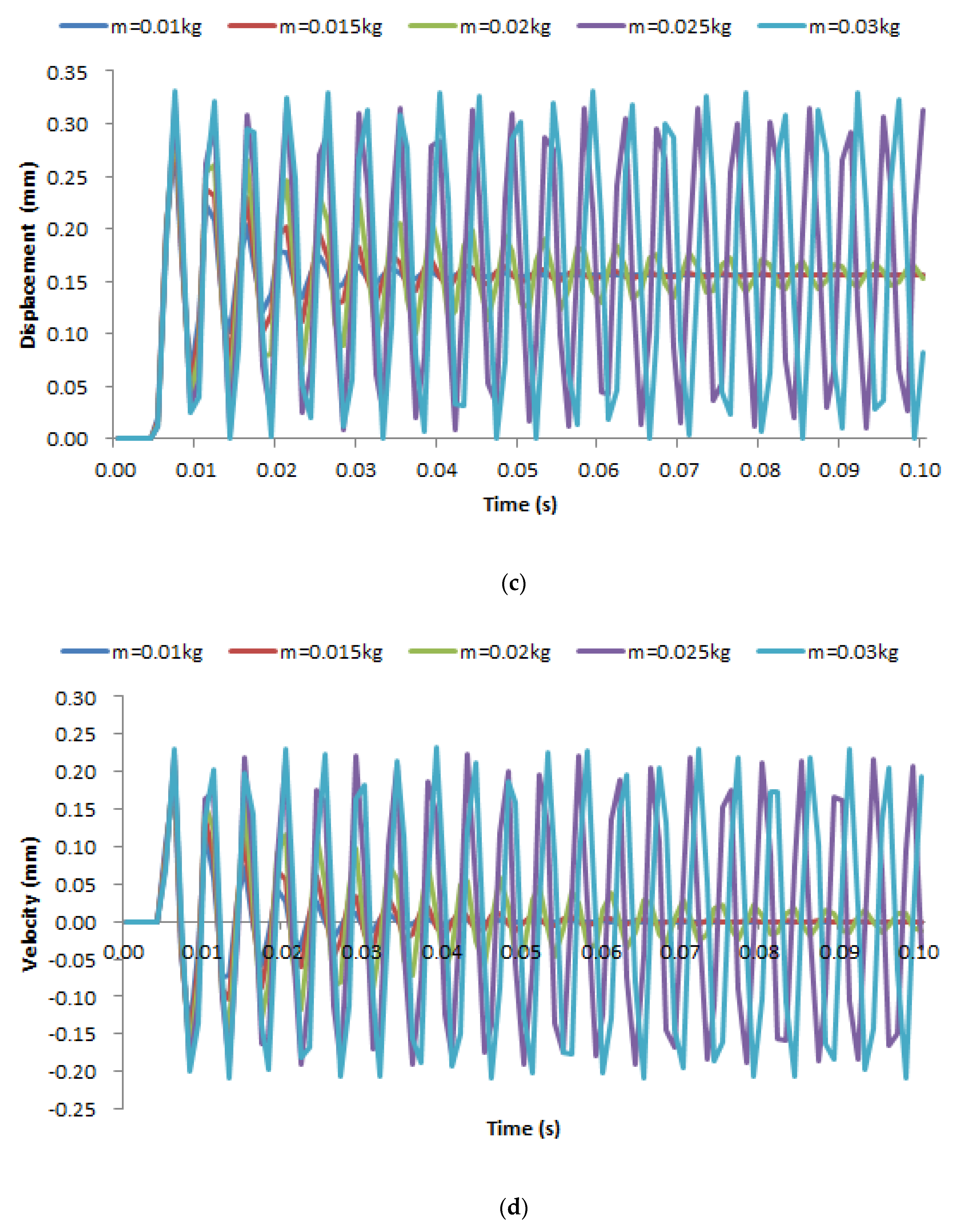
The displacement response characteristics of a valve element with a mass of 0.01 kg~0.03 kg are shown in Figure 12c. The displacement before 0.004 s is 0 mm. When the valve element mass is 0.025 kg and 0.03 kg, the displacement oscillates periodically and the oscillation amplitude does not decrease, which is about 0.170 mm. When the valve element mass is 0.01 kg, 0.015 kg and 0.02 kg, the displacement oscillates periodically but the amplitude of the oscillation decreases gradually. In addition, it can be seen that the oscillation frequency is about 200 Hz. With the increase in the valve element mass, the displacement oscillation frequency will decrease, but not to a large extent. The smaller the valve element mass is, the smaller the amplitude of displacement oscillation for adjacent oscillation periods is. It can be predicted that when the valve element mass is 0.01 kg, the displacement will reach the stable value earlier.
The velocity response characteristics of a valve element with a mass of 0.01 kg~0.03 kg are shown in Figure 12d. The velocity before 0.004 s is 0 m/s. When the valve element mass is 0.025 kg and 0.03 kg, the velocity oscillates periodically and the amplitude of oscillation does not decrease, which is about 0.25 m/s. When the valve element mass is 0.01 kg, 0.015 kg and 0.02 kg, the velocity oscillates periodically but the amplitude of the oscillation decreases gradually. In addition, it can be seen that the oscillation frequency is about 200 Hz. With the increase in the valve element mass, the velocity oscillation frequency will decrease, but to a small extent. The smaller the valve element mass is, the smaller the amplitude of velocity oscillation for adjacent oscillation periods is. It can be predicted that when the valve element mass is 0.01 kg, the velocity will reach the stable value earlier.
4.4. Influence of Spring Stiffness on Response Characteristics
The simulation parameters are shown in Table 4. The values of orifice diameter, viscosity coefficient, valve element mass, oil seal length, and valve element diameter remain constant, and the spring stiffness is set to 1 N/mm, 10 N/mm, 20 N/mm, 30 N/mm, 50 N/mm, respectively. The influence of spring stiffness on the response characteristics of the SVTDARVWEO is studied.
The pressure response characteristics with a spring stiffness of 1 N/mm~50 N/mm are shown in Figure 13a. The pressure corresponding to different values of spring stiffness oscillates and the oscillation frequency is about 250 Hz. After a certain oscillation, the pressure will eventually reach the stable value. The corresponding pressure stability values for a spring stiffness of 1 N/mm, 10 N/mm, 20 N/mm, 30 N/mm and 50 N/mm are 10.020 bar, 10.197 bar, 10.390 bar, 10.580 bar and 10.950 bar, respectively, and the corresponding maximum pressure overshoots are 2.712 bar, 2.613 bar, 2.504 bar, 2.396 bar and 2.184 bar, respectively. When the spring stiffness is 1 N/mm, the number of oscillations to reach the stable pressure value is the largest and the time required is the longest, but the opening pressure is the lowest. When the spring stiffness is 50 N/mm, the number of oscillations to reach the stable pressure value is the lowest and the time required is the shortest, but the opening pressure is the highest.
The flowrate response characteristics with a spring stiffness of 1 N/mm~50 N/mm are shown in Figure 13b. The flowrate before 0.004 s is 0 L/min, and 0.007 s reaches the maximum flowrate overshoot. The flowrate corresponding to different spring stiffness values oscillates and the oscillation frequency is about 250 Hz. After a certain oscillation, the flowrate will eventually reach the stable value of 10 L/min. The greater the spring stiffness is, the smaller the maximum flowrate overshoot is. The maximum flowrate overshoot corresponding to a spring stiffness of 1 N/mm, 10 N/mm, 20 N/mm, 30 N/mm and 50 N/mm is 7.171 L/min, 6.679 L/min, 6.168 L/min, 5.692 L/min and 4.84 L/min, respectively. When the spring stiffness is 1 N/mm, the number of oscillations is the maximum and the time to reach the stable flowrate value is the longest. When the spring stiffness is 50 N/mm, the number of oscillations to reach the stable flowrate value is the lowest and the time required is the shortest.
The displacement response characteristics with a spring stiffness of 1 N/mm~50 N/mm are shown in Figure 13c. The displacement before 0.004 s is 0 mm, and the maximum displacement overshoot is reached at 0.007 s. The displacement corresponding to different spring stiffness values oscillates and the oscillation frequency is about 250 Hz. After a certain oscillation, the displacement will eventually reach the stable value. The displacement stability values corresponding to a spring stiffness of 1 N/mm, 10 N/mm, 20 N/mm, 30 N/mm and 50 N/mm are 0.156 mm, 0.155 mm, 0.153 mm, 0.152 mm and 0.149 mm, respectively, and the corresponding maximum displacement overshoots are 0.125 mm, 0.114 mm, 0.103 mm, 0.093 mm and 0.076 mm, respectively. When the spring stiffness is 1 N/mm, the number of oscillations is the maximum and the time to reach the stable displacement value is the longest. When the spring stiffness is 50 N/mm, the number of oscillations to reach the stable displacement value is the lowest and the time required is the shortest.
The velocity response characteristics with spring stiffness of 1 N/mm~50 N/mm are shown in Figure 13d. The velocity before 0.004 s is 0 m/s, and the maximum velocity overshoot is reached at 0.006 s. The velocity corresponding to different spring stiffness values oscillates and the oscillation frequency is about 250 Hz. After a certain oscillation, the velocity will eventually reach the stable value of 0 m/s. The maximum velocity overshoots corresponding to spring stiffness of 1 N/mm, 10 N/mm, 20 N/mm, 30 N/mm and 50 N/mm are 0.187 m/s, 0.178 m/s, 0.169 m/s, 0.16 m/s and 0.144 m/s, respectively. When the spring stiffness is 1 N/mm, the number of oscillations is the maximum and the time to reach the stable velocity value is the longest. When the spring stiffness is 50 N/mm, the number of oscillations to reach the stable velocity value is the lowest and the time required is the shortest.
4.5. Influence of Oil Sealing Length on Response Characteristics
The simulation parameters are shown in Table 5. The values of orifice diameter, viscosity coefficient, valve element mass, spring stiffness, and valve element diameter remain constant. The oil sealing length is set as 0 mm, 0.5 mm, 1.0 mm, 1.5 mm and 2.0 mm respectively. The influence of oil sealing length on the response characteristics of the SVTDARVWEO is studied.
The pressure response characteristics of the SVTDARVWEO with an oil seal length of 0 mm~2 mm are shown in Figure 14a. The pressure corresponding to different oil sealing lengths oscillates with a frequency of about 200 Hz. After a certain oscillation, the pressure finally reaches the stable value of 10.02 bar. With the increase in oil seal length, the time to reach the maximum pressure overshoot increases correspondingly, and the maximum pressure overshoot also increases correspondingly. The maximum pressure overshoot corresponding to the sealing length of 0 mm, 0.5 mm, 1.0 mm, 1.5 mm and 2.0 mm is 2.712 bar, 7.625 bar, 10.214 bar, 13.707 bar and 13.683 bar, respectively.
The flowrate response characteristics of the SVTDARVWEO with an oil seal length of 0 mm~2 mm are shown in Figure 14b. The flowrate corresponding to different seal oil lengths oscillates with the oscillation frequency of about 200 Hz. After a certain oscillation, the flowrate finally reaches the stable value of 10 L/min. With the increase in oil sealing length, the time for overflow port to generate flowrate and the time for reaching the maximum flowrate overshoot increase accordingly. The maximum flowrate overshoot corresponding to the oil seal length of 0 mm, 0.5 mm, 1.0 mm, 1.5 mm and 2.0 mm is 7.171 L/min, 17.002 L/min, 24.806 L/min, 33.488 L/min and 25.167 L/min, respectively. It is worth noting that the maximum flowrate overshoot does not occur when the maximum oil seal length is 2 mm, but when the oil seal length is 1.5 mm.
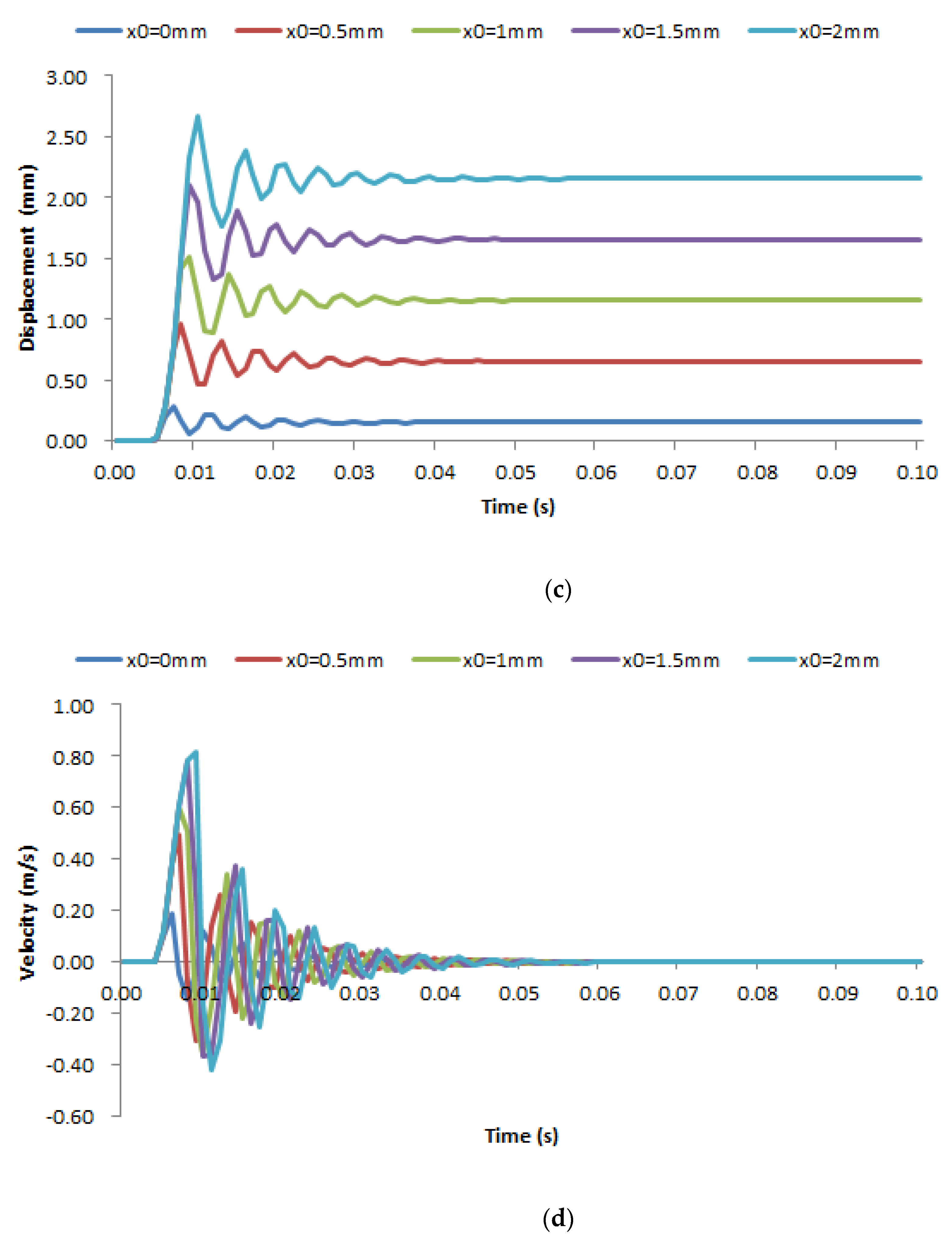
The displacement response characteristics of the SVTDARVWEO with an oil seal length of 0 mm~2 mm are shown in Figure 14c. The displacement corresponding to different oil sealing lengths has oscillation, and the oscillation frequency is about 200 Hz. After a certain oscillation, the displacement finally reaches its own displacement stability value. With the increase in oil seal length, the displacement stability value and the time to reach the displacement stability value also increase correspondingly. The displacement stability values corresponding to the sealing length of 0 mm, 0.5 mm, 1.0 mm, 1.5 mm and 2.0 mm are 0.156 mm, 0.656 mm, 1.156 mm, 1.656 mm and 2.156 mm, respectively. With the increase in oil sealing length, the maximum overshoot of displacement increases correspondingly. The maximum overshoot of displacement corresponding to the oil sealing lengths of 0 mm, 0.5 mm, 1.0 mm, 1.5 mm and 2.0 mm is 0.125 mm, 0.313 mm, 0.362 mm, 0.449 mm and 0.516 mm, respectively.
The velocity response characteristics of the SVTDARVWEO with an oil seal length of 0 mm~2 mm are shown in Figure 14d. The velocity corresponding to oil seal lengths oscillates, with an oscillation frequency of about 200 Hz. With the increase in oil seal length, the time to reach the velocity stability value increases correspondingly, and the maximum overshoot of velocity increases correspondingly. The maximum overshoot of velocity corresponding to an oil seal length of 0 mm, 0.5 mm, 1.0 mm, 1.5 mm, and 2.0 mm is 0.187 m/s, 0.493 m/s, 0.602 m/s, 0.78 m/s, and 0.813 m/s, respectively.
4.6. Influence of Valve Element Diameter on Response Characteristics
The simulation parameters are shown in Table 6. The values of orifice diameter, viscosity coefficient, valve element mass, spring stiffness, and oil seal length remain constant. The valve element diameters are set as 10 mm, 11 mm, 12 mm, 13 mm, 14 mm and 15 mm, respectively. The influence of valve element diameter on the response characteristics of the SVTDARVWEO is studied.
The pressure response characteristics of a valve element with a diameter of 10 mm~15 mm are shown in Figure 15a. The pressure corresponding to different valve element diameters oscillates, and the pressure finally reaches its stable value after a certain oscillation. With the increase in valve element diameter, the pressure stability value decreases. The pressure stability values corresponding to the valve element diameters of 10 mm, 11 mm, 12 mm, 13 mm, 14 mm and 15 mm are 10.02 bar, 10.015 bar, 10.011 bar, 10.009 bar, 10.007 bar and 10.006 bar, respectively. In addition, it is easy to see that with the increase in valve element diameter, the pressure oscillation frequency increases and the pressure oscillation amplitude decreases.
The flowrate response characteristics of a valve element with a diameter of 10 mm~15 mm are shown in Figure 15b. The flowrate before 0.004 s is 0 L/min, and the flowrate corresponding to different valve element diameters oscillates. After a certain oscillation, the flowrate finally reaches the stable value of 10 L/min. With the increase in valve element diameter, the flowrate oscillation frequency increases and the flowrate oscillation amplitude decreases.
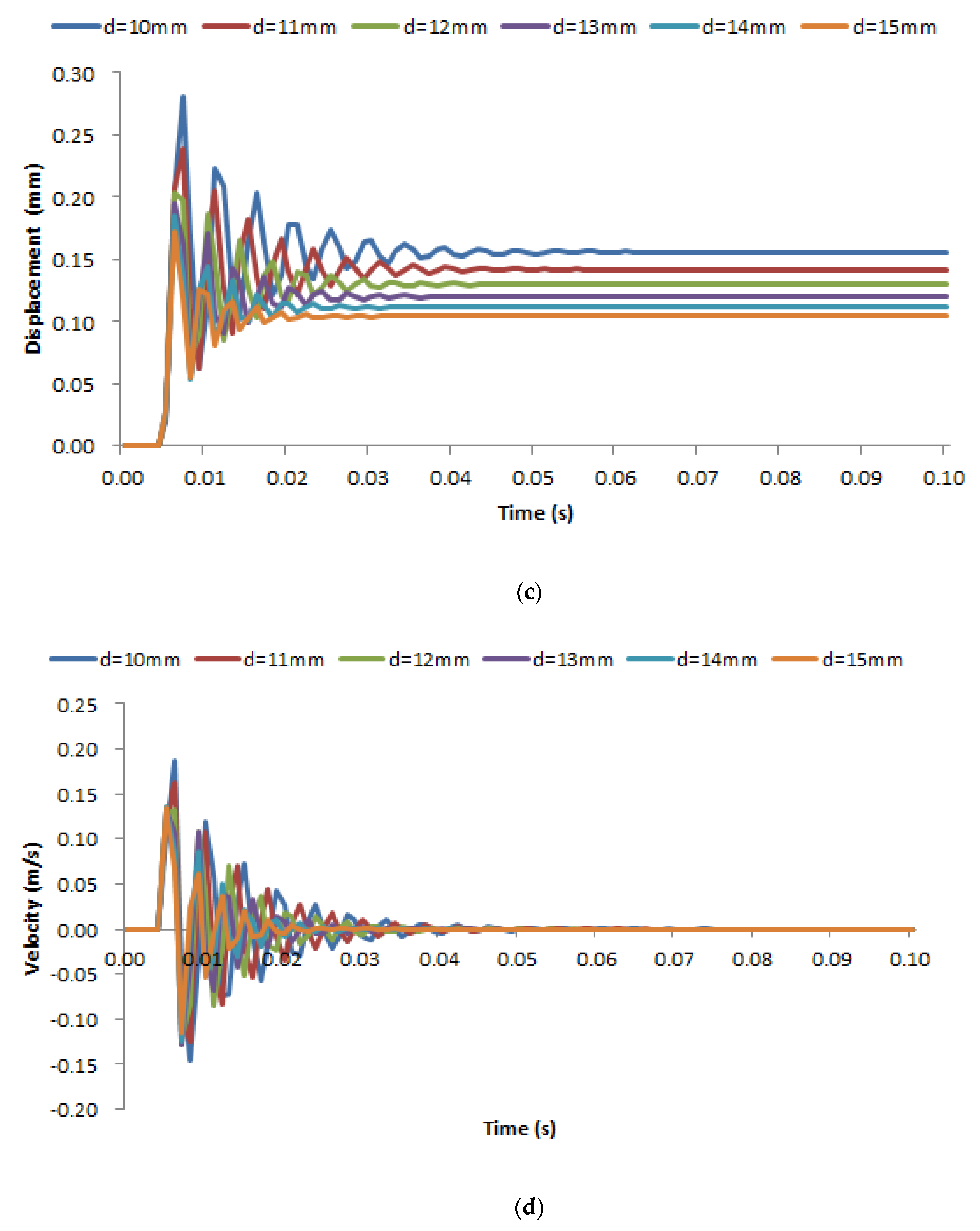
The displacement response characteristics of a valve element with a diameter of 10 mm~15 mm are shown in Figure 15c. The displacement before 0.004 s is 0 mm, and the displacement corresponding to different valve element diameters oscillates. After a certain oscillation, the displacement finally reaches its respective stable value. As the valve element diameter increases, the displacement stability value decreases. The displacement stability values corresponding to the valve element diameters of 10 mm, 11 mm, 12 mm, 13 mm, 14 mm and 15 mm are 0.156 mm, 0.142 mm, 0.130 mm, 0.120 mm, 0.112 mm and 0.104 mm, respectively. With the increase in the valve element diameter, the displacement oscillation frequency increases while the amplitude decreases, and the time for the displacement to reach the stable value also decreases.
The velocity response characteristics of a valve element with a diameter of 10 mm~15 mm are shown in Figure 15d. The velocity before 0.004 s is 0 m/s. The velocity corresponding to different valve element diameters oscillates. After a certain oscillation, the velocity finally reaches the stable value of 0 m/s. With the increase in valve element diameter, the frequency of velocity oscillation increases while the amplitude of oscillation decreases, and the time for the velocity to reach the stable value also decreases.
5. Conclusions
Based on the working principle of the SVTDARVWEO, the simulation model of the SVTDARVWEO is established using AMESim. The influence of orifice diameter, viscosity coefficient, valve element mass, spring stiffness, oil seal length, and valve element diameter on the response characteristics of the SVTDARVWEO is analyzed, and the following conclusions are obtained:
- (1)
- The smaller the orifice diameter is, the smaller the oscillation frequency, amplitude and maximum overshoot of pressure, flowrate, displacement, and velocity is. When the orifice diameter is 1 mm, the oscillation frequency is the lowest, about 167 Hz. When the orifice diameter is 2 mm, the oscillation frequency is about 200 Hz. When the orifice diameter is 3 mm and 4 mm, the oscillation frequency is close to about 250 Hz. The flowrate, displacement and velocity before 0.004 s are 0, and the pressure, flowrate, displacement and velocity will oscillate to about 0.06 s to reach individual stable values.
- (2)
- When the viscosity coefficient is 40 N/(m/s) and 45 N/(m/s), the pressure, flowrate, displacement and velocity oscillate periodically, the amplitude of the oscillation does not decrease, and the oscillation frequency is about 333 Hz. When the viscosity coefficient is 50 N/(m/s), 55 N/(m/s) and 60 N/(m/s), the pressure, flowrate, displacement and velocity oscillate periodically, but the amplitude of the oscillation gradually decreases, and the oscillation frequency is about 250 Hz. The flowrate, displacement and velocity before 0.004 s are 0. When the viscosity coefficient is 60 N/(m/s), the pressure, flowrate, displacement and velocity will reach individual stable values earlier.
- (3)
- When the valve element mass is 0.025 kg and 0.03 kg, the pressure, flowrate, displacement and velocity oscillate periodically and the amplitude of oscillation does not decrease. When the valve element mass is 0.01 kg, 0.015 kg and 0.02 kg, the pressure, flowrate, displacement and velocity oscillate periodically, but the amplitude of oscillation decreases gradually. The oscillation frequency is about 200 Hz. As the valve element mass increases, the displacement oscillation frequency will decrease, but to a small extent. The flowrate, displacement and velocity before 0.004 s are 0. When the valve element mass is 0.01 kg, the pressure, flowrate, displacement and velocity will reach individual stable values earlier.
- (4)
- When the spring stiffness is 1 N/mm~50 N/mm, the pressure, flowrate, displacement and velocity corresponding to different spring stiffness values oscillate and the oscillation frequency is about 250 Hz. After the oscillation, the pressure, flowrate, displacement and velocity will eventually reach individual stable values. The greater the spring stiffness is, the smaller the maximum overshoot of pressure, flowrate, displacement and velocity is. The flowrate, displacement and velocity before 0.004 s are 0. When the spring stiffness is 1 N/mm, the pressure, flowrate, displacement and velocity return to individual stable values with the largest number of oscillations and the longest time required. When the spring stiffness is 50 N/mm, the number of oscillations of pressure, flowrate, displacement and velocity to reach individual stable values is the lowest and the time required is the shortest.
- (5)
- The pressure, flowrate, displacement and velocity corresponding to different oil seal lengths will oscillate, and the oscillation frequency is about 200 Hz. After certain oscillations, the pressure, flowrate, displacement and velocity finally reach individual stable values. With the increase in oil sealing length, the time to reach the maximum overshoot of pressure, the maximum overshoot of pressure, the time to generate flow at the overflow port, and the time to reach the maximum overshoot of flow all increase correspondingly. At the same time, the displacement stability value and the time to reach the displacement stability value increase correspondingly, with the time to reach the velocity stability value and the maximum overshoot of velocity increasing correspondingly.
- (6)
- When the valve element diameter is 10 mm~15 mm, the pressure corresponding to different valve element diameters oscillate, and the pressure, flowrate, displacement and velocity will finally reach individual stable values after certain oscillations. The flowrate, displacement and velocity before 0.004 s are 0. With the increase in valve element diameter, the stable value of pressure decreases, the oscillation frequency of pressure, flowrate, displacement and velocity increases, the oscillation amplitude decreases, and the time for displacement and velocity to reach individual stable values also decreases.
Author Contributions
Conceptualization, H.L.; methodology, H.L.; validation, Q.Z.; formal analysis, Q.Z.; investigation, Q.Z.; data curation, H.L.; writing—original draft preparation, H.L.; writing—review and editing, Q.Z.; supervision, Q.Z.; funding acquisition, H.L. All authors have read and agreed to the published version of the manuscript.
Funding
This research received no external funding.
Data Availability Statement
The data presented in this study are available on request from the corresponding author.
Acknowledgments
This work is supported by the National Natural Science Foundation of China [grant number 51365008], and the Joint Foundation of Science and Technology Department of Guizhou Province [grant number Qiankehe LH Zi [2015]7658]. The authors are grateful to them for their support.
Conflicts of Interest
The authors declare no conflict of interest.
References
- Song, X.; Cui, L.; Cao, M.; Cao, W.; Park, Y.; Dempster, W.M. A CFD analysis of the dynamics of a direct-operated safety relief valve mounted on a pressure vessel. Energy Convers. Manag. 2014, 81, 407–419. [Google Scholar] [CrossRef] [Green Version]
- Burhani, M.G.; Hős, C. An Experimental and Numerical Analysis on the Dynamical Behavior of a Safety Valve in the Case of Two-phase Non-flashing Flow. Period. Polytech.-Chem. Eng. 2021, 65, 251–260. [Google Scholar] [CrossRef]
- Zong, C.Y.; Zheng, F.; Chen, D.; Dempster, W.; Song, X. Computational Fluid Dynamics Analysis of the Flow Force Exerted on the Disk of a Direct-Operated Pressure Safety Valve in Energy System. J. Press. Vessel. Technol.-Trans. Asme 2020, 142, 011702. [Google Scholar] [CrossRef]
- Kadar, F.; Hos, C.; Stepan, G. Delayed oscillator model of pressure relief valves with outlet piping. J. Sound Vib. 2022, 534, 117016. [Google Scholar] [CrossRef]
- Fu, C.Y.; Yang, L.; Si, G.; Li, Y. Design and Mechanical Performance Analysis of Relief Valve with Permanent Magnet Spring. In Proceedings of the IEEE/CSAA International Conference on Aircraft Utility Systems (AUS), Beijing, China, 10–12 October 2016. [Google Scholar]
- Burhani, M.G.; Hős, C. Estimating the opening time of a direct spring operated pressure relief valve in the case of multiphase flow of fixed mass fraction in the absence of piping. J. Loss Prev. Process Ind. 2020, 66, 104169. [Google Scholar] [CrossRef]
- Liao, M.L.; Zheng, Y.; Gao, Z.; Song, W. Fluid-structure coupling modelling and parameter optimization of a direct-acting relief valve for underwater application. Nonlinear Dyn. 2021, 105, 2935–2958. [Google Scholar] [CrossRef]
- Zahariea, D. Functional Diagram for Modeling the Electromagnetic Ball Valve with Cylindrical Seat. In Proceedings of the Innovative Manufacturing Engineering Conference (IManE), Chisinau, Moldova, 29–30 May 2014. [Google Scholar]
- Song, W.; Yang, C.; Zhang, X.; Li, Y. Mathematical Modelling and Dynamic Analysis of a Direct-Acting Relief Valve Based on Fluid-Structure Coupling Analysis. Shock. Vib. 2021, 2021, 5581684. [Google Scholar] [CrossRef]
- Erdődi, I.; Hős, C. Prediction of quarter-wave instability in direct spring operated pressure relief valves with upstream piping by means of CFD and reduced order modelling. J. Fluids Struct. 2017, 73, 37–52. [Google Scholar] [CrossRef]
- Liu, Y.S.; Ren, X.; Wu, D.; Li, D.; Li, X. Simulation and analysis of a seawater hydraulic relief valve in deep-sea environment. Ocean. Eng. 2016, 125, 182–190. [Google Scholar]
- Wu, S.; Li, C.; Deng, Y. Stability Analysis of a Direct-Operated Seawater Hydraulic Relief Valve under Deep Sea. Math. Probl. Eng. 2017, 2017, 5676317. [Google Scholar] [CrossRef] [Green Version]
- Syrkin, V.V.; Balakin, P.D.; Treyer, V.A. Study on hydraulic direct-acting relief valve. J. Phys. Conf. Ser. 2017, 858, 12035. [Google Scholar] [CrossRef]
- Raeder, T.; Tenenev, V.; Chernova, A.; Koroleva, M. Multilevel Simulation of Direct Operated Safety Valve. In Proceedings of the Ivannikov Ispras Open Conference (ISPRAS), Moscow, Russia, 22–23 November 2018. [Google Scholar]
- Sohn, S. A Numerical Analysis of Direct Spring Loaded Type—Steam Safety Valve Using CFD Simulation. In Proceedings of the 22nd International Conference Nuclear Energy for New Europe (NENE), Bled, Slovenia, 9–12 September 2013. [Google Scholar]
- Dempster, W.; Taggart, S.; Doyle, C. Limitations in the Use of Pressure Scaling for Safety Relief Valve Design. In Proceedings of the ASME Pressure Vessels and Piping Conference (PVP 2018), Prague, Czech Republic, 15–20 July 2018. [Google Scholar]
- Zong, C.Y.; Zheng, F.J.; Song, X.G. Understanding Lift Force Discontinuity of Pressure Safety Valve. In Proceedings of the ASME Pressure Vessels and Piping Conference, San Antonio, TX, USA, 14–19 July 2019. [Google Scholar]
- Suzuki, K.; Urata, E. Development of a Direct Pressure-Sensing Water Hydraulic Relief Valve. Int. J. Fluid Power 2008, 9, 5–13. [Google Scholar] [CrossRef]
- Bazsó, C.; Hős, C.J. An experimental study on the stability of a direct spring loaded poppet relief valve. J. Fluids Struct. 2013, 42, 456–465. [Google Scholar] [CrossRef]
- Hős, C.J.; Champneys, A.; Paul, K.; McNeely, M. Dynamic behavior of direct spring loaded pressure relief valves in gas service: Model development, measurements and instability mechanisms. J. Loss Prev. Process Ind. 2014, 31, 70–81. [Google Scholar] [CrossRef] [Green Version]
- Hős, C.; Bazsó, C.; Champneys, A. Model reduction of a direct spring-loaded pressure relief valve with upstream pipe. IMA J. Appl. Math. 2015, 80, 1009–1024. [Google Scholar] [CrossRef] [Green Version]
- Hős, C.J.; Champneys, A.; Paul, K.; McNeely, M. Dynamic behaviour of direct spring loaded pressure relief valves in gas service: II reduced order modelling. J. Loss Prev. Process Ind. 2015, 36, 1–12. [Google Scholar] [CrossRef] [Green Version]
- Kim, H.; Baek, D.; Kim, S. Optimum design of direct spring loaded pressure relief valve in water distribution system using multi-objective genetic algorithm. J. Korean Soc. Water Wastewater 2018, 32, 115–122. [Google Scholar] [CrossRef]
- Kim, H.; Kim, S.; Kim, Y.; Kim, J. Optimization of Operation Parameters for Direct Spring Loaded Pressure Relief Valve in a Pipeline System. J. Press. Vessel. Technol. 2018, 140, 051603. [Google Scholar] [CrossRef]
- Lei, J.; Tao, J.; Liu, C.; Wu, Y. Flow model and dynamic characteristics of a direct spring loaded poppet relief valve. Proc. Inst. Mech. Eng. Part C J. Mech. Eng. Sci. 2017, 232, 1657–1664. [Google Scholar] [CrossRef]
- Kim, S.D.; Kim, J.H. Conceptual Design on a Direct-Operated Relief Valve with High-Precision and Large-Flow. Proceedings of the Academic Conference of the Active Pressure Construction Machinery Society. 2021, 52. Available online: https://www.dbpia.co.kr/Journal/articleDetail?nodeId=NODE10755358 (accessed on 1 December 2022).
- Dimitrov, S.; Krstev, D. Modelling and Simulation of the Transient Performance of a Direct Operated Pressure Relief Valve. Hidraulica 2022, 3, 75–81. [Google Scholar]
Figure 1.
Constant pressure relief circuit of inlet throttle speed-control system.

Figure 2.
The parallel throttling speed-control circuit with constant displacement pump.

Figure 3.
The volumetric throttling speed-control circuit with variable displacement pump.
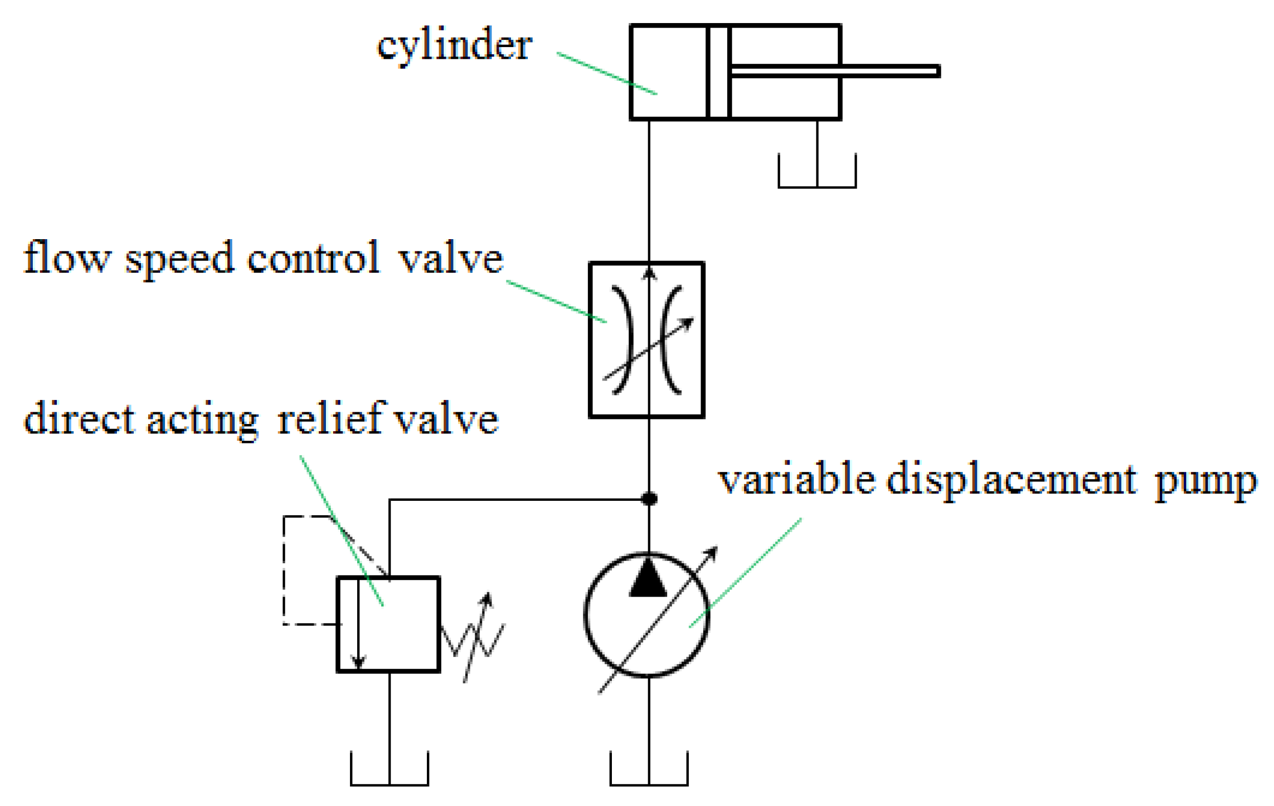
Figure 4.
The volumetric speed-control circuit with variable/constant displacement pump/motor. (a) VDP—CDM, (b) CDP—VDM, (c) VDP—VDM.
Figure 4.
The volumetric speed-control circuit with variable/constant displacement pump/motor. (a) VDP—CDM, (b) CDP—VDM, (c) VDP—VDM.
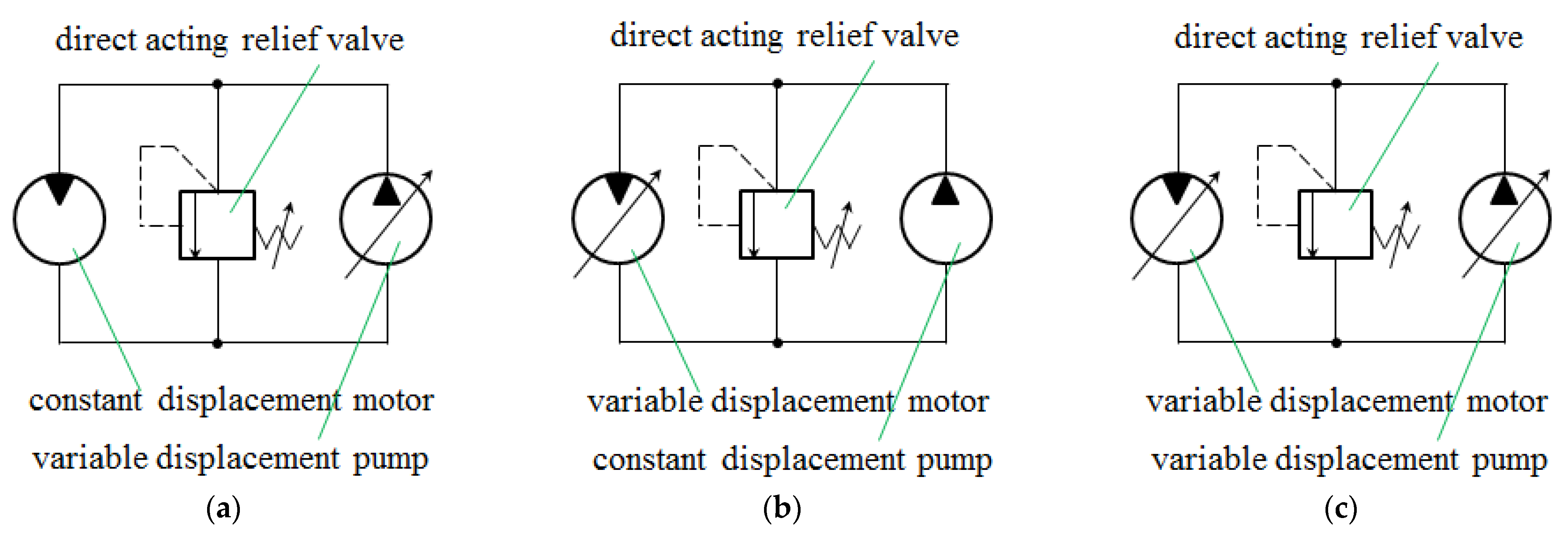
Figure 5.
The back pressure generation circuit.
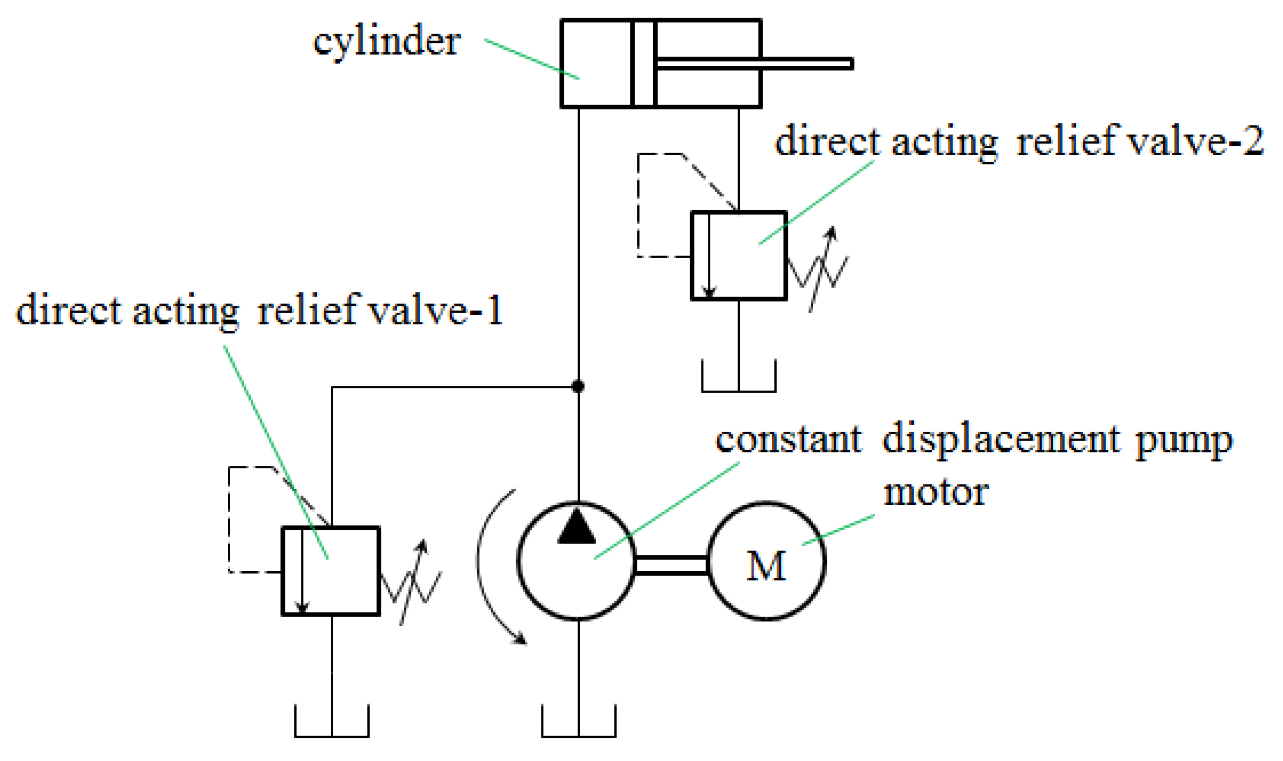
Figure 6.
The remote pressure regulation circuit.
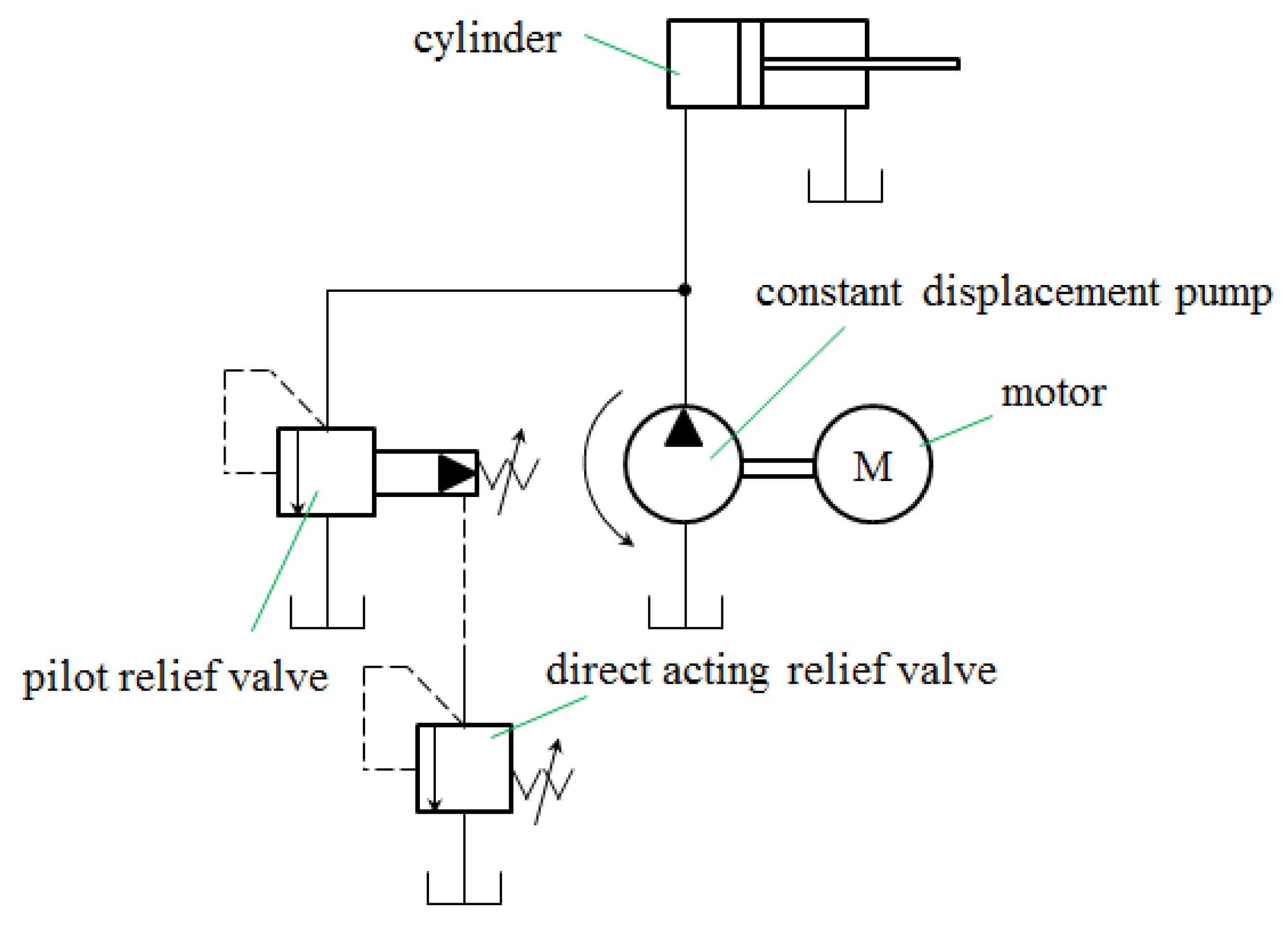
Figure 7.
The multi-stage pressure control circuit.
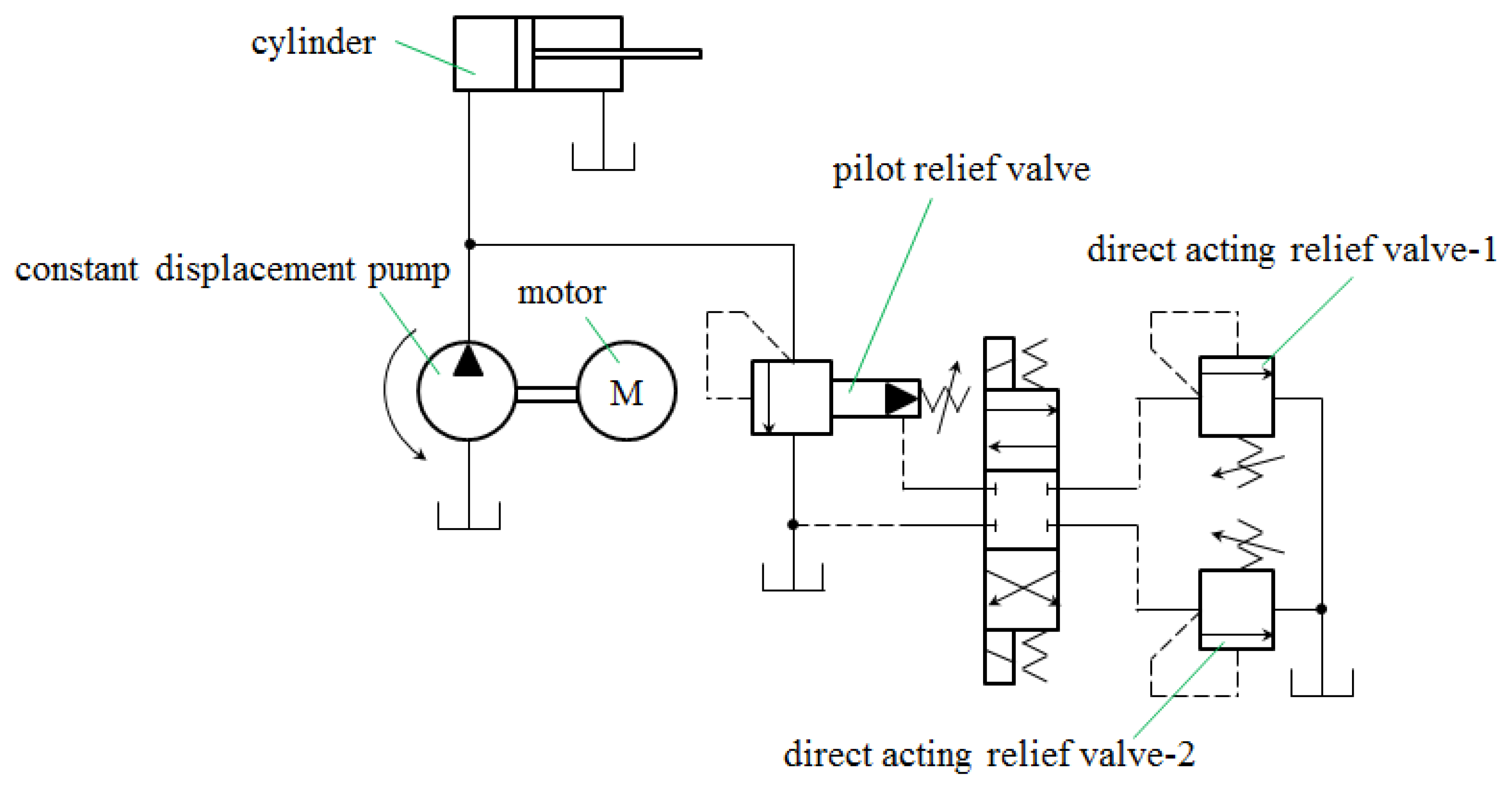
Figure 8.
The structural diagram of the SVTDARVWEO.

Figure 9.
AMESim simulation model of the SVTDARVWEO.

Figure 10.
(a) The pressure response characteristics—orifice diameter: 1 mm~4 mm. (b) The flowrate response characteristics—orifice diameter: 1 mm~4 mm. (c) The displacement response characteristics of the valve element—orifice diameter: 1 mm~4 mm. (d) The velocity response characteristics of the valve element—orifice diameter: 1 mm~4 mm.


Figure 11.
(a) The pressure response characteristics—viscosity coefficient: 40~60 N/(m/s). (b) The flowrate response characteristics—viscosity coefficient: 40~60 N/(m/s). (c) The displacement response characteristics of the valve element—viscosity coefficient: 40~60 N/(m/s). (d) The velocity response characteristics of the valve element—viscosity coefficient: 40~60 N/(m/s).

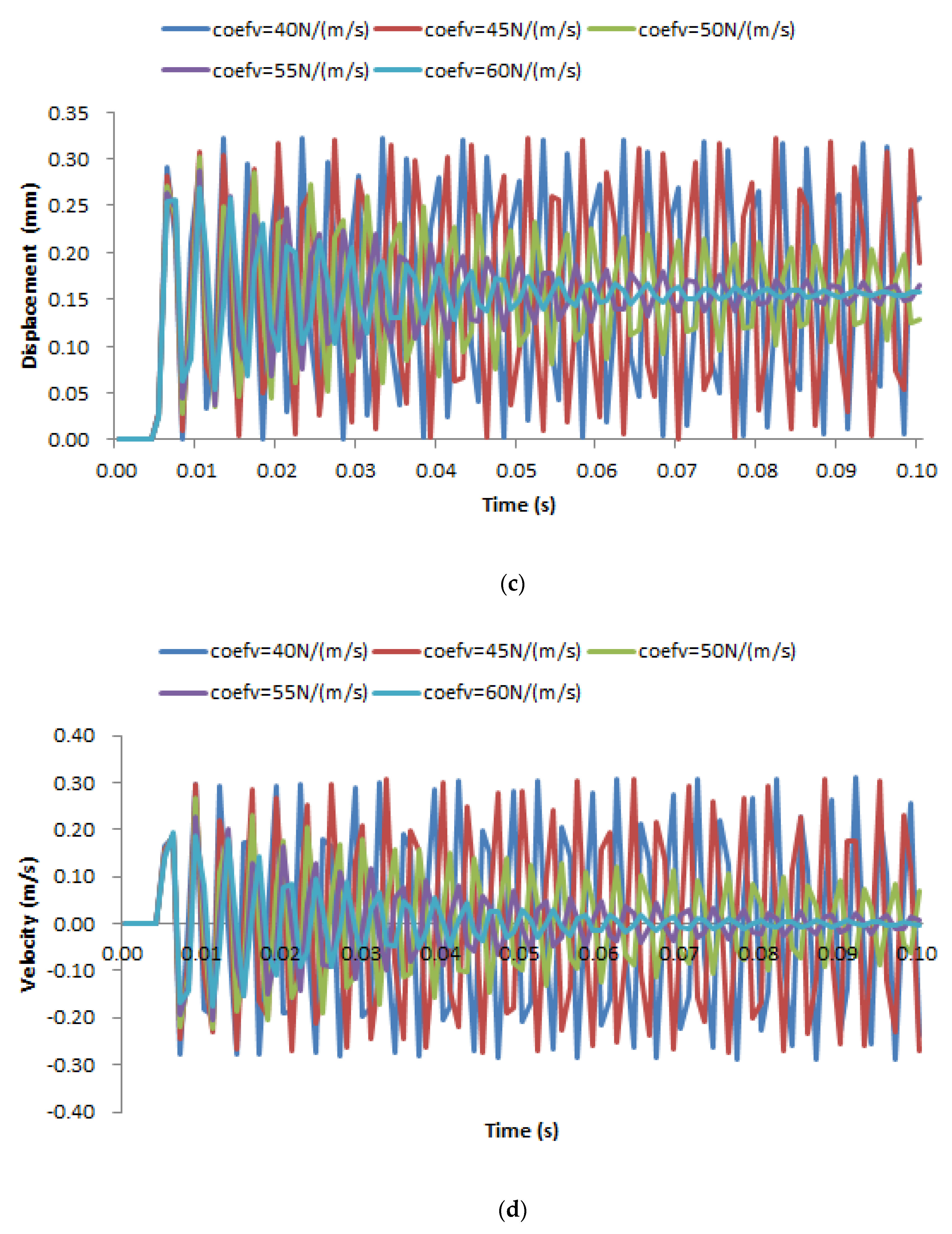
Figure 12.
(a) The pressure response characteristics—valve element mass: 0.01~0.03 kg. (b) The flowrate response characteristics—valve element mass: 0.01~0.03 kg. (c) The displacement response characteristics—valve element mass: 0.01~0.03 kg. (d) The velocity response characteristics—valve element mass: 0.01~0.03 kg.


Figure 13.
(a) The pressure response characteristics—spring stiffness: 1~50 N/mm. (b) The flowrate response characteristics—spring stiffness: 1~50 N/mm. (c) The displacement response characteristics—spring stiffness: 1~50 N/mm. (d) The velocity response characteristics—spring stiffness: 1~50 N/mm.
Figure 13.
(a) The pressure response characteristics—spring stiffness: 1~50 N/mm. (b) The flowrate response characteristics—spring stiffness: 1~50 N/mm. (c) The displacement response characteristics—spring stiffness: 1~50 N/mm. (d) The velocity response characteristics—spring stiffness: 1~50 N/mm.

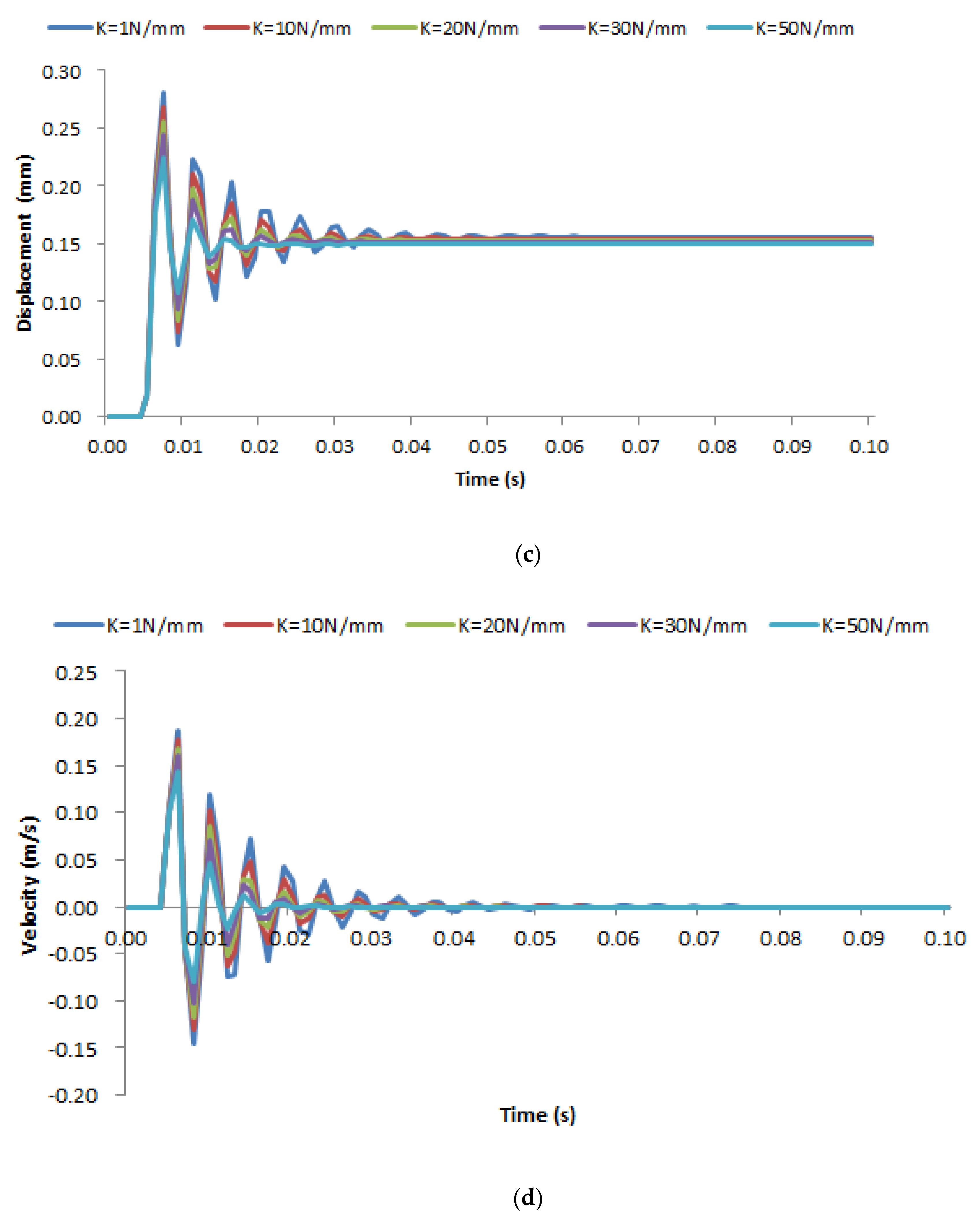
Figure 14.
(a) The pressure response characteristics—oil sealing length: 0~2 mm. (b) The flowrate response characteristics—oil sealing length: 0~2 mm. (c) The displacement response characteristics—oil sealing length: 0~2 mm. (d) The velocity response characteristics—oil sealing length: 0~2 mm.
Figure 14.
(a) The pressure response characteristics—oil sealing length: 0~2 mm. (b) The flowrate response characteristics—oil sealing length: 0~2 mm. (c) The displacement response characteristics—oil sealing length: 0~2 mm. (d) The velocity response characteristics—oil sealing length: 0~2 mm.
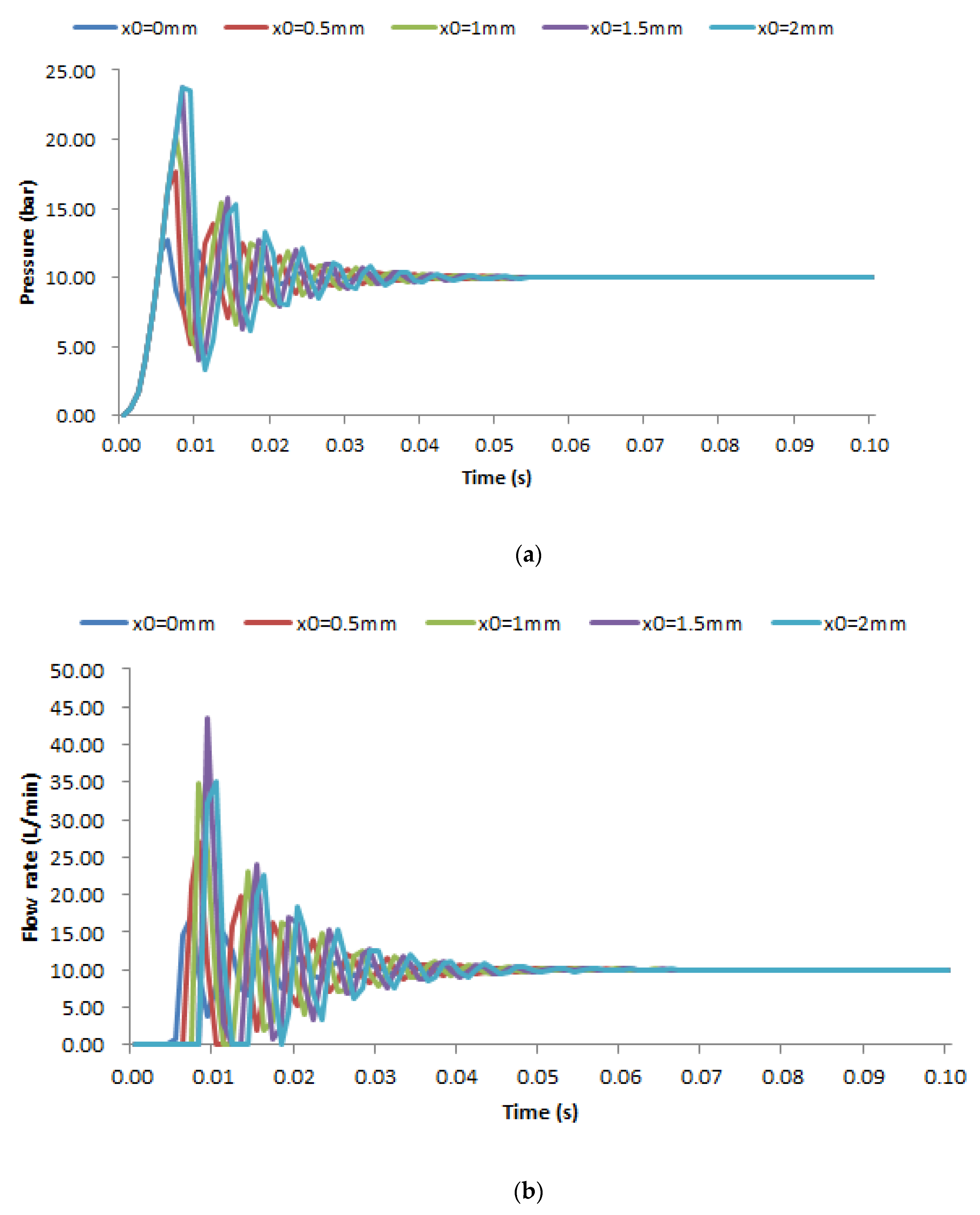

Figure 15.
(a) The pressure response characteristics—valve element diameter: 10~15 mm. (b) The flowrate response characteristics—valve element diameter: 10~15 mm. (c) The displacement response characteristics—valve element diameter: 10~15 mm. (d) The velocity response characteristics—valve element diameter: 10~15 mm.


Table 1.
Simulation parameters—group 1.
| Orifice Diameter | Viscosity Coefficient | Valve Element Mass | Spring Stiffness | Oil Seal Length | Valve Element Diameter |
|---|---|---|---|---|---|
| (mm) | (N/(m/s)) | (kg) | (N/mm) | (mm) | (mm) |
| 1~4 | 100 | 0.01 | 1 | 0 | 10 |
Table 2.
Simulation parameters—group 2.
| Orifice Diameter | Viscosity Coefficient | Valve Element Mass | Spring Stiffness | Oil Seal Length | Valve Element Diameter |
|---|---|---|---|---|---|
| (mm) | (N/(m/s)) | (kg) | (N/mm) | (mm) | (mm) |
| 2 | 40~60 | 0.01 | 1 | 0 | 10 |
Table 3.
Simulation parameters—group 3.
| Orifice Diameter | Viscosity Coefficient | Valve Element Mass | Spring Stiffness | Oil Seal Length | Valve Element Diameter |
|---|---|---|---|---|---|
| (mm) | (N/(m/s)) | (kg) | (N/mm) | (mm) | (mm) |
| 2 | 100 | 0.01~0.03 | 1 | 0 | 10 |
Table 4.
Simulation parameters—group 4.
| Orifice Diameter | Viscosity Coefficient | Valve Element Mass | Spring Stiffness | Oil Seal Length | Valve Element Diameter |
|---|---|---|---|---|---|
| (mm) | (N/(m/s)) | (kg) | (N/mm) | (mm) | (mm) |
| 2 | 100 | 0.013 | 1,10,20,30,50 | 0 | 10 |
Table 5.
Simulation parameters—group 5.
| Orifice Diameter | Viscosity Coefficient | Valve Element Mass | Spring Stiffness | Oil Seal Length | Valve Element Diameter |
|---|---|---|---|---|---|
| (mm) | (N/(m/s)) | (kg) | (N/mm) | (mm) | (mm) |
| 2 | 100 | 0.013 | 1 | 0~2 | 10 |
Table 6.
Simulation parameters—group 6.
| Orifice Diameter | Viscosity Coefficient | Valve Element Mass | Spring Stiffness | Oil Seal Length | Valve Element Diameter |
|---|---|---|---|---|---|
| (mm) | (N/(m/s)) | (kg) | (N/mm) | (mm) | (mm) |
| 2 | 100 | 0.013 | 1 | 0 | 10~15 |
Disclaimer/Publisher’s Note: The statements, opinions and data contained in all publications are solely those of the individual author(s) and contributor(s) and not of MDPI and/or the editor(s). MDPI and/or the editor(s) disclaim responsibility for any injury to people or property resulting from any ideas, methods, instructions or products referred to in the content. |
© 2023 by the authors. Licensee MDPI, Basel, Switzerland. This article is an open access article distributed under the terms and conditions of the Creative Commons Attribution (CC BY) license (https://creativecommons.org/licenses/by/4.0/).
Share and Cite
MDPI and ACS Style
Liu, H.; Zhao, Q. Study on the Influencing Factors of the Response Characteristics of the Slide Valve-Type Direct-Acting Relief Valve with External Orifice. Processes 2023, 11, 397. https://doi.org/10.3390/pr11020397
AMA Style
Liu H, Zhao Q. Study on the Influencing Factors of the Response Characteristics of the Slide Valve-Type Direct-Acting Relief Valve with External Orifice. Processes. 2023; 11(2):397. https://doi.org/10.3390/pr11020397
Chicago/Turabian StyleLiu, Huiyong, and Qing Zhao. 2023. "Study on the Influencing Factors of the Response Characteristics of the Slide Valve-Type Direct-Acting Relief Valve with External Orifice" Processes 11, no. 2: 397. https://doi.org/10.3390/pr11020397
Note that from the first issue of 2016, this journal uses article numbers instead of page numbers. See further details here.