
Distribution System State Estimation Based on Enhanced Kernel Ridge Regression and Ensemble Empirical Mode Decomposition


College of Mechanical Engineering and Automation, Liaoning University of Technology, Jinzhou 121001, China
*
Author to whom correspondence should be addressed.
Processes 2024, 12(4), 823; https://doi.org/10.3390/pr12040823
Submission received: 3 March 2024
/
Revised: 15 April 2024
/
Accepted: 16 April 2024
/
Published: 19 April 2024
(This article belongs to the Topic Advanced Operation, Control, and Planning of Intelligent Energy Systems)
Abstract
:In the case of strong non-Gaussian noise in the measurement information of the distribution network, the strong non-Gaussian noise significantly interferes with the filtering accuracy of the state estimation model based on deep learning. To address this issue, this paper proposes an enhanced kernel ridge regression state estimation method based on ensemble empirical mode decomposition. Initially, ensemble empirical mode decomposition is employed to eliminate most of the noise data in the measurement information, ensuring the reliability of the data for subsequent filtering. Subsequently, the enhanced kernel ridge regression state estimation model is constructed to establish the mapping relationship between the measured data and the estimation residuals. By inputting the measured data, both estimation results and estimation residuals can be obtained. Finally, numerical simulations conducted on the standard IEEE-33 node system and a 78-node system in a specific city demonstrate that the proposed method exhibits high accuracy and robustness in the presence of strong non-Gaussian noise interference.
1. Introduction
With the integration of large-scale renewable energy sources, it is essential to integrate and process the data information in the distribution network to improve security, reliability, and efficiency. These functions are implemented based on the distribution management system (DMS), which can monitor, protect, and control the whole distribution system [1]. As an important part of the DMS, state estimation utilizes real-time measurement information collected by supervisory control and data acquisition (SCADA) and the Wide-area Measurement System (WMS) to estimate the state of the system [2]. The essence of state estimation is the process of mapping measurement information to state variables [3]. Currently, most measurement information is collected from SCADA. However, during the data collection and transmission processes, the measurement information will inevitably be affected by measurement noise and transmission noise, resulting in the inclusion of abnormal data in the measurement information, which significantly affects the accuracy of state estimation. In [4], a detailed overview of the current mainstream state estimation methods, future challenges, and development prospects is provided. However, in the research on distribution network state estimation, how to handle non-Gaussian noise and improve the accuracy of filtering models remains a key issue that urgently needs to be addressed.
Forecasting-aided state estimation (FASE) takes into account the state transition characteristics of the system over time and can reflect the essence of quasi-steady state changes in the power system [5]. With the rapid development of modern information technology, the performance of FASE has been effectively improved, and it can provide prediction data for multiple samples at each time step. While state estimation based on the Kalman filter can effectively address filtering problems in linear systems, it is challenging to apply directly to nonlinear systems [6]. Consequently, a series of improved algorithms based on the Kalman filter have been proposed to address the FASE problem in nonlinear systems [7]. In [8], the extended Kalman filter algorithm is used to perform a Taylor series expansion of the nonlinear measurement equation to achieve linearization of the state estimation model. In [9], a state transition model based on Holt’s two-parameter exponential smoothing method is proposed, which reduces the prediction deviation caused by load transients. Building on Holt’s method, a sliding surface-enhanced fuzzy control FASE model is proposed in [10], which combines fuzzy mathematics with the extended Kalman filter algorithm to mitigate the negative impacts of load transients on state estimation. In [11], to enhance the robustness of state estimation, an exponential function weight function is formulated using the absolute residual vector, which improves the robustness of the filtering model.
The above models are still essentially first-order Taylor series approximations of nonlinear models, which ignore the influence of higher-order components, leading to biases in the filtering results. The unscented Kalman filter (UKF) is another commonly used nonlinear state estimation model that uses the unscented transformation to solve the mean and covariance matrix to achieve an approximation of nonlinear models [12,13]. However, this method is sensitive to non-Gaussian noise. To further improve estimation performance, a series of state estimation methods based on deep neural networks have gradually been applied to the power system [14]. In [15], the KRR-UKF is used in state estimation, which can be applied without considering the actual physical model. It filters unknown measurements in the power system, thereby improving system accuracy, but it does not consider the economic aspects of system operation in practical applications. In [16], a robust adaptive unscented Kalman filter is proposed, which can detect and identify gross errors and improve the robustness of UKF. In [17,18], the particle filter is integrated with long short-term memory (LSTM), and a power flow calculation is conducted based on pseudo-measurements predicted by LSTM to complement the missing state quantities, thereby enhancing the robustness and accuracy of state estimation.
Due to the low redundancy of measurements in the distribution network, it is necessary to use pseudo-measurements to ensure the observability of the system [19]. In [20], the node injection power and branch power are equivalently converted into current measurements, which improves the accuracy of state estimation. However, as the Jacobian matrix still needs to be updated in each iteration, the estimation efficiency of this method is relatively low. A distributed multi-agent-based method is proposed in [21] to deal with the complexity of active distribution networks by using an artificial bee colony algorithm, which improves the efficiency of state estimation. In [22], the iterative procedure of Broyden’s rank-one update is used to approximate the time-varying process and measurement Jacobian matrices in EKF, which can significantly reduce the computation time. In [23], particle filtering is combined with a convolutional neural network for state estimation, which effectively improves the accuracy of state estimation. In [24], kernel ridge regression is used to handle uncertainty in the system, improving the accuracy of state estimation after collecting a large amount of measurement data. However, in practical applications, the presence of non-Gaussian noise can reduce the accuracy of system state estimation. Further research is needed to investigate how to handle non-Gaussian noise in measurement information. In [25], a robust cubature particle filter algorithm is proposed by integrating multiple time-scale factors with the traditional cubature particle filter algorithm, which effectively enhances the estimation performance of the system, especially in the presence of non-Gaussian measurement noise.
The enhanced kernel ridge regression state estimation (EKRRSE) method for distribution network state estimation based on ensemble empirical mode decomposition (EEMD) is introduced in this study. The main problems addressed are as follows:
(1) To solve the problem of the increased estimation error of KRRSE caused by measurement noise, EEMD is employed to suppress the noise in measurement data to improve the filtering effect of KRRSE.
(2) Kernel ridge regression is used to express the mapping relationship between measurement data and the estimation error to further improve the estimation accuracy.
2. Ensemble Empirical Mode Decomposition and Enhanced Kernel Ridge Regression Filtering
2.1. Measurement Noise Reduction Based on EEMD
EEMD separates multiple intrinsic mode functions (IMFs) and a residual component function from the original measurement, where each IMF represents the dynamic variation pattern at a specific instantaneous frequency, highlighting the local features of the measurement data, while the residual component reflects the overall trend of the measurement data. Decomposing the measurement data using EEMD involves first calculating all the extreme points of the measurement data . Next, the upper and lower envelopes of the original measurement are obtained through cubic spline interpolation, and the mean value curve of these envelopes is computed; then a new denoised measurement component , which excludes low frequencies, is obtained as follows:
If a component satisfies the condition where the number of extreme points and zero-crossing points in the entire measurement data is equal or differs by at most one, and the average of the upper and lower envelopes determined by cubic spline interpolation is zero, then is considered the first-order IMF of the measurement data . Otherwise, is taken as an input, and the above steps are repeated as follows:
where is an intermediate variable, and is the mean curve of the upper and lower envelopes obtained by cubic spline interpolation on . It is worth noting that abnormal data collected by the measurement system can impact the partitioning of the upper and lower envelopes and the decomposition results. Therefore, an outlier handling method is needed to deal with the abnormal data. It is assumed that, after k iterations, the first-order IMF component and the remaining component of the measurement information are as follows:
If we make this assumption, we can continue the above operation on until the remaining component is a monotonic function, which can be expressed as follows:
where represents the nth-order residual component. As a result, the original measurement data can be expressed as the sum of several IMF components and the final residual component .
The above decomposition process exhibits good adaptability to input data. However, in the presence of noise in the measurement data, rapid fluctuations in extremum values may occur within an extremely short period. This can cause a single IMF to encompass time-scale features with significant differences, leading to a mode-mixing problem where a single IMF reflects multiple characteristics of the measurement data. To solve this problem, the Gaussian white noise with a mean of 0 is added to the original measurement , resulting in processed measurement data . This helps mask the original noise in the measurement data.
Empirical mode decomposition is then conducted on , yielding the following:
Then, we add white noise with a mean of 0 to the original measurement information , respectively, repeat the operations described by Equations (5) and (6), and obtain the decomposition results of the measurement information under different levels of white noise.
where represents the white noise added in the i-th iteration, and as a result, is the corresponding IMF component. Considering the mean value of the Gaussian noise is 0, ensemble averaging is performed on the IMF components, and we obtain the following:
where m represents the number of times Gaussian white noise is added.
The difference between the measured information and the sum of the final IMF components can be expressed as follows:
where represents the amplitude of the white noise.
It can be seen from (11) that, with a constant amplitude of white noise, the more times noise is added, the closer the sum of the IMF components is to the original data. The final result of the measured information decomposition can be expressed as follows:
Due to the strong temporal characteristics of the measurement information and the random distribution of the unknown noise, the noise components with high temporal complexity in the measurement information can be identified by calculating the sample entropy coefficients of each IMF of the original measurement [26], thereby achieving noise reduction in the measured information. First, the IMF components of the measurement information in (10) are arranged in a vector sequence.
The distance between and is defined as d, the absolute value of the maximum difference of the corresponding elements of their respective IMF components.
where , , , and . For a given , the ratio of the number of instances where the distance between and is less than the specified similarity tolerance to the total number of components is denoted as .
The mean value of is as follows:
We increase the dimension to and similarly calculate the ratio and the mean value.
Therefore, the sample entropy of this sequence is as follows:
When m takes a finite value, we have the following:
where n is the embedding dimension and r is the similarity tolerance.
2.2. Enhanced Kernel Ridge Regression
To further reduce estimation errors, KRRSE is used to learn the discrepancy between the actual state and the estimated state information. The KRRSE state estimation model is defined as follows:
where represents the estimation results of the kernel ridge regression model, and the corresponding dataset is . is the estimation residual. It is evident that the key to improving the filtering effect lies in reducing the estimation residual. Considering that the error data of the output of the KRRSE model contain the distribution rules of unknown noise, kernel ridge regression is used to learn the nonlinear relationship between the estimation results and the real estimation model . The state estimation model is represented as follows:
where and represent the input measurements, and represents the error of the KRRSE model. The noise . The enhanced kernel ridge regression algorithm effectively improves the estimation performance by learning the noise distribution in the data and updating the weights of the model parameters.
3. State Estimation of Distribution System Based on EEMD-EKRRSE
3.1. Density-Based Spatial Clustering of Applications with Noise
The primary step in handling abnormal data is to determine whether the current input data contain any adverse information. Considering the large scale of historical measurement data in distribution networks, traditional residual identification search methods are inefficient. Therefore, in this section, density-based spatial clustering of applications with noise (DBSCAN) is adopted to classify errors and missing data in the measurement data. To use the clustering algorithm, the following definitions are provided first:
(1) Domain : For any input measurement data , the interior region of a circular area with a center and a radius is referred to as the domain . The collection of all measurement information within this domain is as follows:
(2) Core Target: For any measurement datum , if the number of measurement information sets corresponding to the domain exceeds the value of , then the measurement datum is considered a core target.
(3) Direct Density Reachable: If two measurement data points and are core targets, and is located within the domain of , then is said to be density reachable from . When is also a core target, it is also considered density reachable from .
(4) Density Reachable: For multiple measurement data points , if is density reachable from , then is considered density reachable from .
(5) Density Connected: If three measurement data points , where and are both density reachable from the core object , then and are considered density connected.
When the measurement data are input into DBSCAN, the clustering algorithm will mark multiple core objects in the measurement data based on the set domain radius and the minimum number of points required to form a core object within the domain radius . The core object set is established, and data points near core objects that have fewer than points within the domain radius are temporarily marked as outliers. After traversing all measurement data, the detection process for outliers is completed.
3.2. Convolutional Neural Network Based on Attention Mechanism Combined with Gated Recurrent Unit
The measurement data are influenced by meteorological factors and time, thus exhibiting a temporal pattern of change. Time-series forecasting algorithms can be used to explore the temporal characteristics of historical measurements and construct reliable pseudo-measurement data.
(1) Attention Mechanism: The research objective of the attention mechanism is to intelligently allocate weights to the data. By calculating the influence weights of individual input data, abstracting the weight information of historical time-series data, and averaging all information weight factors through weighted averaging, adaptive weight distribution can be achieved.
Taking the measurement information as an example, let us denote the historical measurement data from time 1 to n − 1 as . First, we use a scoring function, denoted as , as follows:
where , , and are weights that are automatically updated through learning, and tanh represents the hyperbolic tangent function, used to compute the correlation between each historical measurement datum and the measurement datum at time n. The computed results are then normalized using the normalization exponential function to obtain the attention distribution among all historical measurement inputs , with the following calculation formula:
where exp represents the exponential function. According to Equation (26), the attention distribution obtained is used to perform a weighted sum of historical measurement data, resulting in the relevant input information to be considered.
(2) Convolutional Neural Network: Given the large volume of historical measurement data, the model parameters also increase with the data volume, which can lead to overfitting or training difficulties in neural networks, causing the problem of parameter explosion when predicting measurement information. Convolutional neural networks (CNN), however, can address this issue by using pooling and convolution to process data, enabling local connections and weight sharing to mitigate problems such as parameter explosion.
Compared to the fully connected architecture of traditional neural networks, convolutional neural networks employ a partial connectivity approach when connecting upper-layer neurons to the convolutional layers, extracting partial features of the input information. Additionally, within the same layer, CNNs classify neurons based on the strength of their connections, assigning corresponding weight values to neurons of the same type with the same convolutional kernel. This is expressed in Equation (28):
where represents the output matrix of the convolution operation, denotes the activation function of the convolutional layer, signifies the input information of the -th window in layer , and , respectively, represent the weight parameter matrix and bias parameter matrix of the input information, and indicates the position of the tensor containing the extracted partial data features.
To further reduce the data size and network parameters, a pooling layer is added after the convolutional layer in the convolutional neural network. Its expression is as follows:
where represents the output matrix of the pooling layer, is the max pooling function, denotes the input information corresponding to the -th convolutional kernel of layer , and represents the sampling kernel.
After the original data undergo feature refinement in the convolutional layer and feature selection in the pooling layer, they are then fused through the fully connected layer to integrate the deep-level data features of each locality. The principle is demonstrated in Equation (30):
where represents the output of the fully connected layer, is the activation function of the fully connected layer, is the input to the entire layer , and and are the weight parameters and bias parameters of the fully connected layer, respectively.
3.3. Ensemble Empirical Mode Decomposition-Enhanced Kernel Ridge Regression State Estimation
To address the issue of significant errors in KRRSE filtering under intense non-Gaussian noise, an enhanced kernel ridge regression state estimation method, referred to as ensemble empirical mode decomposition (EEMD-EKRRSE), is proposed in this paper. EEMD is utilized to remove noise from the measurements and diminish the impact of measurement noise on the data. Furthermore, the kernel ridge regression method is employed to model the nonlinear mapping relationship between the measured information and estimation residuals. The estimation process of EEMD-EKRRSE is depicted in Figure 1, encompassing the following primary steps.
Step 1: Model training. The Convolutional Neural Network Based on Attention Mechanism Combined with Gated Recurrent Unit (CAGN) is utilized to learn the temporal patterns in historical measurement data. Kernel ridge regression state estimation (KRRSE) is employed to learn the mapping relationships between measurement data and state information, as well as between measurement data and estimation residuals, thereby establishing the EEMD-EKRRSE model.
Step 2: Detection of anomalies and missing data. The missing or anomalous data in the measurement dataset are determined using the DBSCAN method. If anomalies are detected, proceed to Step 3; if the data are normal, proceed to Step 4.
Step 3: Handling of anomalous data. The CAGN model established in Step 1 is utilized to reconstruct the measurement data, and the dataset containing the reconstructed data is fed into the EKRRSE filtering model.
Step 4: Processing of Normal Data. The normal measurement data are denoised using EEMD and then fed into the EKRRSE filtering model, and the final state estimation results are obtained.
4. Case Studies
The effectiveness of the proposed EEMD-EKRRSE method is verified on the IEEE-33 node system and a 78-node distribution system in China. The test is performed on a PC purchased in Qingdao, Shandong, China, produced by HP, with Intel Core i5-9300, 16 GB of RAM. The relevant algorithms are compiled using the Python platform 3.6. The CNN model and the kernel ridge regression model are trained using the TensorFlow 2.10.0 and Keras 2.10.0 toolboxes, respectively. The MATPOWER 7.0 toolbox is employed to obtain the system state dataset and measurement dataset through power flow calculations.
4.1. IEEE-33 Node System
(1) Measurement Denoising Effect
To analyze the impact of strong non-Gaussian noise, Laplace noise with a mean of 0 and a standard deviation of 0.01, and Gaussian noise with a weight of 0.5, and a weight of 0.5, both with covariances of 10−5I and 10−3I, are added to the measurement data of node 4, respectively. The EEMD decomposition is used to decompose the original measurement into multiple IMF components. Under the interference of these two types of noise, EEMD decomposition is performed on 1000 sets of active power and reactive power measurement data. The results are shown in Table 1 and Figure 2.
From Table 1, it can be observed that the IMF1 component has the highest sample entropy for both active and reactive power, indicating the highest time-series complexity of this component.
From Figure 2, it can be seen that the distribution characteristics of each IMF component are significantly different. After removing the IMF1 component, the denoised measurement data can be obtained. Table 2 and Figure 3 show the Absolute Error (AE) and Root Mean Square Error (RMSE) of 1000 sets of active power and reactive power measurements at this node before and after denoising.
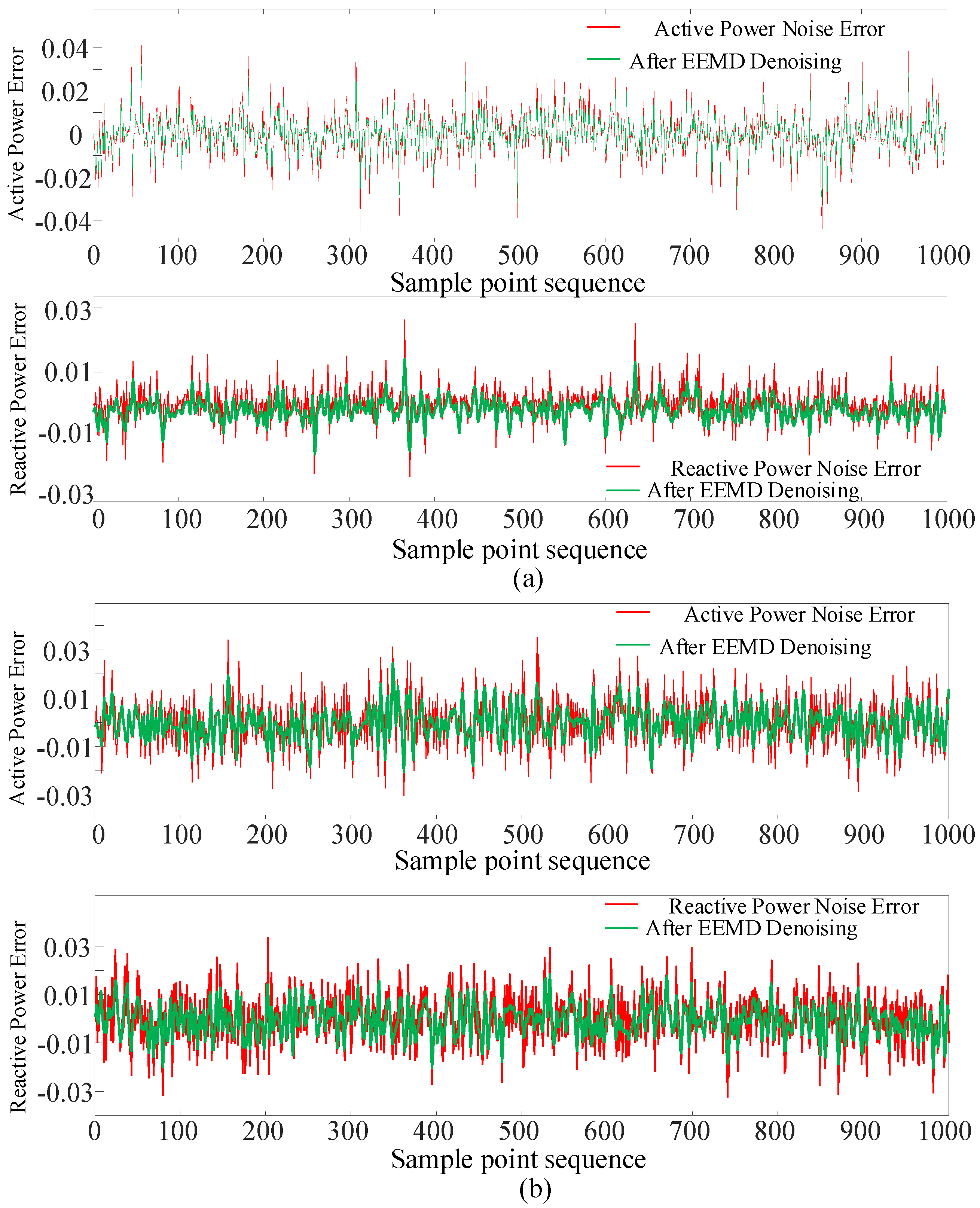
From Table 2, it can be seen that in the Laplace noise environment, the absolute errors of active power and reactive power after denoising using EEMD are 6.74 × 10⁻³ and 6.58 × 10⁻³, respectively, which are reduced by 6.5% and 35% compared to the errors before denoising. In the bimodal Gaussian noise environment, the absolute errors of active power and reactive power are reduced by 38% and 35%, respectively. Moreover, the RMSE of active power and reactive power in the Laplace noise environment is reduced by 8% and 30%, respectively, compared to the RMSE before denoising. In the bimodal Gaussian noise environment, they are reduced by 36% and 35%, respectively. It can be seen that EEMD has a significant noise reduction effect.
From Figure 3, it can be observed that the fluctuation amplitude of the error curve of the denoised measurement information using EEMD is significantly reduced, indicating that EEMD can effectively reduce the noise level in the measurement information. To further demonstrate the denoising effect of EEMD under strong non-Gaussian noise, Laplace noise with a mean of 0 and standard deviation ranging from 0.02 to 0.05 with a step of 0.01 is added to the active power data of node 4, and EEMD is then used to denoise the data.
Table 3 shows that the AE and RMSE after denoising using EEMD decreased by 27% and 33% on average, respectively, indicating that the denoised measurement data are closer to the true values. This validates the denoising effect of EEMD under strong non-Gaussian noise.
(2) Filtering Effect of EKRRSE
Laplace noise with a mean of 0 and standard deviation ranging from 0.01 to 0.05 in increments of 0.01 is added to the measurement data at node 4, and KRRSE is then used to filter. Table 4 presents the results of the Mean Absolute Percentage Error (MAPE) and RMSE of KRRSE. Additionally, Figure 4 illustrates the comparison of filtering performance before and after denoising with EEMD when the noise deviation is 0.05.
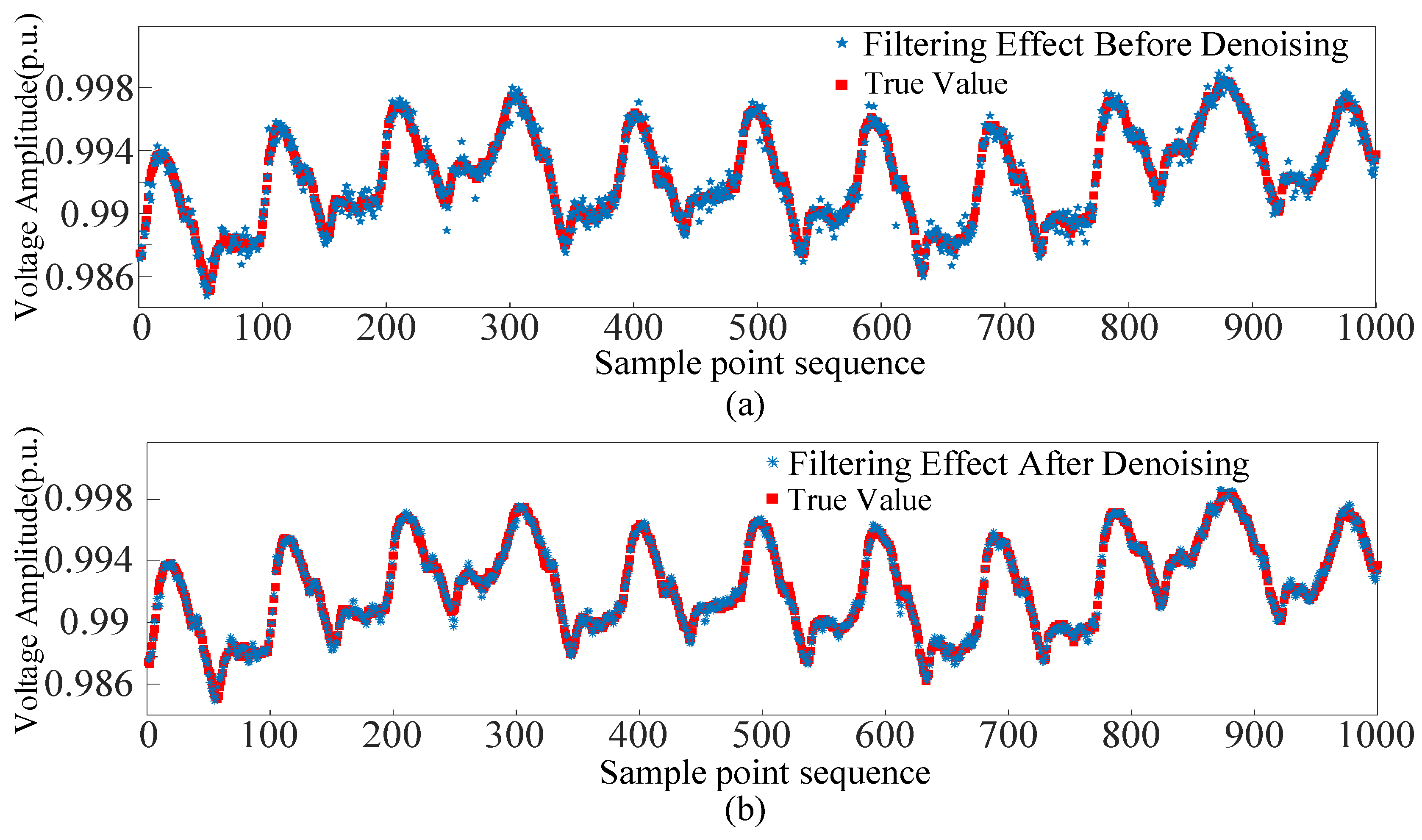
From Table 4, it can be seen that before denoising, as the standard deviation of noise increases, the MAPE of KRRSE filtering gradually increases. When the noise standard deviation increases from 0.01 to 0.05, the MAPE and RMSE increase by 3.56 times and 3.77 times, respectively, showing a significant decrease in filtering performance. However, after noise reduction by EEMD, the MAPE is reduced by nearly 29% on average, and the filtering accuracy is significantly improved. When the noise standard deviation is 0.05, the RMSE is 3.28 × 10⁻⁴, which is 33% lower than before denoising, enhancing filtering stability. From Figure 4, it is evident that the filtering values before denoising deviate from the true value at multiple points, which is more obvious at the peak and valley points of the curve. After denoising with EEMD, the data errors are reduced, and the measured information is closer to the true values. Consequently, KRRSE shows improved filtering performance, validating that EEMD-based measurement denoising effectively improves the accuracy and stability of KRRSE filtering.
To further reduce the estimation errors, the nonlinear relationship between the measurement information and the estimation residuals is learned through kernel ridge regression, and the estimated residuals are then integrated into the results of the first-stage filtering.
To validate the effectiveness of the EKRRSE method, we take node 4 as an example. Laplace noise with a mean of 0 and standard deviation ranging from 0.01 to 0.05 in steps of 0.01 is superimposed onto the measurement data of node 4. The EKRRSE method is then used to filter the denoised measurement data.
Table 5 presents a comparison of the filtering effects between KRRSE and EKRRSE. It can be seen that under the influence of noise with different standard deviations, compared to the filtering results of KRRSE, EKRRSE shows a decrease in both MAPE and RMSE. Specifically, the MAPE decreases by 8.4% on average, and the RMSE decreases by 9.3% on average. This indicates that EKRRSE can improve the estimation accuracy and stability, making the filtering results closer to the true values.
(3) Robustness Analysis
DBSCAN is used to filter the abnormal data in measurements, and CAGN is utilized to reconstruct the corresponding measurement data. It is worth noting that the reconstructed measurement information obtained by CAGN has high accuracy, and EEMD is not suitable for denoising the reconstructed information. EKRRSE is applied to handle the reconstructed measurement information to improve the filtering effect. To evaluate the filtering performance of EKRRSE on abnormal data, two scenarios are studied, and the filtering results of KRRSE and EKRRSE are compared as shown in Table 6.
Scenario 1: The active power measurement information for nodes 12 and 32 is missing from sample point 3 to sample point 70.
Scenario 2: The reactive power measurement information for nodes 15 and 23 is abnormal from sample point 3 to sample point 70.
From Table 6, it can be observed that the MAPE and RMSE of EKRRSE in Scenarios 1 and 2 are both lower than those of KRRSE. The accuracy and estimation stability of EKRRSE are better than KRRSE overall. This is because EKRRSE can learn the mapping relationship between the reconstructed measurement information and the residuals, further reducing the estimation residuals and improving the filtering accuracy of the algorithm in abnormal scenarios.
(4) Computation Efficiency
The performance of EKRRSE, KRRSE, Cubature Particle Filter (CPF) [25], and Robust Cubature Particle Filter (RCPF) [25] in terms of computation efficiency and error are compared, and the results are shown in Table 7.
From Table 7, it can be observed that EKRRSE exhibits the highest accuracy. This is attributed to the algorithm’s ability to utilize the estimation residuals effectively, thereby improving the filtering accuracy. As the EKRRSE filtering model requires additional training of residual information, the runtime has slightly increased but still remains within the millisecond level. Therefore, the proposed EKRRSE method in this paper meets the requirements for both computation efficiency and accuracy in state estimation.
4.2. A 78-Node System
To further validate the effectiveness of the proposed EEMD-EKRRSE method, a case study is conducted on a 78-node distribution system in China.
(1) Measurement Denoising Effect
Laplace noise with a mean of 0 and a standard deviation of 0.01, and bimodal Gaussian noise with covariance matrices of 10−5I and 10−3I and weights of 0.5 for each mode, are added to the active and reactive power data of node 17 of this system. The original measurements are decomposed into multiple IMF components using EEMD, and the reconstruction results are shown in Table 8 and Figure 5.
After EEMD denoising, the AE of the active power decreased from 6.68 × 10⁻³ to 5.87 × 10⁻³, and the AE of the reactive power decreased from 7.31 × 10⁻³ to 6.09 × 10⁻³ in the Laplace noise environment, reducing by approximately 12% and 17%, respectively. In the bimodal Gaussian noise environment, the AE of the active power is reduced by nearly 20% and the AE of the reactive power is reduced by about 19%, demonstrating a significant denoising effect.
As shown in Figure 5, the RMSE of each denoised measurement is obviously reduced. To demonstrate the denoising effect of EEMD under strong non-Gaussian noise, Laplace noise with a mean of 0 and standard deviation ranging from 0.02 to 0.05 in steps of 0.01 is superimposed onto the active power data of node 17, and EEMD is used to denoise the data. Table 9 shows the comparison of measurement errors before and after denoising.
From Table 9, it can be seen that under the influence of gradually increasing noise, the error after denoising with EEMD is always lower than the original error. Specifically, AE is reduced by nearly 29%, indicating that the denoised data are closer to the true measurement. RMSE is decreased by nearly 38%, improving the stability of measurement data and ensuring the reliability and accuracy of the data required for subsequent filtering.
(2) Effect of EKRRSE Filtering after Denoising
To verify the denoising effect of EEMD decomposition, Laplace noise with a mean of 0 and standard deviations ranging from 0.01 to 0.05 in steps of 0.01 is superimposed onto the measurement data of node 17. Subsequently, EEMD-denoised measurements are filtered using EKRRSE, and the results are presented in Table 10.
Table 10 shows that EKRRSE can also improve the filtering effect in the practical distribution system. The average MAPE is decreased by 15%, and the average RMSE is decreased by 14%, further improving the filtering accuracy and stability. This is because EKRRSE can obtain the relative weights of each regression independent variable on the state information, and establish a mapping relationship between measurement and residuals, thereby obtaining more reliable estimated residuals.
(3) Robustness Analysis
Table 11 shows a comparison of the filtering results between EKRRSE and KRRSE to evaluate the filtering performance on abnormal data. Two scenarios are considered to compare the filtering results.
Scenario 1: The active power measurement information of nodes 11 and 61 randomly deviates from the normal value by 50%.
Scenario 2: 20% of the reactive power measurement information of nodes 8 and 10 is missing randomly.
Table 11 shows that the MAPE and RMSE of EKRRSE are lower than those of KRRSE. This is because EKRRSE learns the relationship between measurement information and residual errors, making the filtering results closer to the true state and improving filtering accuracy and stability.
(4) Computation Efficiency
To further validate the performance advantages of the proposed EKRRSE method, a comparison between EKRRSE and KRRSE is conducted in terms of the runtime and relative error. The results are presented in Table 12.
From Table 12, it can be observed that EKRRSE has a slightly increased runtime due to the integration of residual information from KRRSE. However, it still remains within the millisecond range. In addition, the relative error of EKRRSE is lower than that of KRRSE, improving the filtering performance. This demonstrates that the EKRRSE method also exhibits high efficiency and accuracy in practical distribution systems.
5. Conclusions
This paper introduces the EEMD method to separate noise data from measurement information and refine measurement data. As for the filtering model, an optimization method based on an approximate model is employed to reduce the gap between the filtering model and the real model. The EEMD-EKRRSE filtering model is established, further enhancing the effectiveness and accuracy of the filter. Extensive case studies are conducted on the IEEE-33 and a 78-node distribution network in a certain city, leading to the following main conclusions:
- (1)
- EEMD-based denoising can effectively reduce the error of measurement, make the measurement data closer to true values, and provide more reliable measurement data for subsequent filtering.
- (2)
- The proposed EKRRSE state estimation model could efficiently learn the mapping relationship between measurement information and residuals during the training process, improving filtering accuracy and stability.
- (3)
- The uncertainty of the distributed generation output inevitably leads to variations in the state estimation results. Therefore, in the future, a quantitative analysis of the DG output can be conducted to more accurately assess its impact on state estimation, thereby comprehensively improving the reliability of state estimation.
Author Contributions
Conceptualization, X.C.; methodology, X.C.; software, J.W.; validation, X.C.; formal analysis, X.C.; investigation, X.C.; resources, X.C.; data curation, J.W.; writing—original draft preparation, X.C.; writing—review and editing, J.W.; visualization, X.C.; supervision, X.C.; project administration, X.C.; funding acquisition, X.C. All authors have read and agreed to the published version of the manuscript.
Funding
This research was funded by the Science Research Funding Project of the Education Department of Liaoning Province (No. LJKZ0603), Doctoral Research Start-up Fund Project of Liaoning Province (No. 2022-BS-308).
Data Availability Statement
The data presented in this study are available on request from the corresponding author.
Conflicts of Interest
The authors declare no conflicts of interest.
References
- Hossan, M.S.; Chowdhury, B. Integrated CVR and demand response framework for advanced distribution management systems. IEEE Trans. Sustain. Energy 2019, 11, 534–544. [Google Scholar] [CrossRef]
- Maseda, F.J.; López, I.; Martija, I.; Alkorta, P.; Garrido, A.J.; Garrido, I. Sensors data analysis in supervisory control and data acquisition (SCADA) systems to foresee failures with an undetermined origin. Sensors 2021, 21, 2762. [Google Scholar] [CrossRef] [PubMed]
- Li, Z.; Xu, Y.; Wu, L.; Zheng, X. A risk-averse adaptively stochastic method for multi-energy ship operation under diverse uncertainties. IEEE Trans. Power Syst. 2020, 36, 2149–2161. [Google Scholar] [CrossRef]
- Fotopoulou, M.; Petridis, S.; Karachalios, I.; Rakopoulos, D. A review on distribution system state estimation algorithms. Appl. Sci. 2022, 12, 11073. [Google Scholar] [CrossRef]
- Li, J.; Gao, M.; Liu, B.; Cai, Y. Forecasting Aided Distribution Network State Estimation Using Mixed μPMU-RTU Measurements. IEEE Syst. J. 2022, 16, 6524–6534. [Google Scholar] [CrossRef]
- Liu, H.; Hu, F.; Su, J.; Wei, X.; Qin, R. Comparisons on Kalman-filter-based dynamic state estimation algorithms of power systems. IEEE Access 2020, 8, 51035–51043. [Google Scholar] [CrossRef]
- Wang, K.; Liu, M.; He, W.; Zuo, C.; Wang, F. Koopman Kalman particle filter for dynamic state estimation of distribution system. IEEE Access 2022, 10, 111688–111703. [Google Scholar] [CrossRef]
- Beelen, H.; Bergveld, H.J.; Donkers, F. Joint estimation of battery parameters and state of charge using an extended Kalman filter: A single-parameter tuning approach. IEEE Trans. Control Syst. Technol. 2020, 29, 1087–1101. [Google Scholar] [CrossRef]
- Li, Z.; Xu, Y. Optimal coordinated energy dispatch of a multi-energy microgrid in grid-connected and islanded modes. Appl. Energy 2018, 210, 974–986. [Google Scholar] [CrossRef]
- Bilil, H.; Gharavi, H. MMSE-based analytical estimator for uncertain power system with limited number of measurements. IEEE Trans. Power Syst. 2018, 33, 5236–5247. [Google Scholar] [CrossRef]
- Rout, B.; Dahale, S.; Natarajan, B. Dynamic matrix completion based state estimation in distribution grids. IEEE Trans. Ind. Inform. 2022, 18, 7504–7511. [Google Scholar] [CrossRef]
- Zhu, F.; Fu, J. A novel state-of-health estimation for lithium-ion battery via unscented Kalman filter and improved unscented particle filter. IEEE Sens. J. 2021, 21, 25449–25456. [Google Scholar] [CrossRef]
- Wang, W.; Chi, K.T.; Wang, S. Dynamic State Estimation of Power Systems by p-Norm Nonlinear Kalman Filter. IEEE Trans. Circuits Syst. I Regul. Pap. 2020, 67, 1715–1728. [Google Scholar] [CrossRef]
- Gotti, D.; Amaris, H.; Larrea, P.L. A deep neural network approach for online topology identification in state estimation. IEEE Trans. Power Syst. 2021, 36, 5824–5833. [Google Scholar] [CrossRef]
- Zhang, W.; Zhang, S.; Zhang, Y.; Xu, G.; Mao, H. A KRR-UKF robust state estimation method for distribution networks. Front. Energy Res. 2023, 11, 1295070. [Google Scholar] [CrossRef]
- Zhang, Z.; Zhang, Z.; Zhao, S.; Li, Q.; Hong, Z.; Li, F.; Huang, F. Robust adaptive Unscented Kalman Filter with gross error detection and identification for power system forecasting-aided state estimation. J. Frankl. Inst. 2023, 360, 10297–10336. [Google Scholar] [CrossRef]
- Yu, Y.; Han, X.; Yang, M.; Yang, J. Probabilistic prediction of regional wind power based on spatiotemporal quantile regression. In Proceedings of the 2019 IEEE Industry Applications Society Annual Meeting, Baltimore, MD, USA, 29 September–3 October 2019. [Google Scholar]
- Ji, X.; Yin, Z.; Zhang, Y.; Wang, M.; Zhang, X.; Zhang, C.; Wang, D. Real-time robust forecasting-aided state estimation of power system based on data-driven models. Int. J. Electr. Power Energy Syst. 2021, 125, 106412. [Google Scholar] [CrossRef]
- Dehghanpour, K.; Wang, Z.; Wang, J.; Yuan, Y.; Bu, F. A survey on state estimation techniques and challenges in smart distribution systems. IEEE Trans. Smart Grid 2019, 10, 2312–2322. [Google Scholar] [CrossRef]
- Wang, H.; Schulz, N.N. A revised branch current-based distribution system state estimation algorithm and meter placement impact. IEEE Trans. Power Syst. 2004, 19, 207–213. [Google Scholar] [CrossRef]
- Adjerid, H.; Maouche, A.R. Multi-agent system-based decentralized state estimation method for active distribution networks. Comput. Electr. Eng. 2020, 86, 106652. [Google Scholar] [CrossRef]
- Mukherjee, T.; Varshney, D.; Kottakki, K.K.; Bhushan, M. Broyden’s update based extended Kalman Filter for nonlinear state estimation. J. Process Control 2021, 105, 267–282. [Google Scholar] [CrossRef]
- Li, M.; Li, C.; Zhang, Q.; Liao, W.; Rao, Z. State of charge estimation of Li-ion batteries based on deep learning methods and particle-swarm-optimized Kalman filter. J. Energy Storage 2023, 64, 107191. [Google Scholar] [CrossRef]
- Barati, M.; Ensaf, M.; Hosseini, B. Kernel Regression Method for Stochastic Real-time State Estimation in Power Grid. In Proceedings of the 2023 IEEE Kansas Power and Energy Conference (KPEC), Manhattan, KS, USA, 27–28 April 2023; pp. 1–5. [Google Scholar]
- Shi, Q.; Liu, M.; Hang, L. A novel distribution system state estimator based on robust cubature particle filter used for non-gaussian noise and bad data scenarios. IET Gener. Transm. Distrib. 2022, 16, 1385–1399. [Google Scholar] [CrossRef]
- Si, Z.; Yang, M.; Yu, Y.; Ding, T. Photovoltaic power forecast based on satellite images considering effects of solar position. Appl. Energy 2021, 302, 117514. [Google Scholar] [CrossRef]
Figure 1.
The flow chart of EMMD-EKRRSE.

Figure 2.
Results of EEMD under non-Gaussian noise. (a) EEMD decomposition of active power under Laplace noise. (b) EEMD decomposition of reactive power under Laplace noise. (c) EEMD decomposition of active power under bimodal Gaussian noise. (d) EEMD decomposition of reactive power under bimodal Gaussian noise.

Figure 3.
Denoise effects of measurements under non-Gaussian noise. (a) Comparison of measurement denoising under Laplace noise. (b) Comparison of measurement denoising under bimodal Gaussian Noise.
Figure 3.
Denoise effects of measurements under non-Gaussian noise. (a) Comparison of measurement denoising under Laplace noise. (b) Comparison of measurement denoising under bimodal Gaussian Noise.

Figure 4.
Comparison of filtering effect before and after noise reduction. (a) Filtering effect before denoising. (b) Filtering effect after denoising.
Figure 4.
Comparison of filtering effect before and after noise reduction. (a) Filtering effect before denoising. (b) Filtering effect after denoising.

Figure 5.
Denoise effects of measurements under non-Gaussian noise. (a) Comparison of measurement denoising under Laplace noise. (b) Comparison of measurement denoising under bimodal Gaussian noise.
Figure 5.
Denoise effects of measurements under non-Gaussian noise. (a) Comparison of measurement denoising under Laplace noise. (b) Comparison of measurement denoising under bimodal Gaussian noise.


Table 1.
IMF component sample entropy results.
| Components | Laplace Noise | Bimodal Gaussian Noise | ||
|---|---|---|---|---|
| Active Power (p.u.) | Reactive Power (p.u.) | Active Power (p.u.) | Reactive Power (p.u.) | |
| IMF1 | 2.48 | 2.32 | 2.36 | 2.19 |
| IMF2 | 1.91 | 2.09 | 1.88 | 2.07 |
| IMF3 | 1.14 | 1.08 | 1.03 | 1.14 |
| IMF4 | 0.633 | 0.638 | 0.670 | 0.694 |
| IMF5 | 0.542 | 0.511 | 0.515 | 0.600 |
| IMF6 | 0.442 | 0.470 | 0.469 | 0.454 |
| IMF7 | 0.129 | 0.119 | 0.129 | 0.132 |
| IMF8 | 0.0479 | 0.0457 | 0.0469 | 0.0457 |
| IMF9 | 0.00457 | 0.00408 | 0.00447 | 0.00449 |
| IMF10 | 0.00470 | 0.00463 | 0.00451 | 0.00494 |
| IMF11 | 0.00196 | 0.00176 | 0.00194 | 0.00392 |
Table 2.
Denoise effects of measurements under different non-Gaussian noise.
| Index | Laplace Noise | Bimodal Gaussian Noise | ||
|---|---|---|---|---|
| AE | RMSE | AE | RMSE | |
| Active power before denoising | 7.21 × 10⁻³ | 1.02 × 10⁻² | 7.92 × 10⁻³ | 9.92 × 10⁻³ |
| After EEMD denoising | 6.74 × 10⁻³ | 9.40 × 10⁻³ | 4.95 × 10⁻³ | 6.31 × 10⁻³ |
| Reactive power before denoising | 9.44 × 10⁻³ | 9.53 × 10⁻³ | 8.1 × 10⁻³ | 1.02 × 10⁻² |
| After EEMD denoising | 6.58 × 10⁻³ | 6.58 × 10⁻³ | 5.34 × 10⁻³ | 6.60 × 10⁻³ |
Table 3.
Denoise effects of measurements under non-Gaussian noise.
| Standard Deviation | Before Denoising | After Denoising by EEMD | ||
|---|---|---|---|---|
| AE | RMSE | AE | RMSE | |
| 0.02 | 2.91 × 10⁻² | 4.14 × 10⁻² | 2.56 × 10⁻² | 3.34 × 10⁻² |
| 0.03 | 3.48 × 10⁻² | 4.89 × 10⁻² | 2.51 × 10⁻² | 3.31 × 10⁻² |
| 0.04 | 3.62 × 10⁻² | 5.13 × 10⁻² | 2.90 × 10⁻² | 3.78 × 10⁻² |
| 0.05 | 3.80 × 10⁻² | 5.33 × 10⁻² | 2.05 × 10⁻² | 2.67 × 10⁻² |
Table 4.
KRRSE performances under different non-Gaussian noise.
| Standard Deviation | Before Denoising | After Denoising | ||
|---|---|---|---|---|
| MAPE | RMSE | MAPE | RMSE | |
| 0.01 | 0.00813 | 1.02 × 10⁻⁴ | 0.00742 | 9.59 × 10⁻⁵ |
| 0.02 | 0.0217 | 2.78 × 10⁻⁴ | 0.0161 | 2.09 × 10⁻⁴ |
| 0.03 | 0.0216 | 2.91 × 10⁻⁴ | 0.0154 | 1.93 × 10⁻⁴ |
| 0.04 | 0.0294 | 3.88 × 10⁻⁴ | 0.0199 | 2.53 × 10⁻⁴ |
| 0.05 | 0.0371 | 4.87 × 10⁻⁴ | 0.0253 | 3.28 × 10⁻⁴ |
Table 5.
EKRRSE and KRRSE performances under different non-Gaussian noise.
| Standard Deviation | KRRSE | EKRRSE | ||
|---|---|---|---|---|
| MAPE | RMSE | MAPE | RMSE | |
| 0.01 | 0.00742 | 9.59 × 10⁻⁵ | 0.00655 | 8.54 × 10⁻⁵ |
| 0.02 | 0.0161 | 2.09 × 10⁻⁴ | 0.0123 | 1.56 × 10⁻⁴ |
| 0.03 | 0.0154 | 1.93 × 10⁻⁴ | 0.0145 | 1.78 × 10⁻⁴ |
| 0.04 | 0.0199 | 2.53 × 10⁻⁴ | 0.0189 | 2.42 × 10⁻⁴ |
| 0.05 | 0.0253 | 3.28 × 10⁻⁴ | 0.0249 | 3.28 × 10⁻⁴ |
Table 6.
Filter results via KRRSE and EKRRSE after measurement reconstruction.
| Scenario Index | Node | KRRSE | EKRRSE | ||
|---|---|---|---|---|---|
| MAPE | RMSE | MAPE | RMSE | ||
| Scenario 1 | Node 12 | 0.0347 | 4.13 × 10⁻⁴ | 0.0248 | 4.00 × 10⁻⁴ |
| Node 32 | 0.0558 | 7.26 × 10⁻⁴ | 0.0524 | 6.37 × 10⁻⁴ | |
| Scenario 2 | Node 15 | 0.0443 | 4.44 × 10⁻⁴ | 0.0367 | 3.70 × 10⁻⁴ |
| Node 23 | 0.0227 | 2.97 × 10⁻⁴ | 0.0193 | 2.46 × 10⁻⁴ | |
Table 7.
Performance comparison of KRRSE and EKRRSE.
| Algorithm | Runtime (s) | Error (10−4) |
|---|---|---|
| CPF | 0.51 | 0.049 |
| RCPF | 0.55 | 0.046 |
| KRRSE | 0.039 | 0.051 |
| EKRRSE | 0.082 | 0.044 |
Table 8.
Denoise effects of measurements under different non-Gaussian noise.
| Index | Laplace Noise | Bimodal Gaussian Noise | ||
|---|---|---|---|---|
| AE | RMSE | AE | RMSE | |
| Active power before denoising | 6.68 × 10⁻³ | 9.45 × 10⁻³ | 8.66 × 10⁻³ | 1.19 × 10⁻² |
| After EEMD denoising | 5.87 × 10⁻³ | 7.49 × 10⁻³ | 6.97 × 10⁻³ | 9.07 × 10⁻³ |
| Reactive power before denoising | 7.31 × 10⁻³ | 1.03 × 10⁻² | 8.96 × 10⁻³ | 1.21 × 10⁻² |
| After EEMD denoising | 6.09 × 10⁻³ | 7.84 × 10⁻³ | 7.22 × 10⁻³ | 9.33 × 10⁻³ |
Table 9.
Denoising effect of measurements under non-Gaussian noise.
| Standard Deviation | Before Denoising | After Denoising | ||
|---|---|---|---|---|
| AE | RMSE | AE | RMSE | |
| 0.02 | 1.44 × 10⁻² | 2.08 × 10⁻² | 1.03 × 10⁻² | 1.40 × 10⁻² |
| 0.03 | 2.11 × 10⁻² | 2.97 × 10⁻² | 1.49 × 10⁻² | 1.97 × 10⁻² |
| 0.04 | 2.86 × 10⁻² | 4.03 × 10⁻² | 2.02 × 10⁻² | 2.03 × 10⁻² |
| 0.05 | 3.59 × 10⁻² | 5.13 × 10⁻² | 2.56 × 10⁻² | 3.35 × 10⁻² |
Table 10.
EKRRSE and KRRSE performance via denoised measurements under different non-Gaussian noise.
Table 10.
EKRRSE and KRRSE performance via denoised measurements under different non-Gaussian noise.
| Standard Deviation | KRRSE | EKRRSE | ||
|---|---|---|---|---|
| MAPE | RMSE | MAPE | RMSE | |
| 0.01 | 0.0801 | 9.28 × 10⁻⁴ | 0.0489 | 5.91 × 10⁻⁴ |
| 0.02 | 0.107 | 1.29 × 10⁻³ | 0.0850 | 1.04 × 10⁻³ |
| 0.03 | 0.134 | 1.68 ×10⁻³ | 0.111 | 1.38 × 10⁻³ |
| 0.04 | 0.179 | 2.22 × 10⁻³ | 0.181 | 2.25 × 10⁻³ |
| 0.05 | 0.228 | 2.87 × 10⁻³ | 0.197 | 2.41 × 10⁻⁴ |
Table 11.
Filtering results via KRRSE and EKRRSE after measurement reconstruction.
| Scenario Index | Node | KRRSE | EKRRSE | ||
|---|---|---|---|---|---|
| MAPE | RMSE | MAPE | RMSE | ||
| Scenario 1 | Node 11 | 0.0557 | 6.87 × 10⁻⁴ | 0.0509 | 6.56 × 10⁻⁴ |
| Node 61 | 0.0464 | 5.02 × 10⁻⁴ | 0.0261 | 3.12 × 10⁻⁴ | |
| Scenario 2 | Node 8 | 0.0666 | 8.86 × 10⁻⁴ | 0.0505 | 6.43 × 10⁻⁴ |
| Node 10 | 0.101 | 1.23 × 10⁻³ | 0.0801 | 1.03 × 10⁻³ | |
Table 12.
Performance comparison of different algorithms.
| Algorithm | Runtime (s) | Error (10−4) |
|---|---|---|
| KRRSE | 3.1 × 10⁻² | 2.8 |
| EKRRSE | 7.2 × 10⁻² | 2.3 |
Disclaimer/Publisher’s Note: The statements, opinions and data contained in all publications are solely those of the individual author(s) and contributor(s) and not of MDPI and/or the editor(s). MDPI and/or the editor(s) disclaim responsibility for any injury to people or property resulting from any ideas, methods, instructions or products referred to in the content. |
© 2024 by the authors. Licensee MDPI, Basel, Switzerland. This article is an open access article distributed under the terms and conditions of the Creative Commons Attribution (CC BY) license (https://creativecommons.org/licenses/by/4.0/).
Share and Cite
MDPI and ACS Style
Chu, X.; Wang, J. Distribution System State Estimation Based on Enhanced Kernel Ridge Regression and Ensemble Empirical Mode Decomposition. Processes 2024, 12, 823. https://doi.org/10.3390/pr12040823
AMA Style
Chu X, Wang J. Distribution System State Estimation Based on Enhanced Kernel Ridge Regression and Ensemble Empirical Mode Decomposition. Processes. 2024; 12(4):823. https://doi.org/10.3390/pr12040823
Chicago/Turabian StyleChu, Xiaomeng, and Jiangjun Wang. 2024. "Distribution System State Estimation Based on Enhanced Kernel Ridge Regression and Ensemble Empirical Mode Decomposition" Processes 12, no. 4: 823. https://doi.org/10.3390/pr12040823
Note that from the first issue of 2016, this journal uses article numbers instead of page numbers. See further details here.