
A Physics-Based Tweedie Exponential Dispersion Process Model for Metal Fatigue Crack Propagation and Prognostics

State Key Laboratory of Mechanical System and Vibration, Department of Industrial Engineering & Management, Shanghai Jiao Tong University, Shanghai 200240, China
*
Author to whom correspondence should be addressed.
Processes 2024, 12(5), 849; https://doi.org/10.3390/pr12050849
Submission received: 17 March 2024
/
Revised: 15 April 2024
/
Accepted: 20 April 2024
/
Published: 23 April 2024
(This article belongs to the Special Issue Intelligent Monitoring and Fault Diagnosis of Complex Industrial Processes or Equipment)
Abstract
:Most structural faults in metal parts can be attributed to fatigue crack propagation. The analysis and prognostics of fatigue crack propagation play essential roles in the health management of mechanical systems. Due to the impacts of different uncertainty factors, the crack propagation process exhibits significant randomness, which causes difficulties in fatigue life prediction. To improve prognostic accuracy, a physics-based Tweedie exponential dispersion process (TEDP) model is proposed via integrating Paris Law and the stochastic process. This TEDP model can capture both the crack growth mechanism and uncertainty. Compared with other existing models, the TEDP taking Wiener process, Gamma process, and inverse process as special cases is more general and flexible in modeling complex degradation paths. The probability density function of the model is derived based on saddle-joint approximation. The unknown parameters are calculated via maximum likelihood estimation. Then, the analytic expressions of the distributions of lifetime and product reliability are presented. Significant findings include that the proposed TEDP model substantially enhances predictive accuracy in lifetime estimations of mechanical systems under varying operational conditions, as demonstrated in a practical case study on fatigue crack data. This model not only provides highly accurate lifetime predictions, but also offers deep insights into the reliability assessments of mechanically stressed components.
1. Introduction
In the field of engineering design, reliability is a crucial concept. Reliability is generally defined as the probability of a product or structure remaining free from failure in specific circumstances [1]. For reliability assessment, fatigue reliability analysis has long been a central focus, as approximately 90% of structural failures in metal components can be attributed to fatigue crack propagation. Modeling and forecasting the crack propagation process is of critical significance in evaluating structural safety, and represents a crucial task in fatigue reliability analysis [2].
However, rationally modeling and accurately forecasting the growth of cracks poses great challenges, due to the complexity and uncertainty of propagation mechanisms [3,4]. The first challenge lies in the uncertainty of crack measurement. In this case, the integration of image processing [5,6] and other technologies provides a powerful tool for accurate and non-invasive monitoring of crack size and propagation. In more depth, the sophisticated nature of crack development is caused by a combination of many factors, such as the inhomogeneity of the internal microstructure of materials, changes in load conditions, and the randomness of environmental factors. It has become increasingly important to discuss the laws and uncertainty of crack propagation in fatigue reliability analysis and structural life evaluation. In this regard, many models and methods are constantly being developed to contribute to research on crack propagation. These models can be broadly categorized into physics-based models and data-driven methods [3].
The physics-based models are primarily exemplified by the Paris model [7], which relies on classical linear elastic mechanics principles, and considers material properties and stress concentration factors [4]. The Paris model, an authoritative empirical physical model, along with its variations [8,9,10,11,12], have been widely studied and adopted for modeling the rate of crack growth. These models, though widely accepted, typically simplify assumptions, making it difficult to quantify the uncertainty of crack development effectively [3]. Data-driven approaches can be classified into machine learning methods and stochastic process models. The former methods require a large amount of crack growth history data to be effective, which is expensive and difficult to achieve in practice [13]. The latter models employ stochastic processes that have low historical data dependency in order to model the uncertain and random behavior of crack growth. Research on modeling fatigue crack growth through the utilization of stochastic processes has been frequently seen in recent years. Specifically, the Wiener process (WP), Gamma process (GP), and inverse Gaussian process (IGP) with independent incremental properties [14] have been studied the most because of their excellent characteristics in degradation modeling.
The WP is excellent for capturing the randomness and variability inherent in crack growth phenomena [15,16]. In addition, the applicability of alternative methods, such as GP [17,18] and IGP [19,20], in dealing with the crack growth process with monotonic characteristics, has been fully confirmed. However, utilizing only one of the WP model, GP model [21], or IGP model [22] may lead to the risk of the optimal model not being used when dealing with complex real crack growth data. The single model may lack the universality required by various data types, and the efficiency of modeling and prognostics will be affected if only the single best model is selected through comparing the metrics of the three models.
To this end, a Tweedie exponential dispersion (TED) distribution [23] has been introduced, providing a more comprehensive framework. It contains a series of significant distributions, including the Gamma distribution, inverse Gaussian distribution, and normal distribution [24]. This attribute grants the TED model a greater ability to adapt to different data types, thus describing the real-world phenomenon more accurately [23,25,26]. Furthermore, Hong and Ye [27], Duan and Wang [28], and Chen et al. [29,30,31] extended the TED distribution to the TED process (TEDP), considering non-linearity, random effects, and measurement error, which promotes the exploration of its application in a wider context [32]. Yan et al. [33] have applied the TEDP model to analyze the fatigue life of flax fiber-reinforced composites, demonstrating its utility in composite material evaluation. Similarly, Zhou and Xu [34] have successfully utilized the model in the analysis of laser degradation data, showing its broader applicability across different types of degradation analyses. Despite these advancements, the integration of TEDP models with physical properties to enhance their applicability and accuracy in engineering contexts remains largely unexplored. Although the generic TEDP has been confirmed to be flexible and able to achieve better modeling performance when dealing with crack growth data [35], at present, there are relatively few examples in the literature dedicated to the design of dedicated TEDP models specifically for metal fatigue crack growth.
It is worthwhile to develop TEDP models for the analysis of fatigue crack propagation and prognostics, but applying such models in isolation suffers from an inability to reflect physical, real-world information. Given this context, the hybridization of physics-based models and data-driven methods has garnered increasing attention recently, as these hybrid approaches combine the relative strengths of the two techniques [33,36]. Therefore, designing a physics-based TEDP model for metal fatigue crack propagation and prognostics is feasible and meaningful as well as pioneering, and as such, is the aim of this paper.
In this paper, a physics-based TEDP model for fatigue crack propagation, combined with Paris Law, is established on the basis of a full understanding of the meaning of each parameter in both the TEDP model and the Paris Law. The fatigue crack propagation mechanisms, under various physical information and degradation uncertainties can be captured accurately. Then, the corresponding probability density function (PDF) of this model is derived based on saddle-joint approximation, and the parameter estimation procedures of the presented model are developed by using maximum likelihood estimation (MLE). The effectiveness of the proposed model is verified based on a real fatigue crack dataset.
The main contributions of this article are as follows:
- (1)
- A physics-based model effectively integrating the Paris Law with the TEDP model is developed, which enhances the adaptability and accuracy of the model in engineering applications by introducing various physical properties and degradation uncertainties.
- (2)
- A novel parameter estimation method is introduced, increasing the mathematical traceability of the model and ensuring robustness in application to diverse types of degradation data.
- (3)
- We derive an analytic lifetime distribution, which offers a comprehensive depiction of degradation uncertainty, providing a more nuanced approach to lifetime estimation compared to point estimates.
The reminder of this paper unfolds as follows. Section 2 introduces the Paris Law and the fundamental TEDP model. In Section 3, a refined TEDP model tailored for crack propagation is developed based on the Paris Law. Section 4 undertakes reliability estimations, while Section 5 verifies and analyzes the model through case studies. Section 6 concludes with some key findings.
2. Foundations
2.1. Tweedie Exponential-Dispersion Distribution
Stochastic process models have been widely used for degradation modeling. Among them, the Tweedie exponential dispersion (TED) distribution is a class of the exponential distribution family suitable for modeling degradation paths with positive response variables that may exhibit excessive dispersion and very asymmetric characteristics. If the degradation process of a product is a stochastic process obeying the TEDP model, denoted as , then the stochastic process satisfies the following three characteristics [26].
- (1)
- ;
- (2)
- has steady and independent increments;
- (3)
- The increments of , denoted as , obey exponential dispersion distribution, i.e., . Its probability density can be expressed as
According to [37], we can have , . is called the variance function. and , where and are the first and second derivatives of , respectively. The TEDP model is defined by its variance function, which can be expressed as the following power function.
where ρ∈(−∞,0]∪[1,+∞). Although the exact PDFs of TED distribution are not known in closed form, their cumulants can be found. When ρ takes different values, the TEDP model can also be degenerated into specific stochastic processes such as WP, GP, IGP, and the compound Poisson process, which are shown in Table 1. Note that the TEDP model can cover a variety of common stochastic processes through a change in parameters, and thereby has a wide range of applications in engineering.
2.2. Paris Law of Crack Propagation
Fatigue crack propagation can be simulated by the Paris Law [38]:
where is the stress intensity range, C and m are the material characteristics, and N is the number of load cycles. Assuming that the crack under consideration passes through the thickness center crack on an infinite plate perpendicular to the crack plane, the stress intensity can be expressed as follows:
where Y is the geometric factor, and is the stress amplitude. The relationship between crack growth rate and is shown in Figure 1.
3. The Physics-Based TEDP Model for Crack Growth
3.1. The Physics-Based TEDP Model Based on Paris Law
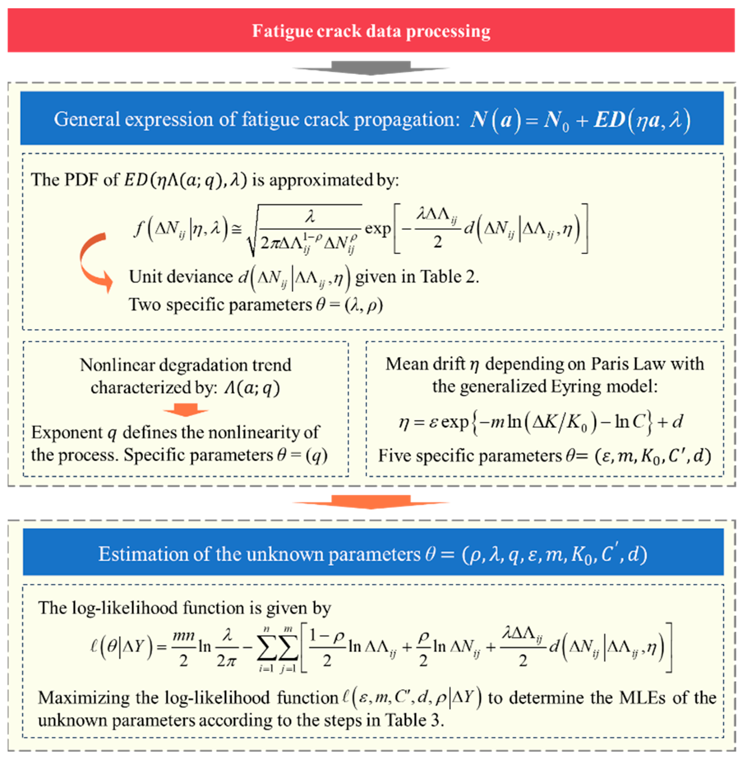
It has been considered that the best way to study the random propagation of fatigue cracks is to regard “the time required to reach a given crack length” as a stochastic process, and record it as [41]. Because the number of cycles is closely related to time, this paper regards “the number of cycles N required to reach a given crack length” as the research variable. Then, the variable from the Paris Law in Equation (3) can be seen to approximately follow the TEDP model, i.e., . Appendix A gives the specific proof for this.
Without loss of generality, the number of cycles required for crack growth to reach a given crack length follows the TEDP model. The physics-based TEDP model integrating the Paris Law is formulated by:
where ε and d are the compensation coefficients that need to be estimated. m represents the dependency of the crack growth rate on changes in the stress intensity factor, and C′ reflects the crack resistance and crack propagation susceptibility of the material.
According to the properties of TEDP, also has similar properties, as follows:
- (1)
- ;
- (2)
- has steady and independent increments;
- (3)
- The increment of cycle number follows the TED distribution.
Furthermore, as the degradation trajectory of crack propagation is nonlinear, a time scale function is introduced, which is usually determined by physical or empirical observation of degradation. A typical flexible form is that of the power function:
Correspondingly, the PDF of can be given by:
Then, the mean function and variance function of the physics-based TEDP model are respectively and . Additionally, the functional expression of is determined by the parameter ρ as follows:
where .
3.2. The PDF Based on Saddle-Joint Approximation
Although has an analytic form, it remains that in Equation (8) has no closed form, except for some special values. The saddle-point approximation method (SAM) can be used to obtain the PDF of the TEDP.
To find the saddle-point approximation of Equation (8), a unit deviation is defined as:
where D is the range of . Then, Equation (8) can be approximated by:
Then, the approximate expression of can be given by:
The detailed derivation process is presented in Appendix B.
However, as the specific expression of the unit deviation is still unknown, the calculation of Equation (12) remains difficult. Based on the formula of , as in Equation (9), the unit deviation function can be expressed in different forms under different values of ρ, as shown in Table 2.
3.3. Maximum Likelihood Estimation
Suppose that there are n samples, and that the crack length of the sample at the cycle number is , , . Let be the sampling number of the sample. The degradation increment of the two measured values is expressed as , and the increment of the length of the crack is expressed as . For the sample, and .
Considering that the samples are independent of each other, let be the joint probability density of the degradation of the sample, and be the joint probability density of the degradation of all samples.
where represents unknown parameters, and .
Therefore, the likelihood function of the unknown parameter θ of the physics-based TEDP model is given by:
Combining Equations (12) and (14), we can obtain the approximate expression of the log-likelihood function about the unknown parameter θ as follows:
The average degradation rate of crack propagation, η, is related to the crack propagation rate . That is, with respect to the material constants C′, and the stress intensity range , the average drift parameter η can be calculated by:
According to the above steps, the numerical expression of the likelihood function under the given parameter θ can be calculated. To find the MLE of θ, it is necessary to compare the likelihood function values under different values of θ to obtain its extreme value. Obviously, presetting a reasonable parameter range can greatly improve the efficiency of optimization. First, let the partial derivative of the Equation (15) be 0 for λ. Then, we have:
Substituting Equation (18) into Equation (15), we have a profile log-likelihood function, . Then, through setting the range of the unknown parameters, the optimization procedure of the likelihood function by the MLE method with respect to the unknown parameters is presented in Table 3.
To make the proposed parameter estimation procedure more intuitive, its schematic is shown in Figure 2.
4. Reliability Analysis
According to the meaning of degradation failure, the lifetime T of the product is generally defined as the time when the real performance degradation value reaches the failure threshold for the first time, that is, the first arrival time. In fatigue failure crack propagation, according to the theory of fracture mechanics, the failure point needs to be divided based on the critical stress value. The crack length threshold is related to , which is given by:
where .
We consider the time when the crack propagates to the critical value as the failure time, i.e.,
where is the number of cycles corresponding to the critical value of crack length. can be calculated by the following integral operation:
Based on the definition of lifetime, as in Equations (20) and (21), the reliability of a metal product under crack length can be expressed as:
Considering the computational complexity of the first arrival time of TEDP, the conditional CDF of cycle number N on parameter θ can be approximated using the Birnbaum–Saunders distribution [27,42], as follows:
where is the CDF of the standard normal distribution. Taking the derivative of yields the conditional PDF as follows:
The conditional reliability function of the metal product can be given by:
Therefore, the estimated p-percentile lifetime of the metal product can be computed by:
where is the p-percentile of the Gaussian distribution.
5. Case Study
5.1. Model Verification and Parameter Estimation
In this study, we used the statistical analysis results of crack propagation data from Virkler et al. [43]. The fatigue crack growth was investigated statistically. Sixty-eight repeated constant-amplitude crack propagation tests were carried out on 2024-T3 aluminum alloy, which was formed into a plate with a length of 558.8 mm, a width of 152.4 mm, and a thickness of 2.54 mm. Moreover, a central slit with a length of 2.54 mm and a width of 0.18 mm was machined as a stress lifting device. Figure 3 displays the number of load cycles in which the crack tip advanced by a predetermined increment a, from the initial crack length of 9 mm to the final length of 49.8 mm. Table 4 shows the experimental conditions. Further details can be found in [43].
After the data preprocessing, the proposed degradation model was applied for the reliability analysis. However, before using the physics-based TEDP model to analyze the reliability of the crack propagation process, had to be determined in advance. According to the curve trend, some deterministic models were selected through the definition of the Paris Law [17].
Because the dimensions in the length and width direction of the experiment were much larger than those in the thickness direction, and the load was located in the plane formed by the length and width direction, the problem met the conditions of the plane stress problem, and can thus be simplified as a plane stress problem. Therefore, Equation (4) can be modified to calculate in the following form:
where is a function that corrects for finite specimen width, and is the ratio of crack length to specimen width.
Equation (27) and the model mentioned above were used to estimate the unknown parameters. The specific parameter iteration process is shown in Figure 4. The estimation of all parameters reflected iterative convergence.
The parameter estimation results, based on the proposed maximum likelihood estimation method, are shown in Table 5. was calculated via linear regression, and C and η were calculated using Equation (6) and Equation (16), respectively.
5.2. Efficiency Comparison of Different Models
In order to illustrate the rationality and applicability of the proposed model, we used WP, GP, and IGP models to replace the TEDP model in the proposed physics-based TEDP model for comparison. An AIC criterion was used to evaluate the models’ performance. By combining the principles of information entropy and Kullback–Leibler distance, the AIC criterion encouraged the goodness of model fitting and avoided over-fitting as much as possible. Its specific definition was , where lnθ is the log-likelihood function and is the number of free parameters of the model. The comparative results are shown in Table 6.
As can be seen from Table 6, when ρ = 2.418, the log-likelihood function value of the physics-based TEDP model is the largest and the corresponding AIC value is the smallest, which indicates that it has high accuracy and low over-fitting risk in data fitting. Therefore, the TEDP model can be regarded as a suitable model for data compared with the WP, IGP, and GP models. This shows that the proposed model is more suitable for describing the degradation processes of fatigue crack propagation. By adjusting the value of the parameter ρ, this kind of TEDP model has better and wider applicability in degradation modeling.
The PDF and CDF curves of the product lifetime of the physics-based TEDP model and the other three models are shown in Figure 5 and Figure 6. It can be seen that the estimation result of the physics-based TEDP model was closer to that of the physics-based GP model. However, the physics-based WP and IGP models overestimated or underestimated the lifetime to varying degrees.
The proposed model was used to predict the crack growth, and the result is shown in Figure 7a. When the crack length was greater than 18 mm, the residual value was smaller, and the fitting effect of the model was better. The distribution of the residual errors of the prediction results is shown in Figure 7b. It can be seen that the residual value fluctuated around zero, and the model well explained and predicted the nonlinearity and randomness of the crack propagation process.
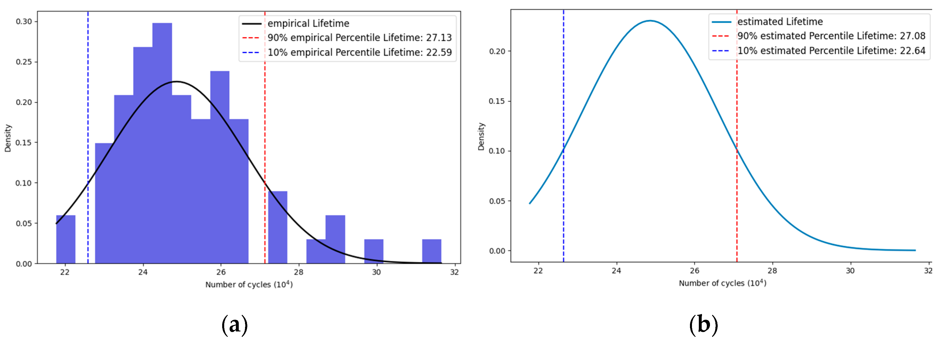
Given that Virkler’s dataset measured the number of cycles for a specified crack length, we redefined the p-percentile lifetime as defined by Equation (26) so that it was based on the number of cycles instead of crack length. We then compared the estimated results with the empirical lifetimes, and the result is shown in Figure 8. The graph presents a probability density function derived from empirical data on material fatigue, characterized by the number of cycles to failure. The alignment between the empirical lifetime and the modeled estimation signifies a robust correlation, indicating the model’s effectiveness in capturing the central tendency of the observed data.
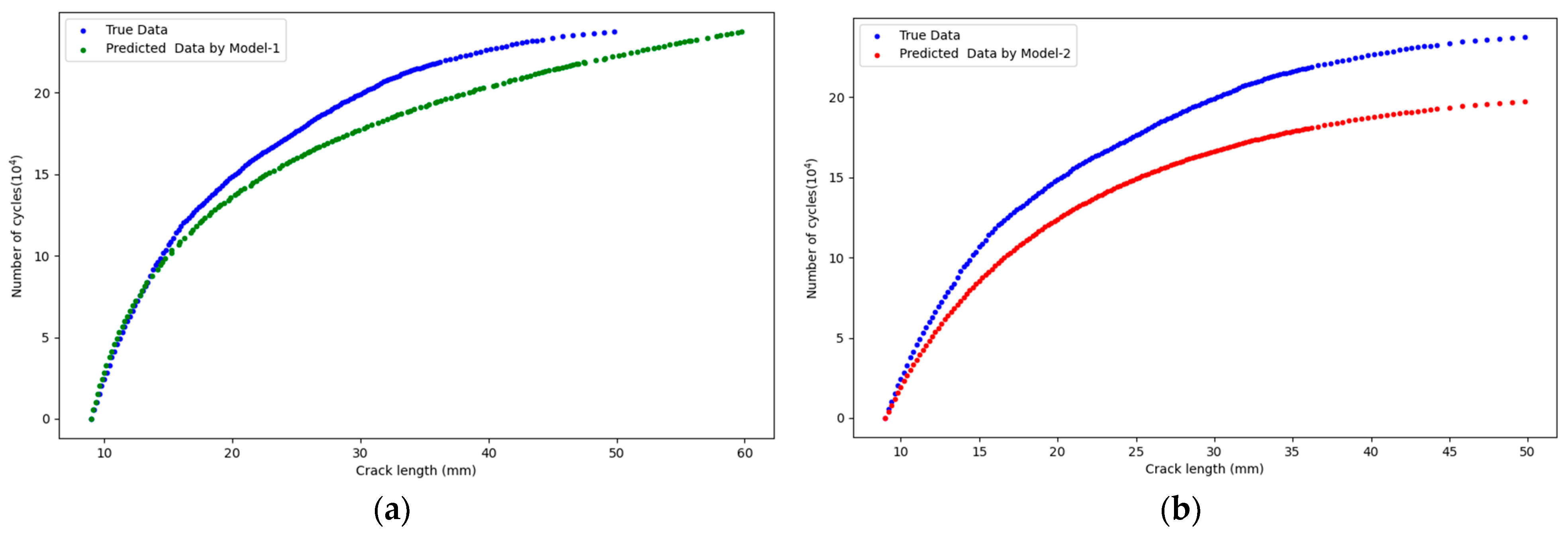
For the sake of further demonstrating the effectiveness and superiority of the proposed model, two other fatigue crack propagation models were employed as comparisons. The first one was a two-stage physics-based Wiener process model for the field vibration data of fatigue crack [36], which was denoted as Model-1. The other was a pure physical model based on the Paris Law from [44], which was denoted as Model-2. Because the parameters of Model-1 were related to the number of cycles (time scale) according to Paris Law, the time scale was not converted into crack length. The crack length was predicted directly under the corresponding number of cycles. The root mean square error (RMSE) between the predicted and true crack length values and the goodness-of-fit metric R2 of the model fitting were used as evaluation metrics to compare the performance of different models.
Table 7 shows the estimates of parameters and the evaluation metric values of different models. It can be seen that the R2 value of the proposed model was larger than that of Model-1, which indicates that the TEDP model fit the crack propagation paths much better than Model-1 when integrated with the Paris Law. This may be because the TEDP model was more flexible and accurate in describing complex nonlinear and random degradation paths through adjustment of the parameter ρ. Moreover, when comparing the RMSE values of the proposed model and Model-2, we found that the former again performed much better. This suggests clearly that the proposed model combines both the merits of physics models and stochastic processes, and can not only capture the fatigue crack growth paths accurately, but also represent the propagation uncertainty well. This indicates that both the physics information and crack data characteristics are fully utilized in the proposed model. Hence, the physics-based TEDP model can compensate for the deficiencies of the pure physical model in characterizing the randomness of crack growth, which is usually introduced by time-varying load conditions and the interference of environmental factors. Furthermore, Figure 9 also shows the prediction results of Model-1 and Model-2. Due to the accumulation of random deviations of WP, the predicted errors in Figure 9a become larger and larger as Model-2 is related to the estimated results of C and m. This model, while straightforward and widely used, tends to underperform in predicting crack growth in materials subjected to complex loading scenarios, and small deviations of C and m lead to larger errors in the predicted results. In short, we can see that physics-based TEDP model performed better than other models.
5.3. Discussion
We extensively analyzed the application and performance of the TEDP model in the context of fatigue crack propagation. The TEDP model demonstrated considerable flexibility and adaptability, effectively accommodating crack growth scenarios by adjusting parameters, particularly when describing complex, nonlinear, and stochastic degradation paths.
Despite its high adaptability and excellent statistical performance across multiple metrics, the effectiveness of the TEDP model is significantly constrained by the quality and type of the data it processes. The model presupposes that the degradation process is irreversible and monotonically increasing, and it handles increment data characterized as non-negative random variables. These assumptions may compromise the model’s accuracy in scenarios involving data with substantial fluctuations or directional changes, such as those encountered under periodic loading conditions or in complex stress environments. Consequently, in practical settings, especially where data characteristics do not align with these fundamental assumptions, the TEDP model may prove unsuitable or exhibit suboptimal performance. Notably, in specific scenarios, the TEDP model’s inherent flexibility and resilience allow it to adapt and include other models such as the Wiener process (WP) and Gaussian process (GP), enabling it to handle a broader range of data types.
6. Conclusions
In view of the uncertainty in the process of metal fatigue crack propagation, a Tweedie exponential dispersion model based on proportional Paris Law was established, and parameter estimation was conducted using the maximum likelihood estimation algorithm based on saddle-point approximation. The model was applied to Virkler fatigue test data to demonstrate its effectiveness. The results showed that the proposed model can fit cracks well. Compared with previous studies on fatigue crack propagation, which have generally relied on a single random process or a pure physics model, the proposed model exhibited several significant improvements as follows:
- (1)
- Enhanced flexibility and adaptability. Adjusting the parameters of the TEDP model through the Paris Law can diversify the flexibility and adaptability of the proposed model, which is of great significance in reflecting the actual crack propagation process given its nonlinear and random characteristics. Both the physical and data-based information types relating to fatigue crack propagation are fully utilized.
- (2)
- Mathematical transparency and traceability. The model is further strengthened by integrating the MLE estimation of saddle-point approximation techniques. These methods together endow the physics-based TEDP model with extraordinary mathematical transparency and traceability. The effectiveness of the framework is verified by case study.
- (3)
- Quantitative analysis of lifetime and reliability. The analytic expressions of the distributions of lifetime and product reliability are derived, which can not only provide predictions of fatigue lifetime, but also quantify the uncertainty of crack propagation.
Although the proposed model in this paper includes a comprehensive quantitative uncertainty method, it can be further improved by comprehensively considering environmental conditions and other factors. In future, we can use various real data from different industries in order to verify the model and apply it in predictive maintenance systems, with the aim of providing a reliable tool for industry professionals to use in the effective prediction and management of the life cycle of structural components.
Author Contributions
Conceptualization, L.Y. and Z.C.; software, L.Y.; validation, Z.W., Z.C. and E.P. All authors have read and agreed to the published version of the manuscript.
Funding
This work is supported in part by the Natural Science Foundation of Shanghai under Grant 23ZR1428100, and in part by the National Key Research and Development Program of China under Grant 2022YFF0605700.
Data Availability Statement
The data presented in this study are openly available in FigShare in ref. [43].
Acknowledgments
The authors would like to thank the editor and anonymous referees for their careful work and remarkable comments, which helped to improve this manuscript substantially.
Conflicts of Interest
The authors declare no conflict of interest.
Appendix A
It is known that
The number of crack propagation cycles can be expressed by:
where and indicate the observation times, and a and are independent of each other.
Let the characteristic function of be . The definitions of the moment generating function and the characteristic function are respectively expressed by:
By the nature of independence, the characteristic function of the crack extension length a is:
In order to prove is the characteristic function of Tweedie exponential random variables, we need to meet two conditions:
- (1)
- is 1 at t = 0. This condition is the basic requirement of the characteristic function (that is, the characteristic function is 1 at the origin).
- (2)
- is an analytic function on the complex plane. This condition guarantees the existence and uniqueness of the characteristic function.
Firstly, we verify that is 1 at t = 0, i.e.,
Next, we need to prove is an analytic function on the complex plane. To prove this, we need to prove the existence and continuity of the derivative of .
Suppose that the derivative of exists and is continuous, which is denoted as . According to the nature of the derivative, the derivative of the characteristic function of the crack propagation length a can be expressed as
Note that, the derivative of each exists and is continuous. Therefore, the derivative of also exists and is continuous.
Therefore, we can draw the conclusion that the crack propagation length obeys the Tweedie exponential dispersion process.
- (1)
- .
- (2)
- has steady and independent increments.
- (3)
- Each increment obeys the Tweedie exponential distribution, as in Equation (1).
According to the properties of TEDP, the mean function and variance function of the above stochastic process are and , respectively.
Appendix B
According to the above descriptions, the PDF of the increments is given by:
Then, its characteristic function is given by:
When is completely integrable, the PDF of can be expressed by Fourier inversion theorem as follows:
Since the integrand function is analytic, the integral region of Equation (A12) can be shifted from to . Then, the unit deviation in Equation (10) can be obtained.
Expanding based on the Taylor series at yields the following expression:
For the TEDP model, the variance function can be expressed as follows:
Substituting Equations (A13) and (A14) into Equation (A10), the PDF can be derived.
References
- Wang, R.; Xu, J.; Zhang, W.; Gao, J.; Li, Y.; Chen, F. Reliability analysis of complex electromechanical systems: State of the art, challenges, and prospects. Qual. Reliab. Eng. Int. 2022, 38, 3935–3969. [Google Scholar] [CrossRef]
- Campbell, F. Elements of Metallurgy and Engineering Alloys; ASM International: Almere, The Netherlands, 2008. [Google Scholar]
- Ellis, B.; Heyns, P.S.; Schmidt, S. A hybrid framework for remaining useful life estimation of turbomachine rotor blades. Mech. Syst. Signal Process. 2022, 170, 108805. [Google Scholar] [CrossRef]
- Khan, A.; Azad, M.M.; Sohail, M.; Kim, H.S. A Review of Physics-based Models in Prognostics and Health Management of Laminated Composite Structures. Int. J. Precis. Eng. Manuf. Technol. 2023, 10, 1615–1635. [Google Scholar] [CrossRef]
- Pimenov, D.Y.; da Silva, L.R.; Ercetin, A.; Der, O.; Mikolajczyk, T.; Giasin, K. State-of-the-art review of applications of image processing techniques for tool condition monitoring on conventional machining processes. Int. J. Adv. Manuf. Technol. 2024, 130, 57–85. [Google Scholar] [CrossRef]
- Serin, G.; Sener, B.; Ozbayoglu, A.M.; Unver, H.O. Review of tool condition monitoring in machining and opportunities for deep learning. Int. J. Adv. Manuf. Technol. 2020, 109, 953–974. [Google Scholar] [CrossRef]
- Pugno, N.; Ciavarella, M.; Cornetti, P.; Carpinteri, A. A generalized Paris’ law for fatigue crack growth. J. Mech. Phys. Solids 2006, 54, 1333–1349. [Google Scholar] [CrossRef]
- Baral, T.; Afshari, S.S.; Liang, X. Residual life prediction of aluminum alloy plates under cyclic loading using an integrated prognosis method. Trans. Can. Soc. Mech. Eng. 2023, 47, 467–474. [Google Scholar] [CrossRef]
- Yang, L.; Zhang, J.; Guo, Y.; Wang, P. A Bayesian-based Reliability Estimation Approach for Corrosion Fatigue Crack Growth Utilizing the Random Walk. Qual. Reliab. Eng. Int. 2016, 32, 2519–2535. [Google Scholar] [CrossRef]
- Nejad, R.M.; Liu, Z.; Ma, W.; Berto, F. Fatigue reliability assessment of a pearlitic Grade 900A rail steel subjected to multiple cracks. Eng. Fail. Anal. 2021, 128, 105625. [Google Scholar] [CrossRef]
- Kuncham, E.; Sen, S.; Kumar, P.; Pathak, H. An online model-based fatigue life prediction approach using extended Kalman filter. Theor. Appl. Fract. Mech. 2021, 117, 103143. [Google Scholar] [CrossRef]
- Gao, Y.; Li, L.; Zhang, Y. Modeling Crack Propagation in Bituminous Binders under a Rotational Shear Fatigue Load using Pseudo J-Integral Paris’ Law. Transp. Res. Rec. J. Transp. Res. Board 2020, 2674, 94–103. [Google Scholar] [CrossRef]
- An, D.; Kim, N.H.; Choi, J.-H. Practical options for selecting data-driven or physics-based prognostics algorithms with reviews. Reliab. Eng. Syst. Saf. 2015, 133, 223–236. [Google Scholar] [CrossRef]
- Wang, Y.; Huang, Y.; Liao, W. Degradation analysis on trend gamma process. Qual. Reliab. Eng. Int. 2022, 38, 941–956. [Google Scholar] [CrossRef]
- Meeker, W.; Escobar, L.; Lu, C. Accelerated degradation tests: Modeling and analysis. Technometrics 1998, 40, 89–99. [Google Scholar] [CrossRef]
- Yuan, X.-X. Pandey A nonlinear mixed-effects model for degradation data obtained from in-service inspections. Reliab. Eng. Syst. Saf. 2009, 94, 509–519. [Google Scholar] [CrossRef]
- Lawless, J.; Crowder, M. Covariates and random effects in a gamma process model with application to degradation and failure. Lifetime Data Anal. 2004, 10, 213–227. [Google Scholar] [CrossRef] [PubMed]
- Ye, Z.-S.; Xie, M.; Tang, L.-C.; Chen, N. Semiparametric Estimation of Gamma Processes for Deteriorating Products. Technometrics 2014, 56, 504–513. [Google Scholar] [CrossRef]
- Peng, W.; Li, Y.-F.; Yang, Y.-J.; Zhu, S.-P.; Huang, H.-Z. Bivariate analysis of incomplete degradation observations based on inverse Gaussian processes and copulas. IEEE Trans. Reliab. 2016, 65, 624–639. [Google Scholar] [CrossRef]
- Chen, L.; Huang, T.; Zhou, H. Stochastic Modeling of Metal Fatigue Crack Growth Using Proportional Paris Law and Inverse Gaussian Process. Eng. Mech. 2021, 38, 238–247. [Google Scholar]
- Wang, X. Wiener processes with random effects for degradation data. J. Multivar. Anal. 2010, 101, 340–351. [Google Scholar] [CrossRef]
- Peng, C.-Y. Inverse Gaussian processes with random effects and explanatory variables for degradation data. Technometrics 2015, 57, 100–111. [Google Scholar] [CrossRef]
- Tweedie, M. An index which distinguishes between some important exponential families. In Proceedings of the Indian Statistical Institute Golden Jubilee International Conference, Indian Statistical Institute, Calcutta, India, 17–20 December 1984; pp. 579–604. [Google Scholar]
- Sen, A.; Jorgensen, B. The Theory of Dispersion Models. Technometrics 1999, 41, 177. [Google Scholar] [CrossRef]
- Yan, W.; Zhang, S.; Liu, W.; Yu, Y. Objective Bayesian Estimation for Tweedie Exponential Dispersion Process. Mathematics 2021, 9, 2740. [Google Scholar] [CrossRef]
- Tseng, S.; Lee, I. Optimum Allocation Rule for Accelerated Degradation Tests with a Class of Exponential-Dispersion Degradation Models. Technometrics 2016, 58, 244–254. [Google Scholar] [CrossRef]
- Hong, L.; Ye, Z. When is acceleration unnecessary in a degradation test? Stat. Sin. 2017, 27, 1461–1483. [Google Scholar]
- Duan, F.; Wang, G. Exponential-dispersion degradation process models with random effects and covariates. IEEE Trans. Reliab. 2018, 67, 1128–1142. [Google Scholar] [CrossRef]
- Chen, Z.; Pan, E.; Xia, T.; Li, Y. Optimal degradation-based burn-in policy using Tweedie exponential-dispersion process model with measurement errors. Reliab. Eng. Syst. Saf. 2019, 195, 106748. [Google Scholar] [CrossRef]
- Chen, Z.; Xia, T.; Li, Y.; Pan, E. Tweedie exponential dispersion processes for degradation modeling, prognostic, and accelerated degradation test planning. IEEE Trans. Reliab. 2019, 69, 887–902. [Google Scholar] [CrossRef]
- Chen, Z.; Xia, T.; Li, Y.; Pan, E. Random-effect models for degradation analysis based on nonlinear Tweedie exponential-dispersion processes. IEEE Trans. Reliab. 2021, 71, 47–62. [Google Scholar] [CrossRef]
- Duan, F.; Wang, G. Generalized exponential-dispersion process model for degradation analysis under nonlinear condition. Qual. Reliab. Eng. Int. 2021, 38, 957–970. [Google Scholar] [CrossRef]
- Yan, W.; Riahi, H.; Benzarti, K.; Chlela, R.; Curtil, L.; Bigaud, D. Durability and reliability estimation of flax fiber reinforced composites using tweedie exponential dispersion degradation process. Math. Probl. Eng. 2021, 2021, 6629637. [Google Scholar] [CrossRef]
- Zhou, S.; Xu, A. Exponential dispersion process for degradation analysis. IEEE Trans. Reliab. 2019, 68, 398–409. [Google Scholar] [CrossRef]
- Ding, Y.; Zhu, R.; Peng, W.; Xie, M. Degradation analysis with nonlinear exponential-dispersion process: Bayesian offline and online perspectives. Qual. Reliab. Eng. Int. 2022, 38, 3844–3866. [Google Scholar] [CrossRef]
- Yan, B.; Ma, X.; Huang, G.; Zhao, Y. Two-stage physics-based Wiener process models for online RUL prediction in field vibration data. Mech. Syst. Signal Process. 2020, 152, 107378. [Google Scholar] [CrossRef]
- Jorgensen, B. Exponential Dispersion Models. J. R. Stat. Soc. Ser. B Stat. Methodol. 1987, 49, 127–145. [Google Scholar]
- Paris, P.; Erdogan, F. A Critical Analysis of Crack Propagation Laws. J. Basic Eng. 1963, 85, 528–533. [Google Scholar] [CrossRef]
- Cavallini, M. A statistical analysis of fatigue crack growth in a 2091 Al Cu Li alloy. Int. J. Fatigue 1995, 17, 135–139. [Google Scholar] [CrossRef]
- Bergner, F.; Zouhar, G. A new approach to the correlation between the coefficient and the exponent in the power law equation of fatigue crack growth. Int. J. Fatigue 2000, 22, 229–239. [Google Scholar] [CrossRef]
- Guida, M.; Penta, F. A gamma process model for the analysis of fatigue crack growth data. Eng. Fract. Mech. 2015, 142, 21–49. [Google Scholar] [CrossRef]
- Virkler, D.A.; Hillberry, B.M.; Goel, P.K. The statistical nature of fatigue crack propagation. J. Eng. Mater. Technol. 1979, 101, 148–153. [Google Scholar] [CrossRef]
- Birnbaum, Z.; Saunders, S. A New Family of Life Distributions. J. Appl. Probab. 1969, 6, 319–327. [Google Scholar] [CrossRef]
- Ditlevsen, O.; Olesen, R. Statistical analysis of the virkler data on fatigue crack growth. Eng. Fract. Mech. 1986, 25, 177–195. [Google Scholar] [CrossRef]
Figure 1.
Fatigue crack growth rate curve. Note: The corresponding point at log((1 – R)Kc) is defined as the failure point.
Figure 1.
Fatigue crack growth rate curve. Note: The corresponding point at log((1 – R)Kc) is defined as the failure point.
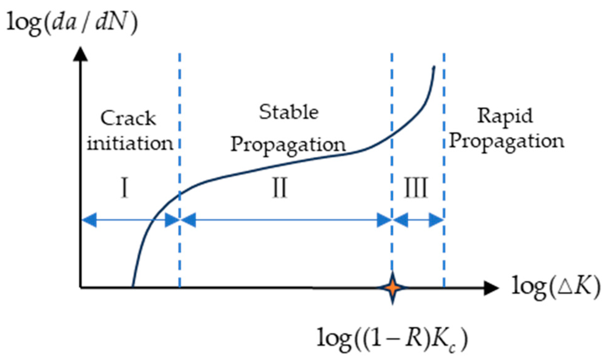
Figure 2.
The parameter estimation process for the physics-based TEDP model.

Figure 3.
Test specimen and Virkler dataset. (a) Test specimen; (b) 68 crack growth curves observed by Virkler et al. [43]
Figure 3.
Test specimen and Virkler dataset. (a) Test specimen; (b) 68 crack growth curves observed by Virkler et al. [43]
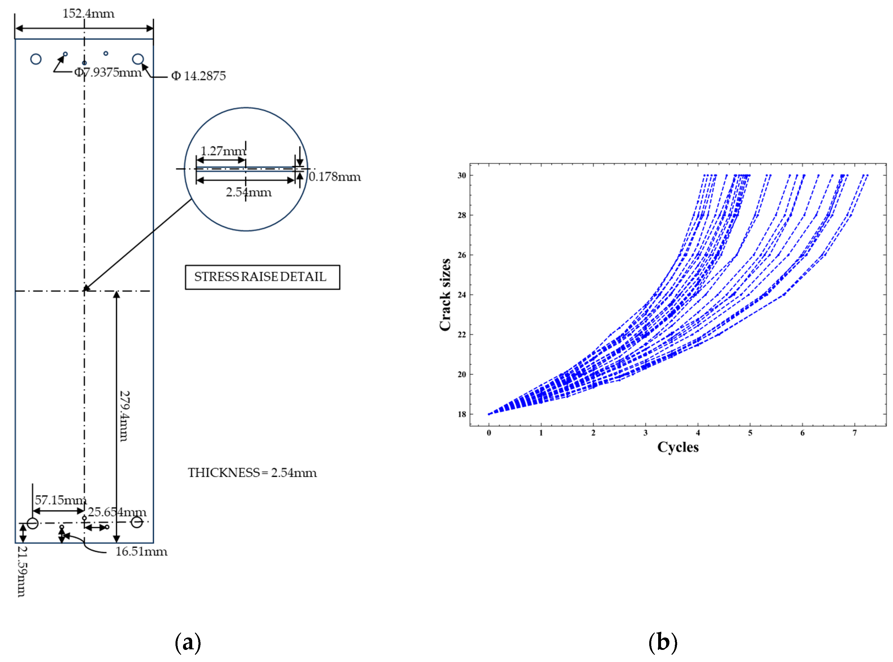
Figure 4.
Parameter iteration processes. (a) Iteration of parameter λ; (b) Iteration of parameter ρ; (c) Iteration of parameter ε; (d) Iteration of parameter m; (e) Iteration of parameter d; (f) Iteration of parameter q; (g) Iteration of parameter b (Represents the reciprocal of C).
Figure 4.
Parameter iteration processes. (a) Iteration of parameter λ; (b) Iteration of parameter ρ; (c) Iteration of parameter ε; (d) Iteration of parameter m; (e) Iteration of parameter d; (f) Iteration of parameter q; (g) Iteration of parameter b (Represents the reciprocal of C).
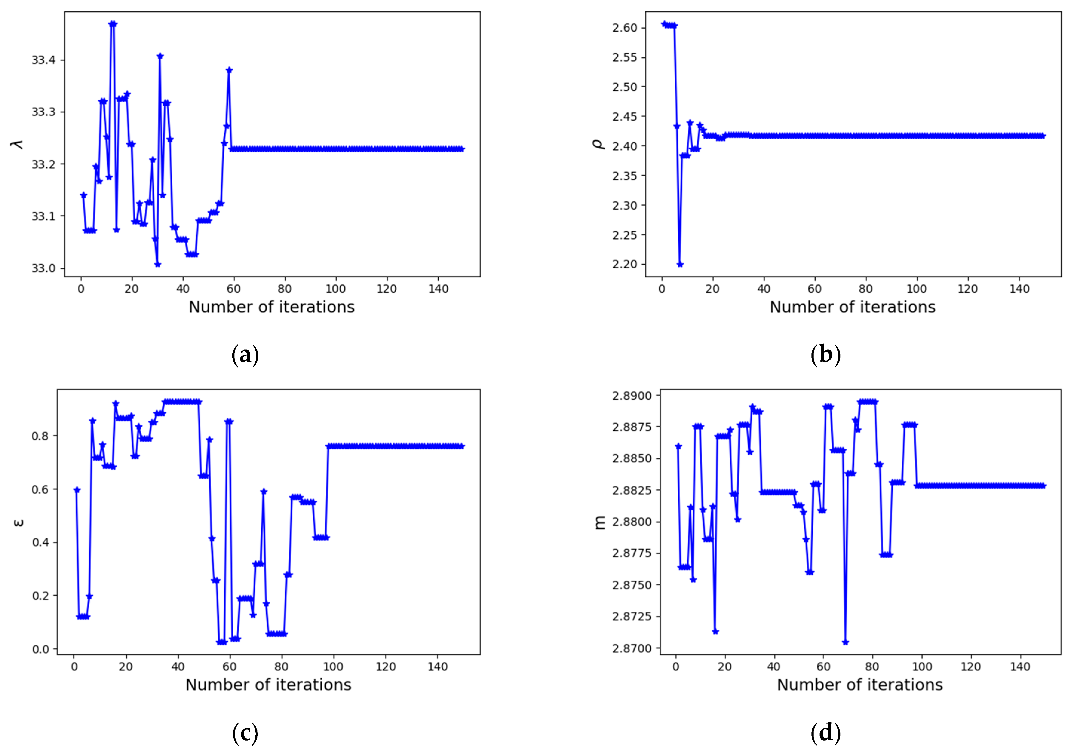
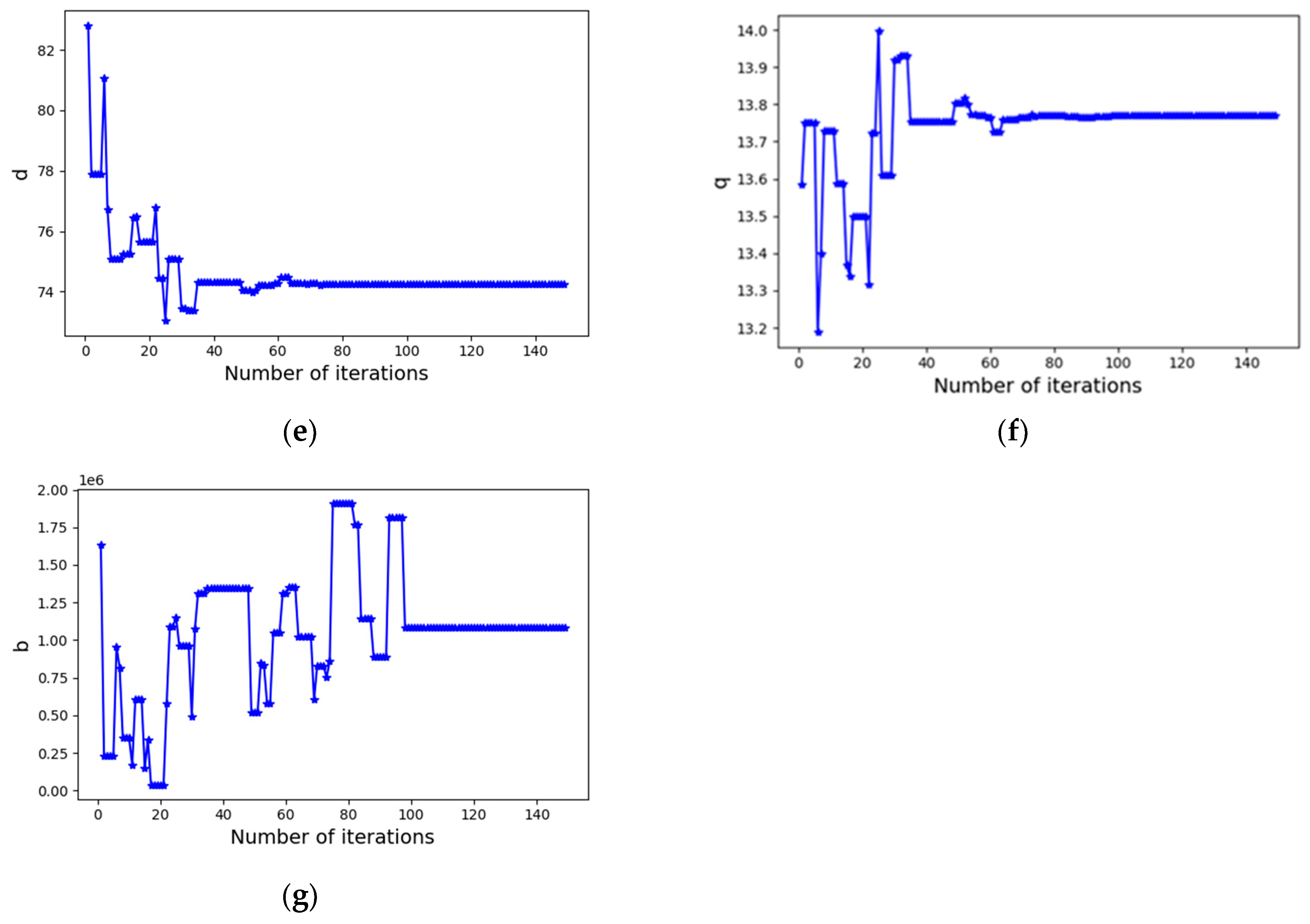
Figure 5.
Comparisons of the estimated PDFs of the lifetime based on different models.
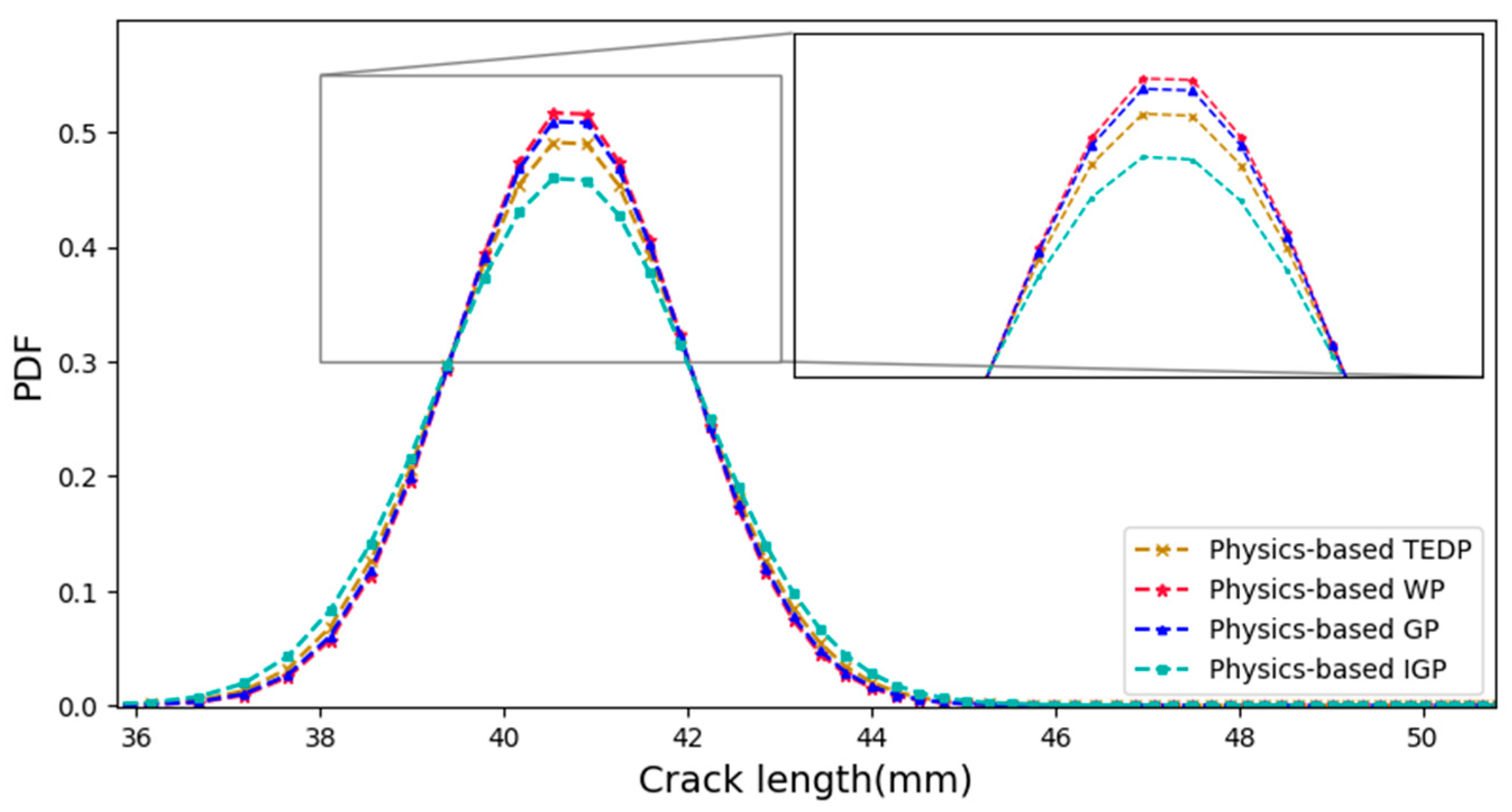
Figure 6.
Comparisons of the estimated CDFs of the lifetime based on different models.
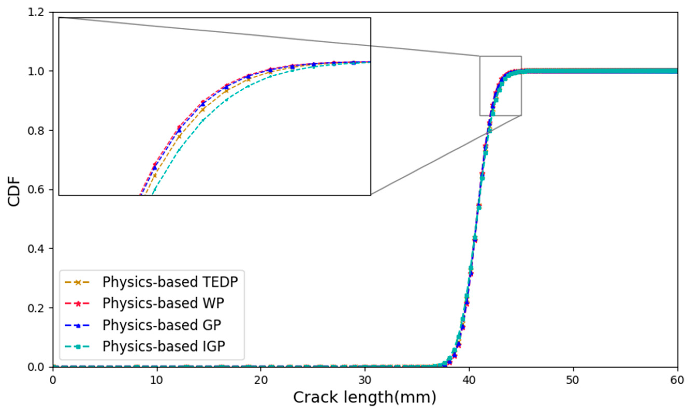
Figure 7.
Prediction results of the proposed model. (a) Predictions of cycle number N(a); (b) The residual errors of predictions.
Figure 7.
Prediction results of the proposed model. (a) Predictions of cycle number N(a); (b) The residual errors of predictions.

Figure 8.
Prediction p-percentile lifetime of the proposed model. (a) Empirical p-percentile lifetime; (b) Prediction p-percentile lifetime of the proposed model.
Figure 8.
Prediction p-percentile lifetime of the proposed model. (a) Empirical p-percentile lifetime; (b) Prediction p-percentile lifetime of the proposed model.

Figure 9.
The prediction results of Model-1 and Model 2. (a) Estimation of crack length a by Model-1; (b) Prediction of cycle number N(a) by Model-2.
Figure 9.
The prediction results of Model-1 and Model 2. (a) Estimation of crack length a by Model-1; (b) Prediction of cycle number N(a) by Model-2.

Table 1.
Tweedie exponential dispersion stochastic process.
| The Distribution Form | ρ | The Distribution Form | ρ |
|---|---|---|---|
| Extremely stable | Gamma | ||
| Gaussian | Positive stable | ||
| Poisson | Inverse Gaussian | ||
| Compound Poisson | Positive stable |
Table 2.
Formulae of the unit deviation under different ρ.
| ρ | |
| ρ = 0 | |
| ρ = 1 | |
| ρ = 2 | |
Table 3.
Optimization procedure of the unknown model parameters via MLE.
| Step 1 | Set the initial value and the range of . |
| Step 2 | Set the iterative step size h. |
| Step 3 | Maximize the corresponding profile likelihood function. |
| Step 4 | Repeat Step 3, and get a likelihood function set |
| Step 5 | Select the largest value to obtain the MLE, |
Table 4.
Experimental conditions and other related parameters.
| Loading Mode | R | |
|---|---|---|
| Compound Poisson | 0.2 | 24.14 Mpa |
Table 5.
Parameter estimation results of the proposed model.
| η | λ | ρ | q | ||||
|---|---|---|---|---|---|---|---|
| ε | m | C | d | 33.228 | 2.418 | 11.697 | 0.203 |
| 0.837 | 2.881 | 7.863 × 10⁻⁵ | 74.234 | ||||
| 1.2873 | |||||||
Table 6.
Parameter estimation results of the compared model.
| Model | Estimates | lnθ | AIC | ||
|---|---|---|---|---|---|
| η | λ | ρ | |||
| Physics-based TEDP | 1.287 | 33.228 | 2.418 | 14,760.407 | −29024.8 |
| Physics-based WP | 1.287 | 20.039 | 0 | 12,712.825 | −25413.6 |
| Physics-based GP | 1.287 | 32.222 | 2 | 14,691.802 | −28996.6 |
| Physics-based IGP | 1.287 | 33.607 | 3 | 14,614.402 | −28357.3 |
Table 7.
Comparison of results between different fatigue crack propagation models.
| Model | Estimates of Parameters | RMSE | R2 |
|---|---|---|---|
| The proposed model | η = 1.287, λ = 33.228 ρ = 2.418, C = 7.863 × 10⁻⁵ m = 2.881 | 0.8919 | 0.9757 |
| Model-1 | η = 0.140, σB2 = 2.057 × 10⁻¹⁸ μa = −3.65 × 10⁻²⁰, σα2 = 1.877 | - | 0.7319 |
| Model-2 | C = 8.03 × 10⁻⁵ m = 2.872 | 5.1338 | - |
Disclaimer/Publisher’s Note: The statements, opinions and data contained in all publications are solely those of the individual author(s) and contributor(s) and not of MDPI and/or the editor(s). MDPI and/or the editor(s) disclaim responsibility for any injury to people or property resulting from any ideas, methods, instructions or products referred to in the content. |
© 2024 by the authors. Licensee MDPI, Basel, Switzerland. This article is an open access article distributed under the terms and conditions of the Creative Commons Attribution (CC BY) license (https://creativecommons.org/licenses/by/4.0/).
Share and Cite
MDPI and ACS Style
Yang, L.; Wang, Z.; Chen, Z.; Pan, E. A Physics-Based Tweedie Exponential Dispersion Process Model for Metal Fatigue Crack Propagation and Prognostics. Processes 2024, 12, 849. https://doi.org/10.3390/pr12050849
AMA Style
Yang L, Wang Z, Chen Z, Pan E. A Physics-Based Tweedie Exponential Dispersion Process Model for Metal Fatigue Crack Propagation and Prognostics. Processes. 2024; 12(5):849. https://doi.org/10.3390/pr12050849
Chicago/Turabian StyleYang, Lin, Zirong Wang, Zhen Chen, and Ershun Pan. 2024. "A Physics-Based Tweedie Exponential Dispersion Process Model for Metal Fatigue Crack Propagation and Prognostics" Processes 12, no. 5: 849. https://doi.org/10.3390/pr12050849
Note that from the first issue of 2016, this journal uses article numbers instead of page numbers. See further details here.