
Real-Time Optimization under Uncertainty Applied to a Gas Lifted Well Network


Abstract
:
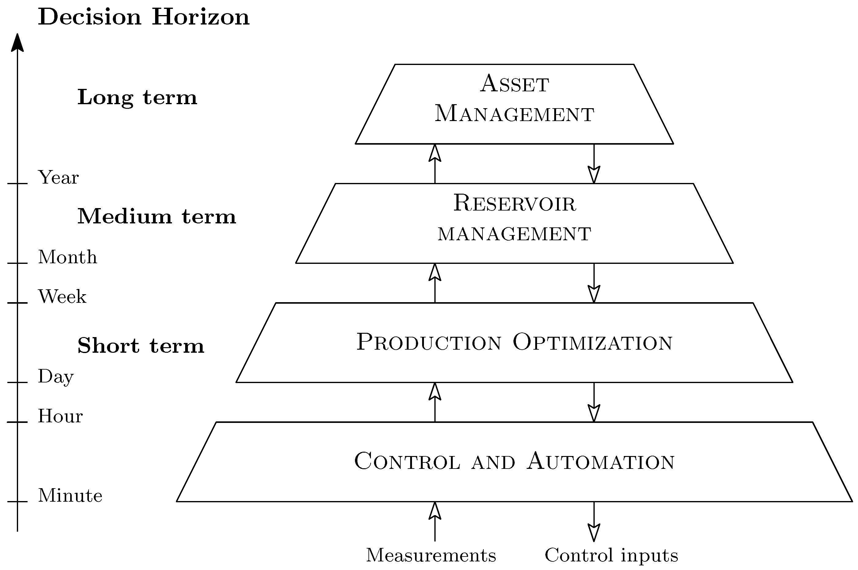
1. Introduction
- Model uncertainty—in which the underlying structure of the model is uncertain due to lack of knowledge or model simplification.
- Parametric uncertainty—where the parameters are outdated or have insufficient excitation to be determined accurately.
- Measurement error—any model to some extent relies on measured data which have a certain degree of uncertainty.
- The calculated optimal solution, which is thought to be feasible, might actually violate the problem constraints and therefore be infeasible when implemented.
- When the optimal solution is feasible, the solution may be far from the actual optimal value, and hence is suboptimal.
2. Previous Work
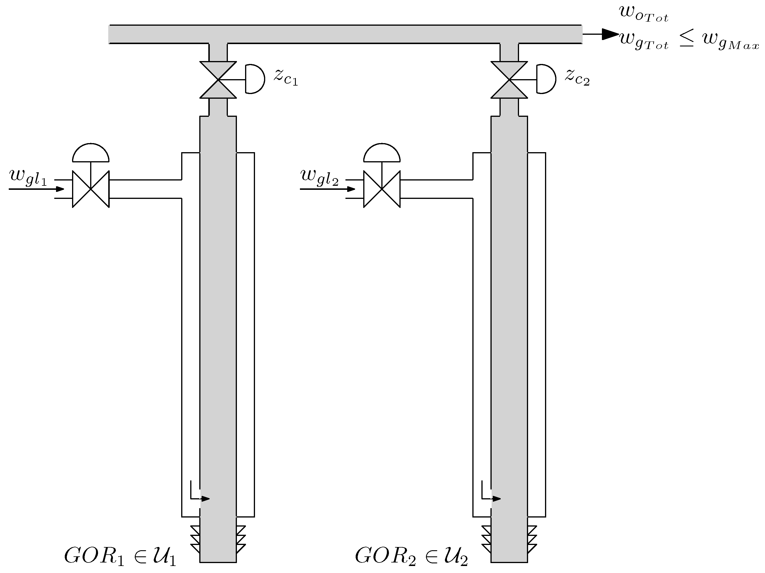
3. Process Description
3.1. Modelling of Gas Lifted Wells
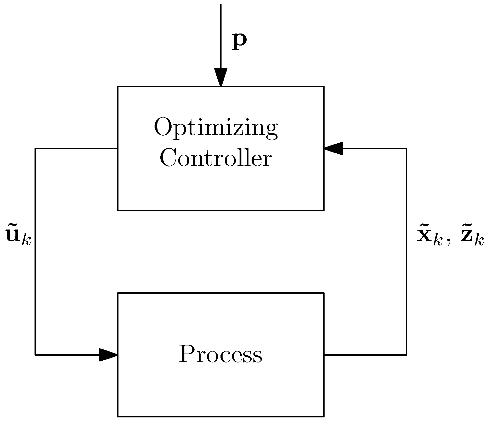
4. Optimization under Uncertainty
4.1. Scenario Optimization
5. Simulation Results
6. Discussion
7. Materials and Methods
8. Conclusions
Acknowledgments
Author Contributions
Conflicts of Interest
Abbreviations
| RTO | Real-Time Optimization |
| DAE | Differential Algebraic Equations |
| ODE | Ordinary Differential Equations |
| NLP | Nonlinear Programming Problem |
| NMPC | Nonlinear Model Predictive Control |
| GOR | Gas–Oil Ratio |
| PI | Productivity Index |
| DPO | Daily Production Optimization |
References
- Foss, B.A.; Jensen, J.P. Performance analysis for closed-loop reservoir management. SPE J. 2011, 16, 183–190. [Google Scholar] [CrossRef]
- Elgsæter, S.M. Modeling and Optimizing the Offshore Production of Oil and Gas under Uncertainty. Ph.D. Thesis, Norwegian University of Science and Technology (NTNU), Trondheim, Norway, 2008. [Google Scholar]
- Ben-Tal, A.; Nemirovski, A. Robust solutions of linear programming problems contaminated with uncertain data. Math. Program. 2000, 88, 411–424. [Google Scholar] [CrossRef]
- Bieker, H.P.; Slupphaug, O.; Johansen, T.A. Real time production optimization of offshore oil and gas production systems: A technology survey. In Intelligent Energy Conference and Exhibition; Society of Petroleum Engineers: Amsterdam, The Netherlands, 2006. [Google Scholar]
- Scokaert, P.; Mayne, D. Min-max feedback model predictive control for constrained linear systems. IEEE Trans. Autom. Control 1998, 43, 1136–1142. [Google Scholar] [CrossRef]
- Lucia, S.; Finkler, T.; Engell, S. Multi-stage nonlinear model predictive control applied to a semi-batch polymerization reactor under uncertainty. J. Proc. Control 2013, 23, 1306–1319. [Google Scholar] [CrossRef]
- Wang, P.; Litvak, M.; Aziz, K. Optimization of production operations in petroleum fields. In SPE Annual Technical Conference and Exhibition; Society of Petroleum Engineers: San Antonio, TX, USA, 2002. [Google Scholar]
- Gunnerud, V.; Foss, B. Oil production optimization—A piecewise linear model, solved with two decomposition strategies. Comput. Chem. Eng. 2010, 34, 1803–1812. [Google Scholar] [CrossRef]
- Camponogara, E.; Nakashima, P.H. Solving a gas-lift optimization problem by dynamic programming. Eur. J. Oper. Res. 2006, 174, 1220–1246. [Google Scholar] [CrossRef]
- Camponogara, E.; Nakashima, P. Optimizing gas-lift production of oil wells: piecewise linear formulation and computational analysis. IIE Trans. 2006, 38, 173–182. [Google Scholar] [CrossRef]
- Codas, A.; Camponogara, E. Mixed-integer linear optimization for optimal lift-gas allocation with well-separator routing. Eur. J. Oper. Res. 2012, 217, 222–231. [Google Scholar] [CrossRef]
- Codas, A.; Jahanshahi, E.; Foss, B. A two-layer structure for stabilization and optimization of an oil gathering network. IFAC-PapersOnLine 2016, 49, 931–936. [Google Scholar] [CrossRef]
- Elgsæter, S.M.; Slupphaug, O.; Johansen, T.A. A structured approach to optimizing offshore oil and gas production with uncertain models. Comput. Chem. Eng. 2010, 34, 163–176. [Google Scholar] [CrossRef]
- Bieker, H.P.; Slupphaug, O.; Johansen, T.A. Well management under uncertain gas or water oil ratios. In Digital Energy Conference and Exhibition; Society of Petroleum Engineers: Houston, TX, USA, 2007. [Google Scholar]
- Hanssen, K.G.; Foss, B. Production Optimization under Uncertainty-Applied to Petroleum Production. IFAC-PapersOnLine 2015, 48, 217–222. [Google Scholar] [CrossRef]
- Hülse, E.O.; Camponogara, E. Robust formulations for production optimization of satellite oil wells. Eng. Optim. 2016, 1–18. [Google Scholar] [CrossRef]
- Sharma, R.; Glemmestad, B. On generalized reduced gradient method with multi-start and self-optimizing control structure for gas lift allocation optimization. J. Proc. Control 2013, 23, 1129–1140. [Google Scholar] [CrossRef]
- Eikrem, G.O.; Imsland, L.; Foss, B. Stabilization of gas-lifted wells based on state estimation. 2004. Available online: http://folk.ntnu.no/bjarnean/pubs/conference/conf-75.pdf?id=ansatte/Foss_Bjarne/pubs/conference/conf-75.pdf (accessed on 14 December 2016).
- Peixoto, A.J.; Pereira-Dias, D.; Xaud, A.F.; Secchi, A.R. Modelling and Extremum Seeking Control of Gas Lifted Oil Wells. IFAC-PapersOnLine 2015, 48, 21–26. [Google Scholar] [CrossRef]
- Jahanshahi, E. Control Solutions for Multiphase Flow: Linear and nonlinear approaches to anti-slug control. Ph.D. Thesis, Norwegian University of Science and Technology (NTNU), Trondheim, Norway, 2013. [Google Scholar]
- Jahanshahi, E.; Skogestad, S. Simplified Dynamic Models for Control of Riser Slugging in Offshore Oil Production. Oil Gas Facil. 2014, 3, 80–88. [Google Scholar] [CrossRef]
- Alstad, V. Studies on Selection of Controlled Variables. Ph.D. Thesis, Norwegian University of Science and Technology (NTNU), Trondheim, Norway, 2005. [Google Scholar]
- Krishnamoorthy, D.; Bergheim, E.M.; Pavlov, A.; Fredriksen, M.; Fjalestad, K. Modelling and Robustness Analysis of Model Predictive Control for Electrical Submersible Pump Lifted Heavy Oil Wells. IFAC-PapersOnLine 2016, 49, 544–549. [Google Scholar] [CrossRef]
- Eikrem, G.O.; Aamo, O.M.; Foss, B.A. On instability in gas lift wells and schemes for stabilization by automatic control. SPE Prod. Oper. 2008, 23, 268–279. [Google Scholar] [CrossRef]
- Golan, M.; Whitson, C.H. Well Performance, 2nd ed.; Tapir: Trondheim, Norway, 1995. [Google Scholar]
- Biegler, L.T. Nonlinear Programming: Concepts, Algorithms, and Applications to Chemical Processes; SIAM: Philadelphia, PA, USA, 2010; Volume 10. [Google Scholar]
- Soyster, A.L. Technical note—Convex programming with set-inclusive constraints and applications to inexact linear programming. Oper. Res. 1973, 21, 1154–1157. [Google Scholar] [CrossRef]
- Skogestad, S.; Postlethwaite, I. Multivariable Feedback Control: Analysis and Design, 2nd ed.; Wiley: New York, NY, USA, 2007. [Google Scholar]
- Andersson, J. A General-Purpose Software Framework for Dynamic Optimization. Ph.D. Thesis, Arenberg Doctoral School, KU Leuven, Department of Electrical Engineering (ESAT/SCD) and Optimization in Engineering Center, Kasteelpark Arenberg, Belgium, 2013. [Google Scholar]
- Wächter, A.; Biegler, L.T. On the implementation of an interior-point filter line-search algorithm for large-scale nonlinear programming. Math. Program. 2006, 106, 25–57. [Google Scholar] [CrossRef]
- Lucia, S.; Paulen, R. Robust nonlinear model predictive control with reduction of uncertainty via robust optimal experiment design. IFAC Proc. Vol. 2014, 47, 1904–1909. [Google Scholar] [CrossRef]


| Parameter | Units | Well 1 | Well 2 | Comment |
|---|---|---|---|---|
| [m] | 1500 | 1500 | Length of well | |
| [m] | 1000 | 1000 | Height of well | |
| [m] | 0.121 | 0.121 | Diameter of well | |
| [m] | 500 | 500 | Length of well below injection | |
| [m] | 100 | 100 | Height of well below injection | |
| [m] | 0.121 | 0.121 | Diameter of well below injection | |
| [m] | 1500 | 1500 | Length of annulus | |
| [m] | 1000 | 1000 | Height of annulus | |
| [m] | 0.189 | 0.189 | Diameter of annulus | |
| [kg/m] | 900 | 800 | Density of Oil | |
| [m] | 1 | 1 | Injection valve characteristic | |
| [m] | 1 | 1 | Production valve characteristic | |
| [bar] | 20 | 20 | Manifold pressure | |
| [bar] | 150 | 155 | Reservoir pressure | |
| [kg·s·bar] | 2.2 | 2.2 | Productivity index | |
| [C] | 28 | 28 | Annulus temperature | |
| [C] | 32 | 32 | Well tubing temperature | |
| [g] | 20 | 20 | Molecular weight of gas | |
| [kg/kg] | 0.1 ± 0.1 | 0.15 ± 0.01 | Gas–Oil ratio |
| Well | Nominal | Worst Case | Scenario-Based | |||
|---|---|---|---|---|---|---|
| GOR well 1 | 0.1 | 0.2 | 0.05 | 0.1 | 0.15 | 0.2 |
| GOR well 2 | 0.15 | 0.16 | 0.145 | 0.15 | 0.155 | 0.16 |
| Optimization | True GOR | True Optimum | Computed Optimum | Potential | Obtained | Loss | |||
|---|---|---|---|---|---|---|---|---|---|
| Well 1 | Well 2 | Well 1 | Well 2 | Well 1 | Well 2 | Tot Oil | Tot Oil | ||
| [kg/kg] | [kg/kg] | [kg/s] | [kg/s] | [kg/s] | [kg/s] | [kg/s] | [kg/s] | [kg/s] | |
| Nominal case | 0.05 | 0.145 | 3.337 | 1.5117 | 2.663 | 1.518 | 31.879 | 31.7 | 0.179 |
| 0.1 | 0.15 | 2.563 | 1.429 | 2.563 | 1.429 | 31.879 | 31.879 | 0 | |
| 0.15 | 0.155 | 1.788 | 1.348 | infeasible | infeasible | 31.879 | infeasible | - | |
| 0.2 | 0.16 | 1.014 | 1.266 | infeasible | infeasible | 31.879 | infeasible | - | |
| Worst case | 0.05 | 0.145 | 3.337 | 1.5117 | 1.324 | 1.32 | 31.879 | 30.69 | 1.189 |
| 0.1 | 0.15 | 2.563 | 1.429 | 1.318 | 1.329 | 31.879 | 31.33 | 0.549 | |
| 0.15 | 0.155 | 1.788 | 1.348 | 1.235 | 1.317 | 31.879 | 31.69 | 0.189 | |
| 0.2 | 0.16 | 1.014 | 1.266 | 1.014 | 1.266 | 31.879 | 31.879 | 0 | |
| Scenario tree | 0.05 | 0.145 | 3.337 | 1.5117 | 2.048 | 0.7046 | 31.879 | 31.12 | 0.759 |
| 0.1 | 0.15 | 2.563 | 1.429 | 2.036 | 0.6904 | 31.879 | 31.49 | 0.389 | |
| 0.15 | 0.155 | 1.788 | 1.348 | 2.038 | 0.5616 | 31.879 | 31.67 | 0.209 | |
| 0.2 | 0.16 | 1.014 | 1.266 | 2.007 | 0.2697 | 31.879 | 31.68 | 0.199 | |
© 2016 by the authors; licensee MDPI, Basel, Switzerland. This article is an open access article distributed under the terms and conditions of the Creative Commons Attribution (CC-BY) license (http://creativecommons.org/licenses/by/4.0/).
Share and Cite
Krishnamoorthy, D.; Foss, B.; Skogestad, S. Real-Time Optimization under Uncertainty Applied to a Gas Lifted Well Network. Processes 2016, 4, 52. https://doi.org/10.3390/pr4040052
Krishnamoorthy D, Foss B, Skogestad S. Real-Time Optimization under Uncertainty Applied to a Gas Lifted Well Network. Processes. 2016; 4(4):52. https://doi.org/10.3390/pr4040052
Chicago/Turabian StyleKrishnamoorthy, Dinesh, Bjarne Foss, and Sigurd Skogestad. 2016. "Real-Time Optimization under Uncertainty Applied to a Gas Lifted Well Network" Processes 4, no. 4: 52. https://doi.org/10.3390/pr4040052