2D Plane Strain Consolidation Process of Unsaturated Soil with Vertical Impeded Drainage Boundaries

Abstract

The consolidation process of soil stratum is a common issue in geotechnical engineering. In this paper, the two-dimensional (2D) plane strain consolidation process of unsaturated soil was studied by incorporating vertical impeded drainage boundaries. The eigenfunction expansion and Laplace transform techniques were adopted to transform the partial differential equations for both the air and water phases into two ordinary equations, which can be easily solved. Then, the semi-analytical solutions for the excess pore-pressures and the soil layer settlement were derived in the Laplace domain. The final results in the time domain could be computed by performing the numerical inversion of Laplace transform. Furthermore, two comparisons were presented to verify the accuracy of the proposed semi-analytical solutions. It was found that the semi-analytical solution agreed well with the finite difference solution and the previous analytical solution from the literature. Finally, the 2D plane strain consolidation process of unsaturated soil under different drainage efficiencies of the vertical boundaries was illustrated, and the influences of the air-water permeability ratio, the anisotropic permeability ratio and the spacing-depth ratio were investigated.

1. Introduction

The consolidation process of soil stratum is a common issue in geotechnical engineering and it has captured a great deal of attention in the geotechnical community. In the mid-1920s, Terzaghi [1] put forward the classical one-dimensional (1D) consolidation process for saturated soil, after which some researchers derived the solutions to 1D consolidation process for saturated soil subjected to different loading and boundary conditions [2,3,4,5]. With the problem raised in practical engineering, much attention has been attracted to the consolidation process of unsaturated soil since the 1960s. Scott [6] discussed the consolidation process of unsaturated soil with occluded air bubbles, and Barden [7,8] presented a study of the compacted unsaturated soil. Furthermore, Fredlund and Hasan [9] proposed a 1D consolidation theory by driving two partial differential equations (PDEs) to describe the dissipation processes of excess pore-air and -water pressures. Dakshanamurthy and Fredlund [10] extended this theory to two-dimensional (2D) plane strain consolidation process by referring the concept of 2D heat diffusion. These theories have been widely accepted in geotechnical engineering and have inspired numerous research projects on the consolidation process of unsaturated soil [11,12,13,14,15].

In order to ensure that analytical solutions were available, most of the previous studies treated the top and bottom drainage boundaries of the soil layer as fully drained or undrained [16]. However, these boundaries are generally partially drained (i.e., impeded drainage) in most practical consolidation processes. For example, a sand cushion covered on the top surface of the soil layer, which is commonly used to facilitate the drainage, will become partially drained when its drainage capacity is not effective. The underlying layer will exhibit impeded drainage characteristic when its void ratio is relatively small. In order to describe the partially drained effect, Gray [17] defined an impeded drainage boundary using the third type boundary, which can also realize the fully drained and undrained boundaries (i.e., the first and second type boundaries) by changing the values of the boundary parameters. Base on this boundary, a number of solutions have been proposed to solve the 1D consolidation process of saturated soil [16,17,18,19,20] and that of unsaturated soil [21,22,23]. These solutions help to understand the impeding effect (i.e., drainage efficiency) of the covered sand cushion and underlying layer on the 1D consolidation process. However, in the study of the 2D plane strain consolidation processes, particularly for unsaturated soil, there appears no solution incorporating the impeded drainage boundaries. The objective of this paper was to develop a general solution to the 2D plane strain consolidation process of unsaturated soil under such impeded drainage boundaries, that is, the top surface and bottom base of the soil layer were considered to be partially drained.

Based on the consolidation equations proposed by Dakshanamurthy and Fredlund [10], this paper attempted to derive semi-analytical solutions to the 2D plane strain consolidation process of unsaturated soil by incorporating the vertical impeded drainage boundaries. To obtain the final solutions, the eigenfunction expansion and Laplace transform techniques were used to transform PDEs of both air and water phases into two ordinary equations. Then, the solutions for the excess pore-pressures and the soil layer settlement were derived in the Laplace domain, and the final results can be computed by performing the numerical inversion of Laplace transform. Furthermore, two comparisons against the finite difference solution and the previous analytical solution were made to verify the accuracy of the proposed solution. Finally, some computations were conducted to study the 2D plane strain consolidation process of unsaturated soil incorporating vertical impeded drainage boundaries.

2. Mathematical Model

2.1. Governing Equations

In geotechnical practice, vertical drain assisted with preloading is one of the most commonly used techniques to improve the soft soil. The vertical drain can facilitate the consolidation process by providing a shorter drainage path in the horizontal direction. Figure 1 illustrates a referential consolidation system of a homogeneous unsaturated soil layer with two installed vertical drains, in which the vertical boundaries are presumed to be impeded drainage to the air and water phases. This system extends the problem considered by Ho et al. [14,15].

The thickness of the soil layer was $H$, and the internal spacing of vertical drains was $L$. In the soil layer, the coefficients of permeability with respect to the air and water in the x-direction were $k_{\mathrm{ax}}$ and $k_{\mathrm{wx}}$, and those in z-direction were $k_{\mathrm{az}}$ and $k_{\mathrm{wz}}$, respectively. On and under the soil layer were two impedance layers, and their thicknesses were $H_0$ and $H_1$, respectively. These two impedance layers were considered to be permeable in z-direction only. In the upper impedance layer, the coefficients of permeability with respect to the air and water were $k_{\mathrm{a}0}$ and $k_{\mathrm{w}0}$, respectively; those in the down impedance layer were $k_{\mathrm{a}1}$ and $k_{\mathrm{w}1}$, respectively. The external load $q_0$ was assumed to be constant and uniformly distributed on the top of the upper impedance layer.

For a constant external load instantaneously applied, the governing equations for 2D plane strain consolidation process of unsaturated soil can be expressed as follows [10,14,15]:

$$\frac{\partial u_{\mathrm{a}}}{\partial t}+C_{\mathrm{a}}\frac{\partial u_{\mathrm{w}}}{\partial t}+c_{\mathrm{vx}}^{\mathrm{a}}\frac{{\partial }^2{u}_{\mathrm{a}}}{\partial x^2}+c_{\mathrm{vz}}^{\mathrm{a}}\frac{{\partial }^2{u}_a}{\partial z^2}=0$$

(1a)

$$\frac{\partial u_{\mathrm{w}}}{\partial t}+C_{\mathrm{w}}\frac{\partial u_{\mathrm{a}}}{\partial t}+c_{\mathrm{vx}}^{\mathrm{w}}\frac{{\partial }^2{u}_{\mathrm{w}}}{\partial x^2}+c_{\mathrm{vz}}^{\mathrm{w}}\frac{{\partial }^2{u}_{\mathrm{w}}}{\partial z^2}=0$$

(1b)

where $u_{\mathrm{a}}$ and $u_{\mathrm{w}}$ are the excess pore-air and -water pressures, respectively (kPa); $C_{\mathrm{a}}$ and $C_{\mathrm{w}}$ are the interactive constants associated with the air and water phases, respectively; $c_{\mathrm{vx}}^{\mathrm{a}}$ and $c_{\mathrm{vx}}^{\mathrm{w}}$ are the consolidation coefficients with respect to the air and water phases in x-direction, respectively (m²/s); and $c_{\mathrm{vz}}^{\mathrm{a}}$ and $c_{\mathrm{vz}}^{\mathrm{w}}$ are the consolidation coefficients with respect to the air and water phases in z-direction, respectively (m²/s). These consolidation parameters can be expressed as follows:

$$C_{\mathrm{a}}={\left[\left(\frac{2m_1^{\mathrm{a}}}{m_2^{\mathrm{a}}}-1\right)-\frac{n\left(1-S_{\mathrm{r}}\right)}{m_2^{\mathrm{a}}\left(u_{\mathrm{a}}^0+u_{\mathrm{atm}}\right)}\right]}^{-1}$$

(2a)

$$c_{\mathrm{vx}}^{\mathrm{a}}=\frac{k_{\mathrm{ax}}\mathrm{R}\mathsf{\Theta }}{\mathrm{gM}}{\left[m_2^{\mathrm{a}}\left(u_{\mathrm{a}}^0+u_{\mathrm{atm}}\right)\left(\frac{2m_1^{\mathrm{a}}}{m_2^{\mathrm{a}}}-1\right)-n\left(1-S_r\right)\right]}^{-1}$$

(2b)

$$c_{\mathrm{vz}}^{\mathrm{a}}=\frac{k_{\mathrm{az}}\mathrm{R}\mathsf{\Theta }}{\mathrm{gM}}{\left[m_2^{\mathrm{a}}\left(u_{\mathrm{a}}^0+u_{\mathrm{atm}}\right)\left(\frac{2m_1^{\mathrm{a}}}{m_2^{\mathrm{a}}}-1\right)-n\left(1-S_r\right)\right]}^{-1}$$

(2c)

$$C_{\mathrm{w}}=\frac{2m_1^{\mathrm{w}}}{m_2^{\mathrm{w}}}-1$$

(2d)

$$c_{\mathrm{vx}}^{\mathrm{w}}=\frac{k_{\mathrm{wx}}}{m_2^{\mathrm{w}}{\gamma }_{\mathrm{w}}}$$

(2e)

$$c_{\mathrm{vz}}^{\mathrm{w}}=\frac{k_{\mathrm{wz}}}{m_2^{\mathrm{w}}{\gamma }_{\mathrm{w}}}$$

(2f)

where $m_1^{\mathrm{a}}$ and $m_1^{\mathrm{w}}$ are the coefficients of air and water volume change with respect to the change of the net normal stress, respectively (kPa⁻¹); $m_2^{\mathrm{a}}$ and $m_2^{\mathrm{w}}$ are the coefficients of air and water volume change with respect to the change of suction, respectively (kPa⁻¹); $n$ is the soil porosity; $S_r$ is the degree of saturation; $u_{\mathrm{atm}}$ is the atmospheric pressure (kPa); $\mathsf{\Theta }$ is the absolute temperature (K); $\mathrm{R}$ is the universal air constant (8.314 J·mol⁻¹·K⁻¹); $g$ is the gravitational acceleration (9.8 m/s²); $M$ is the molecular mass of air phase (0.029 kg/mol); and ${\gamma }_{\mathrm{w}}$ is the unite weight of water (9.8 kN/m³).

2.2. Initial and Boundary Conditions

It was assumed that immediately after the application of the external load, the initial excess pore-air and -water pressures were distributed uniformly throughout the entire stratum. That is:

$$\begin{array}{cc}{u}_{\mathrm{a}}\left(x,z,0\right)=u_{\mathrm{a}}^0,& u_{\mathrm{w}}\left(x,z,0\right)=u_{\mathrm{w}}^0\end{array}$$

(3)

where $u_{\mathrm{a}}^0$ and $u_{\mathrm{w}}^0$ are the values of the initial excess pore-air and -water pressures, respectively.

The horizontal (i.e., left and right) boundaries, which were defined by two vertical drains, were all considered to permeable to the air and water phases. That is:

$$u_{\mathrm{a}}\left(0,z,t\right)=u_{\mathrm{a}}\left(L,z,t\right)=u_{\mathrm{w}}\left(0,z,t\right)=u_{\mathrm{w}}\left(L,z,t\right)=0$$

(4)

The vertical (i.e., top and bottom) boundaries, which were separately defined by sand cushion and underlying layer, were considered to be partially permeable to the air and water phases. That is:

$$\begin{array}{cc}\frac{\partial u_{\mathrm{a}}\left(x,0,t\right)}{\partial z}-\frac{R_{\mathrm{ta}}}{H}{u}_{\mathrm{a}}\left(x,0,t\right)=0,& \frac{\partial u_{\mathrm{w}}\left(x,0,t\right)}{\partial z}-\frac{R_{\mathrm{tw}}}{H}{u}_{\mathrm{w}}\left(x,0,t\right)=0\end{array}$$

(5a)

$$\begin{array}{cc}\frac{\partial u_{\mathrm{a}}\left(x,H,t\right)}{\partial z}+\frac{R_{\mathrm{ba}}}{H}{u}_{\mathrm{a}}\left(x,H,t\right)=0,& \frac{\partial u_{\mathrm{w}}\left(x,H,t\right)}{\partial z}+\frac{R_{\mathrm{bw}}}{H}{u}_{\mathrm{w}}\left(x,H,t\right)=0\end{array}$$

(5b)

where $R_{\mathrm{ta}}=k_{\mathrm{az}0}H/k_{\mathrm{az}}{H}_0$ and $R_{\mathrm{tw}}=k_{\mathrm{wz}0}H/k_{\mathrm{wz}}{H}_0$, and they are two dimensionless characteristic factors describing the drainage efficiency of the top surface to the air and water phases, respectively; $R_{\mathrm{ba}}=k_{\mathrm{az}1}H/k_{\mathrm{az}}{H}_1$ and $R_{\mathrm{bw}}=k_{\mathrm{wz}1}H/k_{\mathrm{wz}}{H}_1$, and they are two dimensionless characteristic factors describing the drainage efficiency of the bottom base to the air and water phases, respectively. When it is assumed that $R_{\mathrm{ta}}=R_{\mathrm{tw}}=\infty$ and $R_{\mathrm{ba}}=R_{\mathrm{bw}}=\infty$, the vertical boundaries are double drainage (i.e., top-base drainage [14,15]). For this scenario, both the top and bottom surfaces were permeable to the air and water phases. When it is assumed that $R_{\mathrm{ta}}=R_{\mathrm{tw}}=\infty$ and $R_{\mathrm{ba}}=R_{\mathrm{bw}}=0$, the vertical boundaries are single drainage (i.e., top drainage [14,15]). For this scenario, the top surface was permeable to the air and water phase, whereas the bottom base was impermeable to the air and water phases.

3. Solution Formulation and Verification

In general, unsaturated soil is complex in natural property and engineering behavior due to the lack of homogeneity, the complicate texture, the interaction of multiphase and the nonlinear feature. In order to handle the mathematical derivation easily, some essential assumptions were made along with those used in the 2D plane strain consolidation theory of unsaturated soil [10,14,15].

The prominent assumptions are listed as follows:

(1)

The soil stratum was considered to be homogeneous;

(2)

The soil particle and pore water were incompressible;

(3)

The flows of the air and water phases were continuous and independent, and simultaneously, they only took place in two directions (i.e., the x- and z-directions);

(4)

During the consolidation process, the deformation occurring was small and the coefficients of the volume change for the soil stratum remained constant;

(5)

The consolidation parameters with respect to the air phase (i.e., $C_{\mathrm{a}}$, $c_{\mathrm{vx}}^{\mathrm{a}}$ and $c_{\mathrm{vz}}^{\mathrm{a}}$) and those with respect to the water phase (i.e., $C_{\mathrm{w}}$, $c_{\mathrm{vx}}^{\mathrm{w}}$ and $c_{\mathrm{vz}}^{\mathrm{w}}$) remained constant during the consolidation process; and

(6)

The effect of air diffusing through water, air dissolving in water, the movement of water vapor and temperature change were ignored.

The above assumptions were not completely accurate for all cases. The consolidation parameters may change because of the variations in the soil properties, such as the permeability coefficients, degree of saturation and porosity, and moreover, the modulus for the soil and the water phase were nonlinear. However, in order to obtain the solution to the consolidation equations of unsaturated soil more easily, it may be acceptable to assume that these soil properties remain constant during the transient process for a small stress increment. Moreover, these constant properties have been commonly adopted to study the consolidation process of unsaturated soil in some existing analytical and semi-analytical methods proposed by Lo et al. [11,14,15], Zhou et al. [12], Shan et al. [13] and Wang et al. [21,22,23].

3.1. Solution Formulation

Equations (1a) and (1b) can be rewritten as follows:

$$\frac{\partial u_{\mathrm{a}}}{\partial t}=\frac{1}{1-C_{\mathrm{a}}{C}_{\mathrm{w}}}\left[C_{\mathrm{a}}{c}_{\mathrm{vz}}^{\mathrm{w}}\left({\kappa }_{\mathrm{w}}\frac{{\partial }^2{u}_{\mathrm{w}}}{\partial x^2}+\frac{{\partial }^2{u}_{\mathrm{w}}}{\partial z^2}\right)-c_{\mathrm{vz}}^{\mathrm{a}}\left({\kappa }_{\mathrm{a}}\frac{{\partial }^2{u}_{\mathrm{a}}}{\partial x^2}+\frac{{\partial }^2{u}_a}{\partial z^2}\right)\right]$$

(6a)

$$\frac{\partial u_{\mathrm{w}}}{\partial t}=\frac{1}{1-C_{\mathrm{a}}{C}_{\mathrm{w}}}\left[C_{\mathrm{w}}{c}_{\mathrm{vz}}^{\mathrm{a}}\left({\kappa }_{\mathrm{a}}\frac{{\partial }^2{u}_{\mathrm{a}}}{\partial x^2}+\frac{{\partial }^2{u}_a}{\partial z^2}\right)-c_{\mathrm{vz}}^{\mathrm{w}}\left({\kappa }_{\mathrm{w}}\frac{{\partial }^2{u}_{\mathrm{w}}}{\partial x^2}+\frac{{\partial }^2{u}_{\mathrm{w}}}{\partial z^2}\right)\right]$$

(6b)

where ${\kappa }_{\mathrm{a}}=k_{\mathrm{ax}}/k_{\mathrm{az}}$ and ${\kappa }_{\mathrm{w}}=k_{\mathrm{wx}}/k_{\mathrm{wz}}$, and they are two anisotropic permeability ratios of the air and water phases, respectively. Through defining two alternative variables ${\varphi }_1$ and ${\varphi }_2$, Equations (6a) and (6b) can be transformed into:

$$\frac{\partial {\varphi }_1}{\partial t}=Q_1\left(\frac{{\partial }^2{\varphi }_1}{\partial z^2}+{\rho }_{11}\frac{{\partial }^2{\varphi }_1}{\partial x^2}+{\rho }_{21}\frac{{\partial }^2{\varphi }_2}{\partial x^2}\right)$$

(7a)

$$\frac{\partial {\varphi }_2}{\partial t}=Q_2\left(\frac{{\partial }^2{\varphi }_2}{\partial z^2}+{\rho }_{12}\frac{{\partial }^2{\varphi }_1}{\partial x^2}+{\rho }_{22}\frac{{\partial }^2{\varphi }_2}{\partial x^2}\right)$$

(7b)

where:

$${\varphi }_1=u_{\mathrm{a}}+c_{21}{u}_{\mathrm{w}},{\varphi }_2=c_{12}{u}_{\mathrm{a}}+u_{\mathrm{w}}$$

(8)

$${\rho }_{11}=\frac{{\kappa }_{\mathrm{w}}{c}_{12}{c}_{21}-{\kappa }_{\mathrm{a}}}{c_{12}{c}_{21}-1},{\rho }_{21}=\frac{{\kappa }_{\mathrm{a}}{c}_{21}-{\kappa }_{\mathrm{w}}{c}_{21}}{c_{12}{c}_{21}-1},{\rho }_{12}=\frac{{\kappa }_{\mathrm{w}}{c}_{12}-{\kappa }_{\mathrm{a}}{c}_{12}}{c_{12}{c}_{21}-1},{\rho }_{22}=\frac{{\kappa }_{\mathrm{a}}{c}_{12}{c}_{21}-{\kappa }_{\mathrm{w}}}{c_{12}{c}_{21}-1}$$

(9)

The details of derivation process and meanings of $c_{21}$ and $c_{12}$ can be found in Appendix A. It is noteworthy that Equations (7a) and (7b) will become two uncoupled PDEs when ${\kappa }_{\mathrm{a}}={\kappa }_{\mathrm{w}}$, and their solutions can be obtained more easily than coupled ones. However, for the sake of generality the solutions are derived below for the coupled case of Equations (7a) and (7b).

Substituting Equation (4) into Equation (8) gives:

$${\varphi }_1\left(0,z,t\right)={\varphi }_1\left(L,z,t\right)={\varphi }_2\left(0,z,t\right)={\varphi }_2\left(L,z,t\right)=0$$

(10)

These boundary conditions above are homogeneous; thus, the general solutions of Equations (7a) and (7b) can be expressed as follows:

$${\varphi }_1\left(x,z,t\right)={\displaystyle \sum _{i=1}^{\infty }{\phi }_1^i\left(z,t\right)\cdot \sin \left({\mu }_{i}x\right)}$$

(11a)

$${\varphi }_2\left(x,z,t\right)={\displaystyle \sum _{i=1}^{\infty }{\phi }_2^i\left(z,t\right)\cdot \sin \left({\mu }_{i}x\right)}$$

(11b)

where ${\phi }_1^i$ and ${\phi }_2^i$ are the generalized Fourier coefficients of ${\varphi }_1$ and ${\varphi }_2$ with respect to $x$, respectively; and ${\mu }_i=i\pi /L$.

Substituting Equations (11a) and (11a) into Equations (7a) and (7b) result in:

$$\frac{\partial {\phi }_1^i}{\partial t}=Q_1\left(\frac{{\partial }^2{\phi }_1^i}{\partial z^2}-{\rho }_{11}{\mu }_i^2{\phi }_1^i-{\rho }_{21}{\mu }_i^2{\phi }_2^i\right)$$

(12a)

$$\frac{\partial {\phi }_2^i}{\partial t}=Q_2\left(\frac{{\partial }^2{\phi }_2^i}{\partial z^2}-{\rho }_{12}{\mu }_i^2{\phi }_1^i-{\rho }_{22}{\mu }_i^2{\phi }_2^i\right)$$

(12b)

Implementing the Laplace transforms on Equations (12a) and (12b), and rearranging gives:

$$Q_1\frac{d^2{\tilde{\phi }}_1^i}{d{z}^2}=\left(s+Q_1{\rho }_{11}{\mu }_i^2\right){\tilde{\phi }}_1^i+Q_1{\rho }_{21}{\mu }_i^2{\tilde{\phi }}_2^i-{\phi }_1^{i0}$$

(13a)

$$Q_2\frac{{\partial }^2{\tilde{\phi }}_2^i}{\partial z^2}=Q_2{\rho }_{12}{\mu }_i^2{\tilde{\phi }}_1^i+\left(s+Q_2{\rho }_{22}{\mu }_i^2\right){\tilde{\phi }}_2^i-{\phi }_2^{i0}$$

(13b)

where:

$${\phi }_1^{i0}={\vartheta }_i\left(u_{\mathrm{a}}^0+c_{21}{u}_{\mathrm{w}}^0\right),{\phi }_2^{i0}={\vartheta }_i\left(c_{12}{u}_{\mathrm{a}}^0+u_{\mathrm{w}}^0\right)$$

(14)

and ${\vartheta }_i=2\left[1-{\left(-1\right)}^i\right]/\left({\mu }_{i}L\right)$.

The solutions of Equations (13a) and (13b) subjected to the impeded drainage boundaries are:

$${\tilde{\phi }}_1^i={\chi }_1{e}^{{\lambda }_{1}z}+{\chi }_2{e}^{-{\lambda }_{1}z}+{\psi }_2\left({\chi }_3{e}^{{\lambda }_{2}z}+{\chi }_4{e}^{-{\lambda }_{2}z}\right)+{\chi }_5$$

(15a)

$${\tilde{\phi }}_2^i={\psi }_1\left({\chi }_1{e}^{{\lambda }_{1}z}+{\chi }_2{e}^{-{\lambda }_{1}z}\right)+{\chi }_3{e}^{{\lambda }_{2}z}+{\chi }_4{e}^{-{\lambda }_{2}z}+{\chi }_6$$

(15b)

The derivation details and meanings of ${\chi }_1$~${\chi }_6$, ${\lambda }_1$, ${\lambda }_2$, ${\psi }_1$ and ${\psi }_2$ can be found in Appendix B.

Implementing the Laplace transform on Equation (A22) gives:

$${\tilde{u}}_{\mathrm{a}}={\displaystyle \sum _{i=1}^{\infty }\left(\frac{{\tilde{\phi }}_1^i-c_{21}{\tilde{\phi }}_2^i}{1-c_{12}{c}_{21}}\right)\sin \left({\mu }_{i}x\right)},{\tilde{u}}_{\mathrm{w}}={\displaystyle \sum _{i=1}^{\infty }\left(\frac{{\tilde{\phi }}_2^i-c_{12}{\tilde{\phi }}_1^i}{1-c_{12}{c}_{21}}\right)\sin \left({\mu }_{i}x\right)}$$

(16)

By substituting Equations (15a) and (15b) into Equation (16), the solutions for the excess pore-air and -water pressures can be obtained in the Laplace domain. The results are:

$${\tilde{u}}_{\mathrm{a}}={\displaystyle \sum _{i=1}^{\infty }\frac{\sin \left({\mu }_{i}x\right)}{1-c_{12}{c}_{21}}\left[{\alpha }_1\left({\chi }_1{e}^{{\lambda }_{1}z}+{\chi }_2{e}^{-{\lambda }_{1}z}\right)+{\alpha }_2\left({\chi }_3{e}^{{\lambda }_{2}z}+{\chi }_4{e}^{-{\lambda }_{2}z}\right)+{\alpha }_5\right]}$$

(17a)

$${\tilde{u}}_{\mathrm{w}}={\displaystyle \sum _{i=1}^{\infty }\frac{\sin \left({\mu }_{i}x\right)}{1-c_{12}{c}_{21}}\left[{\alpha }_3\left({\chi }_1{e}^{{\lambda }_{1}z}+{\chi }_2{e}^{-{\lambda }_{1}z}\right)+{\alpha }_4\left({\chi }_3{e}^{{\lambda }_{2}z}+{\chi }_4{e}^{-{\lambda }_{2}z}\right)+{\alpha }_6\right]}$$

(17b)

where ${\alpha }_1$~${\alpha }_6$ are presented in Equation (A26).

According to the method of two stress-state variables, the volumetric strain of unsaturated soil induced by a constant external load instantaneously applied during the 2D plane strain consolidation process is [14]:

$${\epsilon }_{\mathrm{v}}\left(x,z,t\right)=\left(m_2^{\mathrm{s}}-2m_1^{\mathrm{s}}\right)\left[u_{\mathrm{a}}\left(x,z,t\right)-u_{\mathrm{a}}^0\right]-m_2^{\mathrm{s}}\left[u_{\mathrm{w}}\left(x,z,t\right)-u_{\mathrm{w}}^0\right]$$

(18)

where ${\epsilon }_{\mathrm{v}}$ is the volumetric strain; $m_1^{\mathrm{s}}=m_1^{\mathrm{w}}+m_1^{\mathrm{a}}$, is the coefficient of the soil volume change with respect to the change in net normal stress; $m_2^{\mathrm{s}}=m_2^{\mathrm{w}}+m_2^{\mathrm{a}}$ is the coefficient of the soil volume change with respect to the change in suction.

Applying the Laplace transform to Equation (18) gives:

$${\tilde{\epsilon }}_{\mathrm{v}}\left(x,z,s\right)=\left(m_2^{\mathrm{s}}-2m_1^{\mathrm{s}}\right)\left[{\tilde{u}}_{\mathrm{a}}\left(x,z,s\right)-u_{\mathrm{a}}^0/s\right]-m_2^{\mathrm{s}}\left[{\tilde{u}}_{\mathrm{w}}\left(x,z,s\right)-u_{\mathrm{w}}^0/s\right]$$

(19)

Integrating Equation (19) along both the x- and z-directions, we can obtain the average settlement of the soil layer in the Laplace domain (denoted as $\tilde{W}$) as follows:

$$\begin{array}{ll}\tilde{W}=& {\displaystyle {\int }_0^H{\displaystyle {\int }_0^L{\tilde{\epsilon }}_{\mathrm{v}}\left(x,z,s\right)dxdz}}\\ & ={\displaystyle \sum _{i=1}^{\infty }\frac{1-{\left(-1\right)}^i}{\left(1-c_{12}{c}_{21}\right){\mu }_i}\{\left[\left({\alpha }_1-{\alpha }_3\right)m_2^{\mathrm{s}}-2{\alpha }_1{m}_1^{\mathrm{s}}\right]\left({\chi }_1{e}^{{\lambda }_{1}H}-{\chi }_2{e}^{-{\lambda }_{1}H}-{\chi }_1+{\chi }_2\right)/{\lambda }_1}\\ & +\left[\left({\alpha }_2-{\alpha }_4\right)m_2^{\mathrm{s}}-2{\alpha }_2{m}_1^{\mathrm{s}}\right]\left({\chi }_3{e}^{{\lambda }_{2}H}-{\chi }_4{e}^{-{\lambda }_{2}H}-{\chi }_3+{\chi }_4\right)/{\lambda }_2-2{\alpha }_5{m}_1^{\mathrm{s}}H\\ & +\left({\alpha }_5-{\alpha }_6\right)m_2^{\mathrm{s}}H\}-\left[\left(m_2^{\mathrm{s}}-2m_1^{\mathrm{s}}\right)u_{\mathrm{a}}^0-m_2^{\mathrm{s}}{u}_{\mathrm{w}}^0\right]HL/s\end{array}$$

(20)

3.2. Solution Verification

Using Crump’s method (see Appendix C) [24] to implement the numerical inversion of Laplace transform (NILT) on Equations (17a), (17b) and (20), the semi-analytical solutions for the excess pore-air and -water pressures and the soil layer settlement were obtained in the time domain. In this part, two comparisons against the previous analytical solution [14] and the finite difference solution were performed to verify the accuracy of the semi-analytical solution. The details of finite difference solution to Equations (1a) and (1b) with vertical impeded drainage boundaries are presented in Appendix D. The soil properties adopted in these comparisons were assumed as follows [14]: $L$ = 2 m, $H$ = 4 m, $n$ = 0.50, $S_r$ = 80%, $k_{\mathrm{wz}}$ = 10⁻¹⁰ m/s, $k_{\mathrm{az}}$ = 10⁻⁷~10⁻¹² m/s, $m_1^{\mathrm{s}}$ = −2.5 × 10⁻⁴ kPa⁻¹, $m_2^{\mathrm{s}}$ = 0.4 $m_1^{\mathrm{s}}$, $m_1^{\mathrm{w}}$ = −0.5 × 10⁻⁴ kPa⁻¹, $m_2^{\mathrm{w}}$ = 4 $m_1^{\mathrm{w}}$, $u_{\mathrm{a}}^0$ = 20 kPa, $u_{\mathrm{w}}^0$ = 40 kPa, $u_{\mathrm{atm}}$ = 100 kPa and $\mathsf{\Theta }$ = 293 K.

As stated, when the values of $R_{\mathrm{ta}}=R_{\mathrm{tw}}=R_{\mathrm{t}}$ and $R_{\mathrm{ba}}=R_{\mathrm{bw}}=R_{\mathrm{b}}$ approach infinity, the vertical impeded drainage boundaries can be degenerated into those of the top-base drainage system; when $R_{\mathrm{t}}=\infty$ and $R_{\mathrm{t}}=0$, the vertical impeded drainage boundaries can be simplified into those of the top drainage system. Compared with the results from Ho et al. [14], the variations of the excess pore-air and -water pressures were computed using the semi-analytical solution. Because of limited space, only the isotropic permeability condition for the air and water phases (i.e., ${\kappa }_{\mathrm{a}}={\kappa }_{\mathrm{w}}=1$) was considered. For the graphic presentation, the point of investigation was located at $x$ = 1 m and $z$ = 4 m. Figure 2 shows the variations of the excess pore-air and -water pressures under the top-base drainage system, and those under the top drainage system are illustrated in Figure 3. In these two figures, the semi-analytical solution and the previous analytical solution were individually abbreviated to SAS and PAS, respectively. It can be observed that the results of the semi-analytical solution with $R_{\mathrm{b}}=R_{\mathrm{t}}=\infty$ were the same as those of previous analytical solution for the top-base drainage system, while the results of the semi-analytical solution with $R_{\mathrm{b}}=0$ and $R_{\mathrm{t}}=\infty$ were identical to those of the previous analytical solution for the top drainage system.

In order to verify the accuracy of the semi-analytical solution under vertical impeded drainage boundary, another comparison against the finite difference solution was performed. The excess pore-air and -water pressures under the vertical boundaries with $R_{\mathrm{b}}=R_{\mathrm{t}}=10$ were computed using both the semi-analytical solution and the finite difference solution. For the graphic presentation, the point of investigation also was located at $x$ = 1 m and $z$ = 4 m. Figure 4 illustrates the variations of the excess pore-air and -water pressures, where finite difference solution is abbreviated to finite difference solution (FDS). It can be found that the excess pore-air and -water pressures calculated from the semi-analytical solution were in line with those of the finite difference solution.

Therefore, these comparisons showed that the proposed semi-analytical solution incorporating the vertical impeded drainage boundaries was correct and it is also feasible for the 2D plane strain consolidation processes of unsaturated soil with top-base drainage and top drainage boundaries.

4. 2D Consolidation Process of Unsaturated Soil with Vertical Impeded Drainage Boundaries

Based on the proposed semi-analytical solution above, some computations were performed to illustrate the 2D plane strain consolidation process of unsaturated soil with the vertical impeded drainage boundaries. The variations of the excess pore-air and -water pressures and the average settlement of the soil layer were presented, and the influences of the drainage efficiency of vertical boundary, the air-water permeability ratio, the anisotropic permeability ratio and the spacing-depth ratio were investigated. Because of limited space, the drainage efficiencies of top surface and bottom base for air phase were only considered to be the same as those for water phases, that is, $R_{\mathrm{ta}}=R_{\mathrm{tw}}=R_{\mathrm{t}}$ and $R_{\mathrm{ba}}=R_{\mathrm{bw}}=R_{\mathrm{b}}$. The parameters of the soil property were assumed to be the same as those used in the previous section.

4.1. Consolidation Process with Different Drainage Efficiencies

The vertical drainage boundaries can be classified into symmetrical and asymmetrical ones according to the drainage efficiencies of top and bottom boundaries (i.e., $R_{\mathrm{t}}$ and $R_{\mathrm{b}}$). When $R_{\mathrm{t}}=R_{\mathrm{b}}$, the vertical drainage boundaries are symmetrical; they are asymmetrical when $R_{\mathrm{t}}\ne R_{\mathrm{b}}$. For these two types of vertical boundaries, the excess-pore pressures and the soil layer settlement were computed using the proposed semi-analytical solutions considering different drainage efficiencies. For the graphic presentation, the point of investigation on the excess-pore pressures was located at $x$ = 1 m and $z$ = 2.5 m. Figure 5 and Figure 6, respectively, show the variations of the excess pore-pressures and the soil layer settlement under the symmetrical impeded drainage boundary, in which $R_{\mathrm{t}}$=$R_{\mathrm{b}}$ vary from 0.2 to 100.

It can be observed that the drainage efficiency has a significant influence on the dissipation processes of the excess pore-pressures and the development of the soil layer settlement. Larger $R_{\mathrm{t}}$=$R_{\mathrm{b}}$ generally resulted in a greater dissipation rate of the excess pore-pressures and a larger settlement rate of the soil layer. Figure 5a graphically indicates that the normalized curves of the excess pore-air pressures gradually shifted to the left with the increase of $R_{\mathrm{t}}$=$R_{\mathrm{b}}$. Figure 5b illustrates the dissipation pattern of water phase and it exhibits the typical double inverse S curves, in which the influence of the drainage efficiency can be separated into two stages: the first one emerged during the dissipation process of the excess pore-air water, and the second one was caused by the dissipation process of the excess pore-air water. Between these two stages, the plateau period emerged on the dissipation curve of the excess pore-air water. Similarly, the influence of the drainage efficiency on the soil layer settlement can also be divided into two stages based on the typical double inverse S curves, as shown in Figure 6. In addition, it can be also found that the differences of the excess pore-pressures and the soil layer settlement induced by different drainage efficiencies decreased with the increase of $R_{\mathrm{t}}$=$R_{\mathrm{b}}$. When $R_{\mathrm{t}}$=$R_{\mathrm{b}}$ were close to 100, the differences of the excess pore-pressures and the soil layer settlement were negligible. This indicates that the corresponding boundary can be considered to be permeable to air and water phases.

Figure 7 and Figure 8, respectively, illustrate the variations of the excess pore-pressures and the soil layer settlement under the asymmetrical vertical impeded drainage boundary, in which $R_{\mathrm{b}}$ = 0 or ∞ and $R_{\mathrm{t}}$ = 1 or 25. Being the same as those in Figure 5 and Figure 6, a bigger $R_{\mathrm{t}}$ delivered a larger dissipation rate of the excess pore-pressure, and further resulted in a larger settlement rate. The dissipation patterns of the excess pore-air pressure are typical inverse S curves, whereas those of the excess pore-water pressure and the soil layer settlement are typical double inverse S ones with two obvious affected stages. Compared with the results under the symmetrical vertical impeded drainage boundary, Figure 7a,b indicate that the excess pore-pressures under the vertical boundaries of $R_{\mathrm{b}}=0$ dissipated more slowly and consequently resulted in a smaller settlement rate (see Figure 8a). In contrast, Figure 7c,d show that the excess pore-pressures under the vertical boundaries of $R_{\mathrm{b}}=$$\infty$ dissipated faster and consequently induced a larger settlement rate (see Figure 8b). This phenomenon happened because of the different bottom boundaries. The bottom boundary with $R_{\mathrm{b}}=0$ was impermeable and it might impede the drainage of the air and water phases; the bottom boundary with $R_{\mathrm{b}}=\infty$ was permeable and could accelerate the drainage process of the air and water phases.

4.2. Consolidation Process with Different Air-Water Permeability Ratios

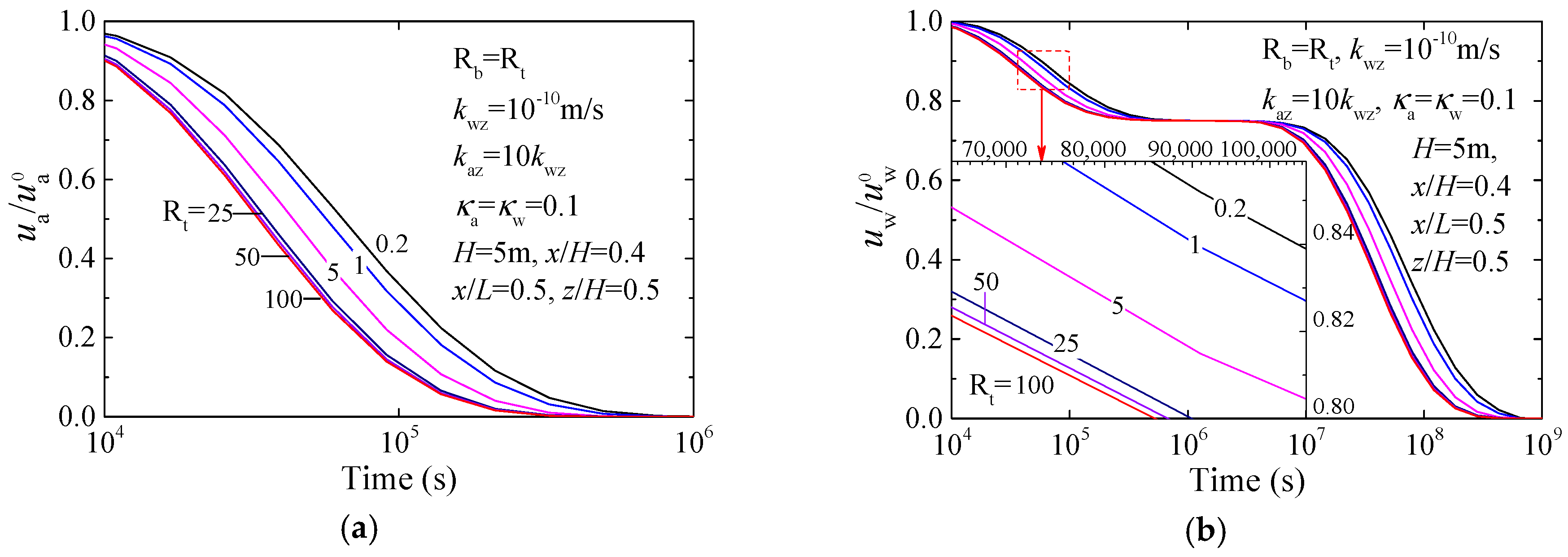
The air-water permeability ratio was defined as the ratio between the vertical permeability coefficient of air phase and that of water phase, i.e., $k_{\mathrm{az}}/k_{\mathrm{wz}}$. Moreover, the anisotropic permeability conditions of these phases were assumed to be the same, i.e., ${\kappa }_{\mathrm{a}}=$${\kappa }_{\mathrm{w}}$. Figure 9 shows the changes of the excess pore-pressures under different values of $k_{\mathrm{az}}/k_{\mathrm{wz}}$, in which the vertical impeded drainage boundaries are given by $R_{\mathrm{b}}=R_{\mathrm{t}}=5$ and $R_{\mathrm{b}}=R_{\mathrm{t}}=\infty$, respectively. The corresponding variations of the soil layer settlement are shown in Figure 10. It can be observed that the air-water permeability ratio had a great influence on the dissipation processes of the excess pore-pressures and the development of the soil layer settlement. Larger $k_{\mathrm{az}}/k_{\mathrm{wz}}$ delivered faster dissipation of the excess pore-air pressure at the later stage, and resulted in faster dissipation of the excess pore-water pressure at the intermediate stage. After that, the excess pore-air pressure was fully dissipated, the plateau period emerged on the normalized curve of the excess pore-water pressure, and then, different curves tended to gradually convergence into a single one (see Figure 9b). A similar characteristic can be found in the normalized curves of the soil layer settlement (see Figure 10). Moreover, the bigger $k_{\mathrm{az}}/k_{\mathrm{wz}}$ can obviously prolong the plateau periods above. In comparison with the results obtained when $R_{\mathrm{b}}=R_{\mathrm{t}}=\infty$, the excess pore-pressures and soil layer settlement obtained when $R_{\mathrm{b}}=R_{\mathrm{t}}$$=5$ were smaller; that is, it needed more time to complete the consolidation process. This phenomenon happened as a result of the impeding effects of the top and bottom drainage boundaries given by $R_{\mathrm{b}}=R_{\mathrm{t}}$$=5$, and it was identical to the results under 1D consolidation with the impeded drainage boundaries [21].

4.3. Consolidation Process with Different Anisotropic Permeability Ratios

In this part, for simplicity, the anisotropic permeability ratio of air phase was only considered to be the same as that of water phase, i.e., ${\kappa }_{\mathrm{a}}=$${\kappa }_{\mathrm{w}}$. The vertical impeded drainage boundaries are given by $R_{\mathrm{b}}=R_{\mathrm{t}}=5$ and $R_{\mathrm{b}}=R_{\mathrm{t}}=\infty$. Figure 11 and Figure 12 illustrate the variations of the excess pore-pressures and the soil layer settlement under different values of ${\kappa }_{\mathrm{a}}=$${\kappa }_{\mathrm{w}}$, respectively. It was obvious that the anisotropic permeability ratio had a great effect on the dissipation processes of the excess pore-pressures and the development of the soil layer settlement. The dissipation with a larger ${\kappa }_{\mathrm{a}}=$${\kappa }_{\mathrm{w}}$ tended to progress relatively faster than that with a smaller one. The reason is that the vertical drains installed in the soil layer provide a shorter drainage path in the horizontal direction, and they allow the excess pore-pressures dissipate faster when ${\kappa }_{\mathrm{a}}=$${\kappa }_{\mathrm{w}}$ is larger. Being the same as the results in Figure 5 and Figure 6, the normalized curves of the excess pore-air pressures were a group of typical inverse S ones with single influence stage while those of the excess pore-water pressures and the soil layer settlements were typical double inverse S curves with two obvious influence stages (see Figure 11 and Figure 12). These curves shifted to the left with an increase of ${\kappa }_{\mathrm{a}}=$${\kappa }_{\mathrm{w}}$. Being the same as those observed in Figure 9 and Figure 10, under a given value of ${\kappa }_{\mathrm{a}}=$${\kappa }_{\mathrm{w}}$, the vertical boundary condition of $R_{\mathrm{b}}$$=R_{\mathrm{t}}=5$ induced slower dissipations of the excess pore-pressures and slower development of the soil layer settlement than the condition of $R_{\mathrm{b}}=R_{\mathrm{t}}=\infty$. For these two boundary conditions, it can be observed that the larger ${\kappa }_{\mathrm{a}}=$${\kappa }_{\mathrm{w}}$ was, the smaller the difference between these results was. That is, the drainage efficiencies of the vertical impeded boundaries affected the 2D consolidation behavior more slightly when ${\kappa }_{\mathrm{a}}=$${\kappa }_{\mathrm{w}}$ was larger (e.g., 4). The reason is that for the scenario of larger ${\kappa }_{\mathrm{a}}=$${\kappa }_{\mathrm{w}}$, most of the excess pore-pressures were dissipated horizontally, and the vertical drainage effect was small and could even be neglected.

4.4. Consolidation Process with Different Spacing-Depth Ratios

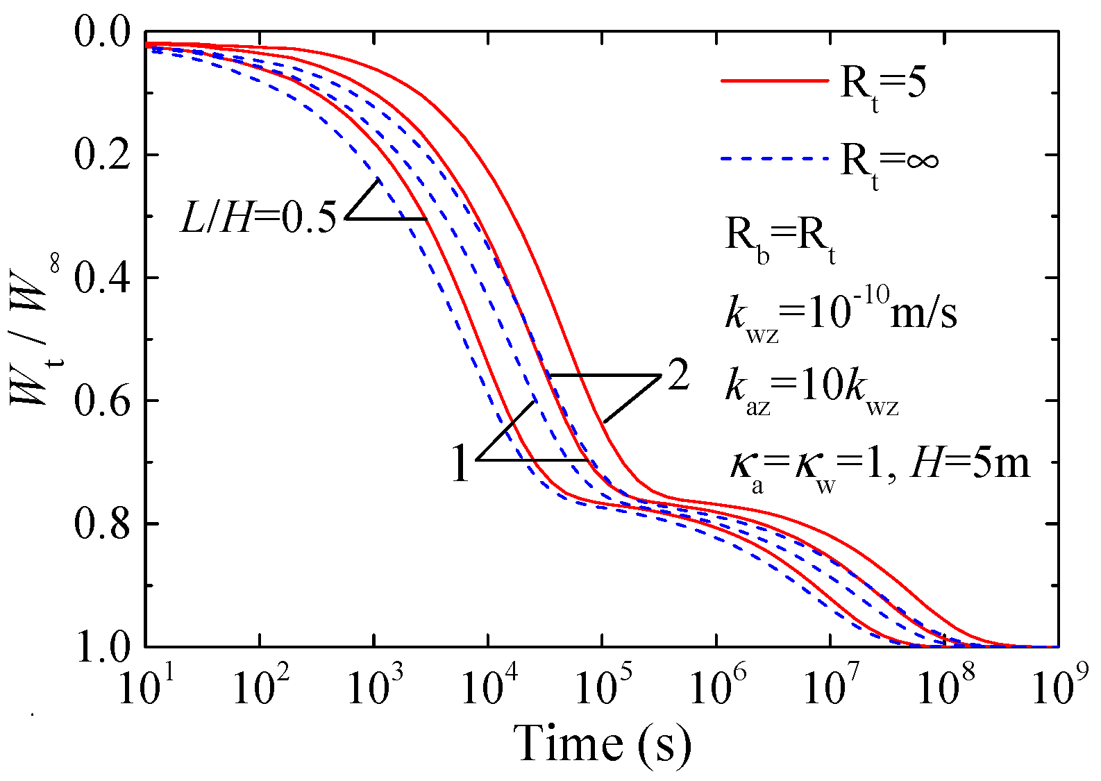
For simplicity, only the isotropic permeability condition for air and water phases was considered in this part, and the vertical impeded drainage boundaries were assumed to be symmetrical. Figure 13 and Figure 14, respectively, illustrate the changes in the excess pore-pressures and soil layer settlement under different spacing-depth ratios (i.e., $L/H$), in which the vertical impeded drainage boundaries are given by $R_{\mathrm{b}}=R_{\mathrm{t}}=5$ and $R_{\mathrm{b}}=R_{\mathrm{t}}=\infty$. It can be observed that a smaller $L/H$ delivered a faster dissipation of the excess-pore pressures due to a shorter horizontal drainage path. As a result, the soil layer settlement develops more quickly. Being the same as the results in Figure 5 and Figure 6, there was a single influence stage on the dissipation pattern of the excess pore-air pressure while there were two obvious influence stages on the dissipation of the excess pore-water pressure and on the development curve of the soil layer settlement (see Figure 13 and Figure 14). Under a given $L/H$, the excess pore-pressures under the vertical boundary condition of $R_{\mathrm{b}}=R_{\mathrm{t}}$$=5$ dissipated more slowly that those under the vertical boundary condition of $R_{\mathrm{b}}=R_{\mathrm{t}}=\infty$. The phenomenon was similar to that observed in Figure 9 and Figure 10. For these two boundary conditions, it was obvious that the difference between their results decreased with the increase of $L/H$. That is, the drainage efficiencies of vertical impeded boundaries had fewer effects on the 2D consolidation behavior when the horizontal drainage path was shorter (e.g., $L/H$ = 0.5). The reason is that most of the excess pore-pressures were dissipated horizontally for the scenario of shorter horizontal drainage path.

5. Conclusions

In this paper, a semi-analytical solution to 2D plane strain consolidation process of unsaturated soil incorporating vertical impeded drainage boundaries was obtained using eigenfunction expansion and Laplace transform techniques. By performing the inversion of Laplace transform, some computations were performed to study the consolidation processes under different drainage efficiencies of the vertical boundaries, air-water permeability ratios, anisotropic permeability ratios and spacing-depth ratios. As a result of the analysis the following conclusions can be drawn.

(a)

The present semi-analytical solution was validated to be consistent with the finite difference solution and the previous analytical solution in the literature, and it is more general in the drainage boundary compared with the existing analytical solution.

(b)

The drainage efficiency of the vertical boundary had a great influence on the dissipation processes of the excess pore-pressures and the development of the soil layer settlement. The larger drainage efficiency delivered the faster dissipation of the excess pore-pressures and the faster development of the soil layer settlement. When the drainage efficiency was large enough (i.e., $R_{\mathrm{t}}\ge 100$ or $R_{\mathrm{b}}\ge 100$), the corresponding boundary can be considered to be fully drained.

(c)

The consolidation process with a larger air-water permeability ratio tended to progress more quickly than that with a smaller one. Either a larger anisotropic permeability ratio (i.e., larger horizontal permeability coefficient) or a smaller spacing-depth ratio delivered faster dissipation of the excess pore pressures and faster development of the soil layer settlement. In comparison with the results under top-base drainage boundary, the impeded drainage boundary with limited drainage efficiency slowed down the consolidation process significantly.

References

- Terzaghi, K. Theoretical Soil Mechanics; Wiley & Sons: New York, NY, USA, 1943. [Google Scholar]
- Schiffman, R.L. Consolidation of soil under time-dependent loading and varying permeability. In Highway Research Board Proceeding, Proceedings of the Thirty-Seventh Annual Meeting of the Highway Research Board, Washington, DC, USA, 6–10 January 1958; Highway Research Board: Washington, DC, USA; Volume 37, pp. 584–617.
- Baligh, M.M.; Levadoux, J.N. Consolidation theory of cyclic loading. J. Geotech. Eng. Div. 1978, 104, 415–431. [Google Scholar]
- Xie, K.H.; Xie, X.Y.; Li, B.H. Analytical theory for one-dimensional consolidation of clayey soils exhibiting rheological characteristics under time-dependent loading. Int. J. Numer. Anal. Met. Geomech. 2008, 32, 1833–1855. [Google Scholar] [CrossRef]
- Liu, J.C.; Griffiths, D.V. A general solution for 1D consolidation induced by depth- and time-dependent changes in stress. Géotechnique 2015, 65, 66–72. [Google Scholar] [CrossRef]
- Scott, R.F. Principles of Soil Mechanics; Addison-Wesley Pub. Co.: Boston, MA, USA, 1963. [Google Scholar]
- Barden, L. Consolidation of compacted and unsaturated clays. Géotechnique 1965, 15, 267–286. [Google Scholar] [CrossRef]
- Barden, L. Consolidation of clays compacted dry and wet of optimum water content. Géotechnique 1974, 24, 605–625. [Google Scholar] [CrossRef]
- Fredlund, D.G.; Hasan, J.U. One-dimensional consolidation theory: Unsaturated soils. Can. Geotech. J. 1979, 16, 521–531. [Google Scholar] [CrossRef]
- Dakshanamurthy, V.; Fredlund, D.G. Moisture and air flow in an unsaturated soil. In Proceedings of the Fourth International Conference on Expansive Soils, Denver, CO, USA, 16–18 June 1980; Volume 1, pp. 514–532. [Google Scholar]
- Ho, L.; Fatahi, B.; Khabbaz, H. Analytical solution for one-dimensional consolidation of unsaturated soils using eigenfunction expansion method. Int. J. Numer. Anal. Met. Geomech. 2014, 38, 1058–1077. [Google Scholar] [CrossRef]
- Zhou, W.H.; Zhao, L.S.; Li, X.B. A simple analytical solution to one-dimensional consolidation for unsaturated soils. Int. J. Numer. Anal. Met. Geomech. 2014, 38, 794–810. [Google Scholar] [CrossRef]
- Shan, Z.D.; Ling, D.S.; Ding, H.J. Exact solutions for one-dimensional consolidation of single-layer unsaturated soil. Int. J. Numer. Anal. Met. Geomech. 2012, 36, 708–722. [Google Scholar] [CrossRef]
- Ho, L.; Fatahi, B.; Khabbaz, H. A closed form analytical solution for two-dimensional plane strain consolidation of unsaturated soil stratum. Int. J. Numer. Anal. Met. Geomech. 2015, 39, 1665–1692. [Google Scholar] [CrossRef]
- Ho, L.; Fatahi, B. Analytical solution for the two-dimensional plane strain consolidation of an unsaturated soil stratum subjected to time-dependent loading. Comput. Geotech. 2015, 67, 1–16. [Google Scholar] [CrossRef]
- Xie, K.H.; Xie, X.Y.; Gao, X. Theory of one dimensional consolidation of two-layered soil with partially drained boundaries. Comput. Geotech. 1999, 24, 265–278. [Google Scholar] [CrossRef]
- Gray, H. Simultaneous consolidation of contiguous layers of unlike compressible soils. Trans. ASCE 1945, 110, 1327–1356. [Google Scholar]
- Mesri, G. One-dimensional consolidation of a clay layer with impeded drainage boundaries. Water Resour. Res. 1973, 9, 1090–1093. [Google Scholar] [CrossRef]
- Schiffman, R.L.; Stein, J.R. One-dimensional consolidation of layered system. J. Soil. Mech. Found. Div. ASCE 1970, 96, 1090–1093. [Google Scholar]
- Cai, Y.Q.; Liang, X.; Wu, S.M. One-dimensional consolidation of layered soils with impeded boundaries under time-dependent loadings. Appl. Math. Mech. Engl. 2004, 25, 937–944. [Google Scholar]
- Wang, L.; Sun, D.A.; Xu, Y.F. Semi-analytical solutions to one-dimensional consolidation for unsaturated soils with semi-permeable drainage boundary. Appl. Math Mech. Engl. 2017, 38, 1439–1458. [Google Scholar] [CrossRef]
- Wang, L.; Sun, D.A.; Li, L.Z.; Li, P.C.; Xu, Y.F. Semi-analytical solutions to one-dimensional consolidation for unsaturated soils with symmetric semi-permeable drainage boundary. Comput. Geotech. 2017, 89, 71–80. [Google Scholar] [CrossRef]
- Wang, L.; Sun, D.A.; Qin, A.F. Semi-analytical solution to one-dimensional consolidation for unsaturated soils with semi-permeable drainage boundary under time-dependent loading. Int. J. Numer. Anal. Met. Geomech. 2017, 41, 1636–1655. [Google Scholar] [CrossRef]
- Crump, K.S. Numerical inversion of Laplace transform using a Fourier series approximation. JACM 1976, 23, 89–96. [Google Scholar] [CrossRef]
- Goode, S.W. Differential Equations and Linear Algebra, 2nd ed.; Prentice-Hall Inc.: Upper New Jersey River, NJ, USA, 2000. [Google Scholar]
- Zwillinger, D. Handbook of Differential Equations, 3rd ed.; Academic Press: San Diego, CA, USA, 1997. [Google Scholar]
- Durbin, F. Numerical inversion of Laplace transforms: An efficient improvement to Dubner and Abate’s method. Comput. J. 1974, 17, 371–376. [Google Scholar] [CrossRef]
- Wang, L.; Sun, D.A.; Li, P.C.; Xie, Y. Semi-analytical solution for one-dimensional consolidation of fractional derivative viscoelastic saturated soils. Comput. Geotech. 2017, 83, 30–39. [Google Scholar] [CrossRef]
- Morton, K.W.; Mayers, D. Numerical Solution of Partial Differential Equations: An Introduction, 2nd ed.; Cambridge University Press: Cambridge, UK, 2005. [Google Scholar]
- Croft, D.R.; Lilley, D.G. Heat Transfer Calculations Using Finite Difference Equations; Applied Science Publishers LTD: London, UK, 1977. [Google Scholar]
Figure 1.
Two-dimensional (2D) consolidation system of unsaturated soil with vertical impeded drainage boundaries.
Figure 2.
Excess pore-pressures under top-base drainage boundary calculated from semi-analytical solution (SAS) and previous analytical solution (PAS): (a) air phase and (b) water phase.
Figure 3.
Excess pore-pressures under top drainage boundary calculated from semi-analytical solution (SAS) and previous analytical solution (PAS): (a) air phase and (b) water phase.
Figure 4.
Excess pore-pressures under impeded drainage boundary calculated from semi-analytical solution (SAS) and finite difference solution (FDS): (a) air phase and (b) water phase.
Figure 5.
Variations of excess pore-pressures under symmetrical vertical impeded drainage boundary with different drainage efficiencies: (a) air phase and (b) water phase.
Figure 6.
Variations of soil layer settlement under symmetrical vertical impeded drainage boundary with different drainage efficiencies.
Figure 7.
Variations of excess pore-pressures under asymmetrical vertical impeded drainage boundary with different drainage efficiencies: (a,b) and (c,d) .
Figure 8.
Variations of soil layer settlement under asymmetrical vertical impeded drainage boundary with different drainage efficiencies: (a) and (b) .
Figure 9.
Variations of excess pore-pressures under vertical impeded drainage boundary with different air-water permeability ratios: (a) air phase and (b) water phase.
Figure 10.
Variations of soil layer settlement under vertical impeded drainage boundary with different air-water permeability ratios.
Figure 11.
Variations of excess pore-pressures under vertical impeded drainage boundary with different anisotropic permeability ratios: (a) air phase and (b) water phase.
Figure 12.
Variations of soil layer settlement under vertical impeded drainage boundary with different anisotropic permeability ratios.
Figure 13.
Variations of excess pore-pressures under vertical impeded drainage boundary with different spacing-depth ratios: (a) air phase and (b) water phase.
Figure 14.
Variations of soil layer settlement under vertical impeded drainage boundary with different spacing-depth ratios.
© 2018 by the authors. Licensee MDPI, Basel, Switzerland. This article is an open access article distributed under the terms and conditions of the Creative Commons Attribution (CC BY) license (http://creativecommons.org/licenses/by/4.0/).
Share and Cite
MDPI and ACS Style
Huang, M.; Li, D. 2D Plane Strain Consolidation Process of Unsaturated Soil with Vertical Impeded Drainage Boundaries. Processes 2019, 7, 5. https://doi.org/10.3390/pr7010005
AMA Style
Huang M, Li D. 2D Plane Strain Consolidation Process of Unsaturated Soil with Vertical Impeded Drainage Boundaries. Processes. 2019; 7(1):5. https://doi.org/10.3390/pr7010005
Chicago/Turabian StyleHuang, Minghua, and Dun Li. 2019. "2D Plane Strain Consolidation Process of Unsaturated Soil with Vertical Impeded Drainage Boundaries" Processes 7, no. 1: 5. https://doi.org/10.3390/pr7010005
Note that from the first issue of 2016, this journal uses article numbers instead of page numbers. See further details here.