Fault Identification Using Fast k-Nearest Neighbor Reconstruction


School of Engineering, Huzhou University, Huzhou 313000, China
*
Authors to whom correspondence should be addressed.
Processes 2019, 7(6), 340; https://doi.org/10.3390/pr7060340
Submission received: 4 May 2019
/
Revised: 27 May 2019
/
Accepted: 31 May 2019
/
Published: 5 June 2019
(This article belongs to the Collection Process Data Analytics)
Abstract
:Data with characteristics like nonlinear and non-Gaussian are common in industrial processes. As a non-parametric method, k-nearest neighbor (kNN) rule has shown its superiority in handling the data set with these complex characteristics. Once a fault is detected, to further identify the faulty variables is useful for finding the root cause and important for the process recovery. Without prior fault information, due to the increasing number of process variables, the existing kNN reconstruction-based identification methods need to exhaust all the combinations of variables, which is extremely time-consuming. Our previous work finds that the variable contribution by kNN (VCkNN), which defined in original variable space, can significantly reduce the ratio of false diagnosis. This reliable ranking of the variable contribution can be used to guide the variable selection in the identification procedure. In this paper, we propose a fast kNN reconstruction method by virtue of the ranking of VCkNN for multiple faulty variables identification. The proposed method significantly reduces the computation complexity of identification procedure while improves the missing reconstruction ratio. Experiments on a numerical case and Tennessee Eastman problem are used to demonstrate the performance of the proposed method.
1. Introduction
Process monitoring combined with advanced process control technologies guarantee the long-term safe operation and efficient production of the modern industrial processes. The multivariate statistical process monitoring (MSPM) methods are important for the process industry [1,2,3]. As the increasingly changing in its complexity of modern industrial processes, the measurement data obtained from these processes have complex characteristics, such as nonlinear, multi-mode, and non-Gaussian [2,4,5,6,7]. Several variants of MSPM methods have also been developed to handle the data set with these characteristics [8,9,10,11,12,13,14]. However, these MSPM methods cannot provide satisfied monitoring results when the measurement data have all these complicated characteristics. To explicitly account for these characteristics, He and Wang [7] developed an alternative fault detection method based on k-nearest neighbor rule (FD-kNN), it uses the kNN distance as an index to measure the discrepancy between the online data sample and the normal operation conditions (NOC) data samples. Compared to those of MSPM methods, FD-kNN has shown its superiority in analyzing nonlinear, multi-mode, and non-Gaussian distribution data [7,15,16,17,18,19]. Moreover, as a nonlinear classifier, kNN is naturally possible to handle nonlinearity in the data [7]. In addition, FD-kNN has no constrains on the distribution of data, thus this makes it could be used in many applications.
Once a fault is detected in the process, to identify the faulty variables is useful for finding the root cause and also important for the process recovery. In the frame of MSPM, many contribution analysis methods, such as contribution plot [20], reconstruction-based contribution [21,22,23], and several variants [24], have been proposed to solve the problem of faulty variable identification. However, these method suffer from smearing effect due to the inherent linear transformation in the definition of contribution index [19,25], thus increasing the false identification ratio [26,27]. In addition, the control limit for each variable contribution is inaccurate because linear Gaussian assumption on NOC data usually contradicts with practical industrial processes. This makes these contribution analysis methods more difficult to identify multiple faulty variables. In previous work [19], we defined a new variable contribution by kNN in the original variable space, which does not suffer from the smearing effect. Under the assumption that the magnitude of the fault is significantly larger than the absolute distance between the online sample and its kNN in terms of each variable, VCkNN can guarantee that the contribution values of faulty variables are always larger than that of the rest non-faulty variables.
Wang et al. [28] developed an algorithm for fault variables identification based on kNN reconstruction (FVI-kNN). In FVI-kNN, each variable is sequentially estimated by the rest variables using kNN regression; then m (i.e., the number of the variables) reconstructed samples can be obtained by replacing the original variables with their estimation, respectively. Then, FD-kNN is used to re-detect these m reconstruction samples. The one with maximum reduction in the detection index (MRI) and is simultaneously smaller than the detection threshold is considered the faulty variable; otherwise, at least two of them are faulty variables. To further identify the root cause, the reconstruction procedure need to continue by replacing each of the two variables using previous estimations, then re-detecting these reconstruction samples again by FD-kNN and identifying the faulty variables based on MRI. The reconstruction procedure will continue until the true faulty variables are determined.
In FVI-kNN, however, the approach of reconstructing fault sample when there are more than one faulty variable is unreasonable and inaccurate. This is because the rest variables contain faulty variable when estimating each variable by kNN regression. In other words, abnormal predictors cannot give accurate response. Therefore, inaccurate sample reconstruction cannot provide reliable identification results of faulty variables. To address this drawback, we have presented an improved FVI-kNN (IFVI-kNN) method [29], where the possible variables are re-estimated simultaneously in the case of multiple faulty variables. This guarantee no mutual influence in the estimations of the possible faulty variables. Thus, the IFVI-kNN fixes this drawback and improve its reliability for faulty variables identification.
Without prior fault information, however, the identification procedure of either FVI-kNN [28] or IFVI-kNN [29] is extremely time-consuming. For an industrial process with m monitoring variables, when any fault affects q of the m variables, the times of sample reconstruction required by these two methods [28,29] is . For example, a chemical process contains 50 variables and four of them were affected by a fault, thus the times of sample reconstruction required are 230,300. In this situation, it is difficult to rapidly identify the faulty variables and the root cause of the fault.
We have proven that the VCkNN is able to provide a reliable ranking of the variable contribution to the fault. This ranking can be used as a credible guide for the variables selection in the reconstruction procedure. Therefore, the efficiency of the identification procedure is expected to be improved by adopting a reliable strategy for variables selection. The main aim of this paper is to provide a fast kNN reconstruction method by virtue of VCkNN for multiple faulty variables identification. The proposed method sequentially eliminates the effect of the faulty variable according to the ranking of VCkNN and reconstructs the fault sample by replacing the faulty variables with their kNN estimation. The faulty variables are determined if the reconstruction sample is brought back to the normal region. The proposed method significantly improves the efficiency of identification procedure while reduces the missing reconstruction ratio (MRR). Numerical case study and Tennessee Eastman (TE) problem are used to demonstrate the superiority of the proposed method.
2. Methods
This section contains three parts. In the first part, a brief review of FD-kNN is given. The VCkNN used to guide the variable selection in the reconstruction procedure is introduced in second subsection. In the last part, we present our proposed method.
2.1. Fault Detection Method Based on kNN Rule
The FD-kNN is developed to handle the data with complex characteristics, such as nonlinear, non-Gaussian, and multimode. The idea behind FD-kNN is that the normal sample is similar to the NOC sample, while the fault sample is far from the NOC samples. Hence, the pairwise distances between samples in a small region can be a decent index for fault detection. Here, we review the procedure of this algorithm, the details can be referred to [7,15].
- Off-Line Model building
- Find k nearest neighbors for each sample, , in the normalized NOC data set by using Euclidean distance.where is the distance between and its jth nearest neighbor.
- Calculate the average kNN distance (it may not be a rigorous mathematical distance) of the sampleHere, is the average squared distance between sample and its k nearest neighbors. The average kNN distance is used as the detection index.
- Determine the detection thresholdThe threshold with significance level can be determined by the -empirical quartile of [16]where is the ranking of in ascending order. takes the integer part from .
- Online monitoringWhen a normalized online sample is obtained, e.g., ,
2.2. Variable Contribution by kNN
Although the kNN rule has been successfully applied to detect the abnormal in the process industry [7,15,16,17,18], how to identify the faulty variables using by kNN method without prior fault information is still a challenge problem.
In our previous work [19], we have proposed a new variable contribution based on the kNN distance. This contribution index improves the successful identification ratio of faulty variable. Similar to the contribution analysis method, the VCkNN is designed by decomposing the kNN distance of into a sum of m variable contribution [19]
where is the ith column of the identity matrix. The contribution of ith variable to the detection index is
It can be seen that the sum of the VCkNNs is equal to the detection index, i.e., . Note that VCkNN is defined in original variable space and each variable contribution is not related to the other variables. In contrast, the variable contributions given by traditional contribution analysis methods are correlated which tend to misidentify faulty variables.
The VCkNN has been proven to give reliable ranking of variable contributions. Specifically, the contributions of true faulty variables given by VCkNN are always larger than the rest of non-faulty variables [19]
where F and are the set of faulty variables and non-faulty variables, respectively.
This advantage of VCkNN can be very useful in improving the efficiency of the identification procedure of faulty variables. In the next subsection, we will incorporate VCkNN into the reconstruction procedure of fault samples so that the faulty variables can be identified efficiently.
3. The Proposed Method for Fault Variable Identification by kNN Reconstruction
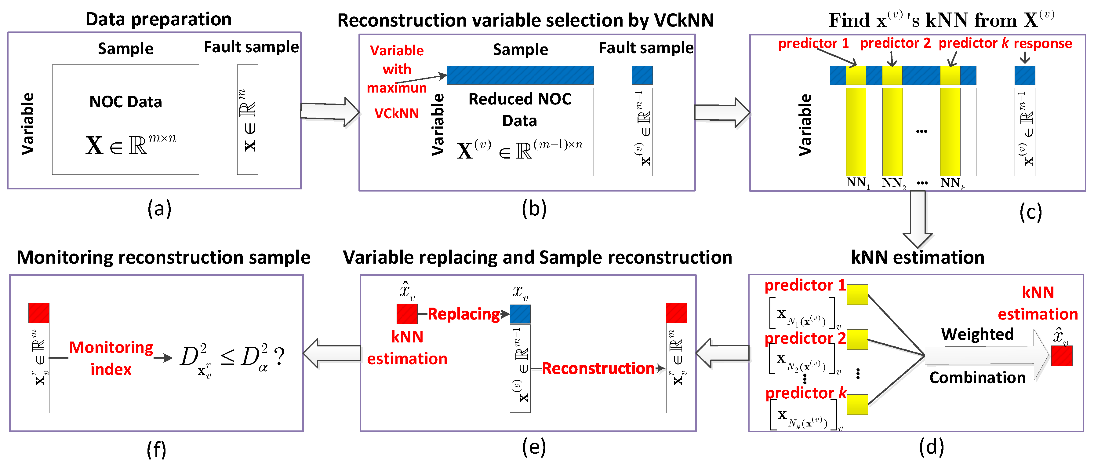
Many studies indicate that efficient variable selection used in the reconstruction of fault samples can improve the efficiency of identification procedure of faulty variables [30,31]. Inspired by this idea, this paper develops a fast identification algorithm for faulty variables based on kNN estimation using the ranking of VCkNN. The flowchart of the main identification procedure is shown in Figure 1.
The first step in Figure 1a is data preparation. The sample , which is far from the NOC data measured by FD-kNN, is fault sample.
The second step in Figure 1b is to determine the variable (the one with maximum VCkNN) used in the following reconstruction procedure, then splitting the NOC data and fault sample into two parts, i.e., with faulty variable (blue) and without faulty variable (white), respectively.
The third step in Figure 1c is to find the kNN of reduced fault sample from reduced NOC data . The neighbors’ have their corresponding value in the selected variable (i.e., the three yellow small squares), and will be used as the predictors in the kNN estimation.
The fourth step in Figure 1d is to predict the selected possible faulty variable using those predictors by a weighted combination.
After obtaining the kNN estimation of this selected variable, the next step in Figure 1e is to reconstruct the fault sample by replacing the selected variable by its kNN estimation. The monitoring index of this reconstructed sample will be calculated and compared with the detection threshold used in FD-kNN. If it is smaller than the threshold, then the selected variable is identified as the fault variable; otherwise the identification procedure will continue from the step two in Figure 1b.
In this situation, the difference with the first round of reconstruction is that two reconstruction variables (with the first two largest VCkNN) will be selected and simultaneously estimated by kNN. After obtaining the kNN estimation of these two possible faulty variables, the fault sample will be again reconstructed by replacing these two variables with their kNN estimations. Then, the monitoring index of the new reconstruction sample will be computed again and compared with the threshold. If it is smaller than the threshold, then these two variables are identified as faulty variables; otherwise the identification procedure needs to continue until the true faulty variables are determined.
To describe the identification procedure of the proposed algorithm in a formal mathematical language:
Set loop variable . For a fault sample , i.e.,
- Calculate the ranking of VCkNN forwhere is the variable with i-th largest contribution.
- Divide the data into two partsAdd into candidate variable set and divide the NOC data and fault sample according to the candidate setwhere is the cardinality of set v.
- Find ’s kNN, , from the reduced NOC data
- Predict the variables in set vwhere is the normalized weight obtained from the negative exponential distance between and its l-th nearest neighbor from . is the label of ’s lth nearest neighbor in reduced training set . represents the -th entry of the sample .
- Obtain reconstruction sampleReconstructing the fault sample by replacing its entries with their estimations .
- Faulty variables identificationCalculating detection index of the reconstructed sample using Equation (2), . If , then the faulty variables are determined as those variables in set v; otherwise, return to step 2 and .
The main difference between the proposed method and FVI-kNN lies in the following aspects:
1. The way of variable selection used in the proposed method is depends on the VCkNN. Under the guide of an accurate VCkNN, the proposed method only needs the same number of loop of fault sample reconstruction as the number of faulty variables. In contrast, FVI-kNN and IFVI-kNN need to exhaust the combinations of variables.
2. The kNN estimation for multiple variables used in the proposed methods is more reasonable than FVI-kNN. The predictors used in the estimation do not contain the faulty variables, which provides more accurate estimations for multiple variables and enhances the reliability of the proposed method for the identification of faulty variables.
4. Results
In this section, the proposed method is demonstrated by a numerical case study and TE problem.
4.1. Numerical Simulation
To compare the proposed method with the FVI-kNN based on the identical simulation model under the same conditions, the following data generation model as that in Ref. [28] is used in this case study
where are Gaussian noises. The seven variables are generated from two latent variables and . Obviously, the distribution of the data generated based on this model are non-Gaussian and the relation between the seven variables are nonlinear. Hence, the case study is applicable for verifying the performance of those methods including the proposed approach on fault detection and identification.
Five hundred NOC samples are generated from system Equation (8). Another 500 NOC samples are generated as test data for simulating the fault data. Three cases, where case 1 and case 2 are a step-type fault and case 3 is a ramp-type fault, are used to illustrate the performance of the proposed method. The number of the neighbors k is 15 and the significance level .
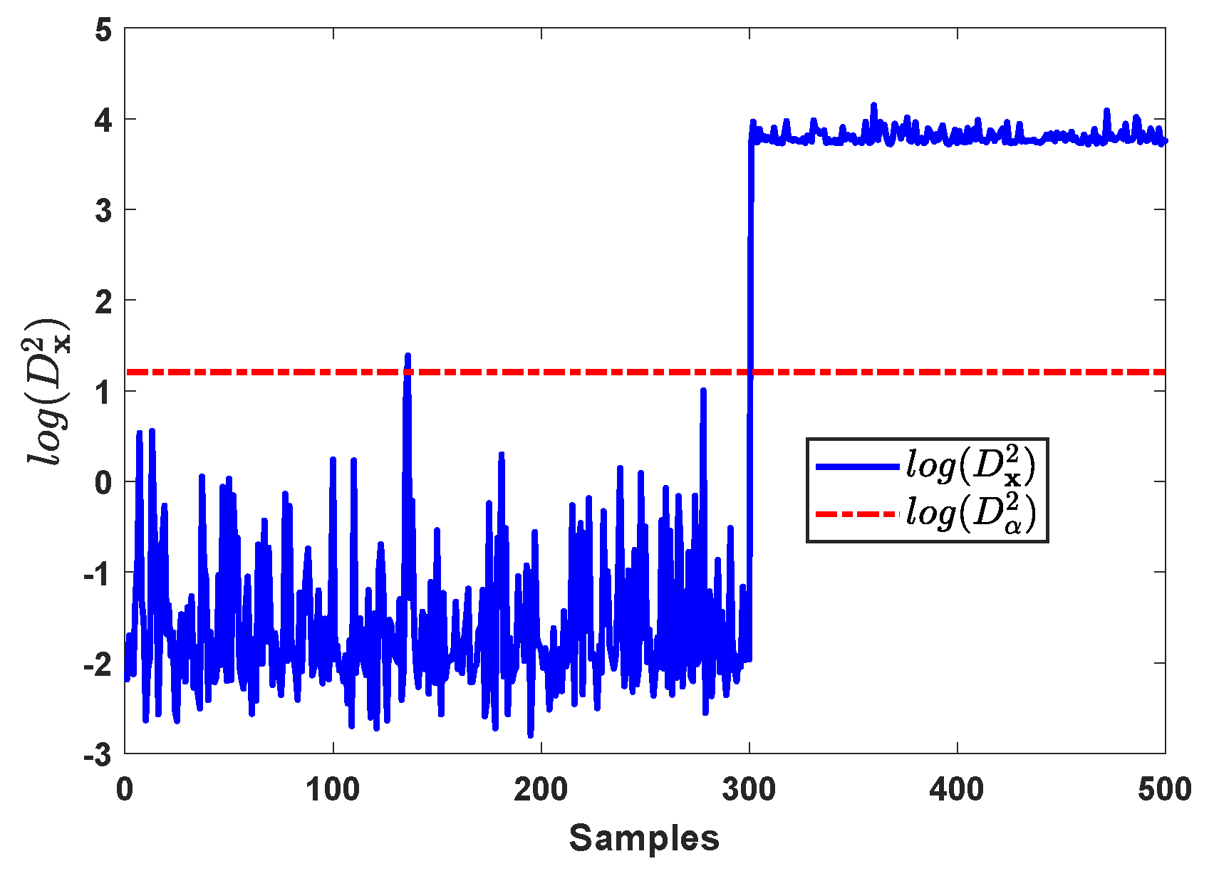
Case 1
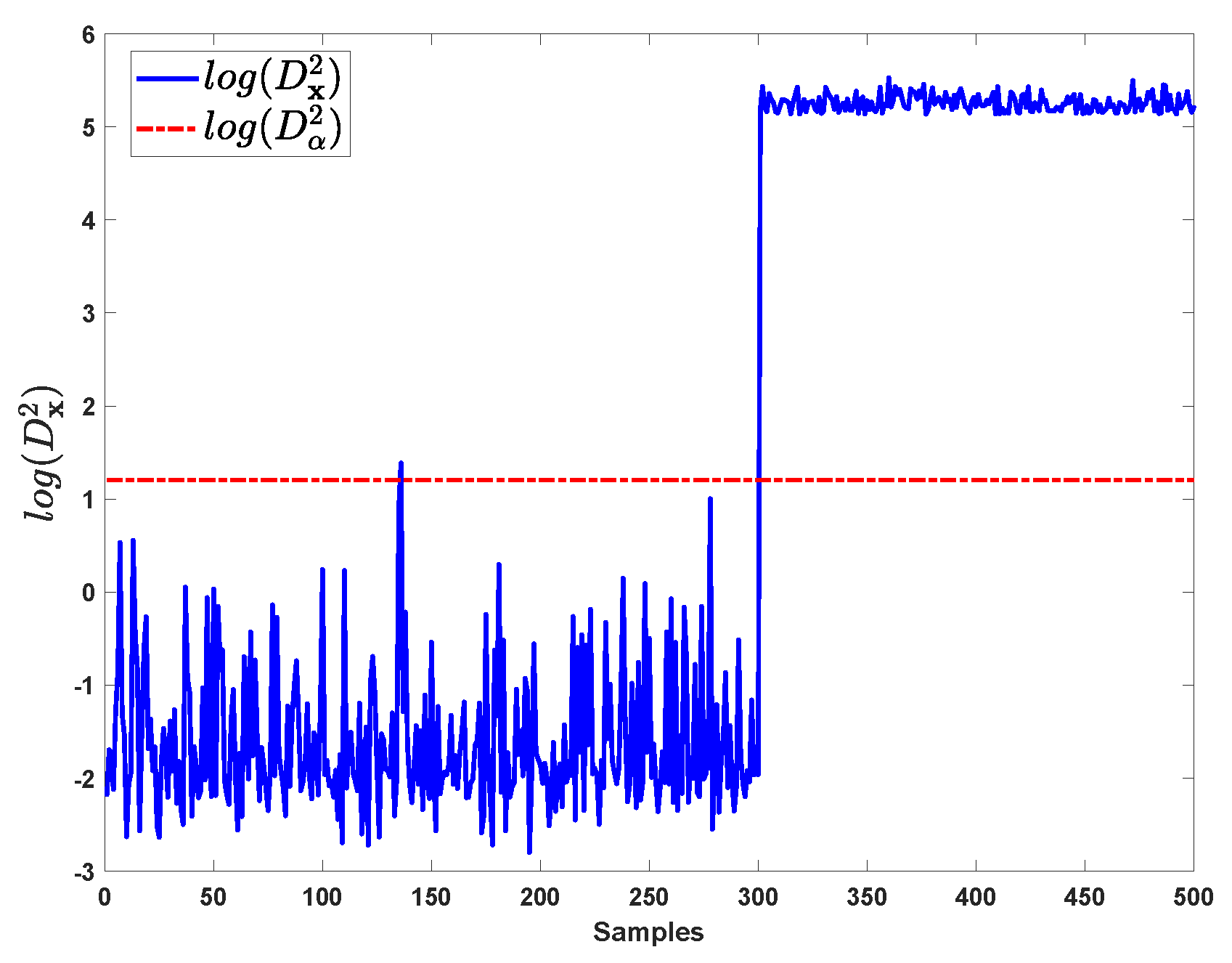
In case 1, step changes are added on and starting from the 301st sample with the magnitudes are all equal to 2. The fault detection results by kNN for case 1 are shown in Figure 2, this step fault is immediately detected at the 301st sample.
Without the prior fault information, the identification procedure is completed by firstly finding the main responsible variables from VCkNN, then sequentially eliminating effect of these candidate variables on fault samples and reconstructing the normal samples, and finally determining the faulty variables by monitoring whether the reconstructed samples are below the detection threshold.
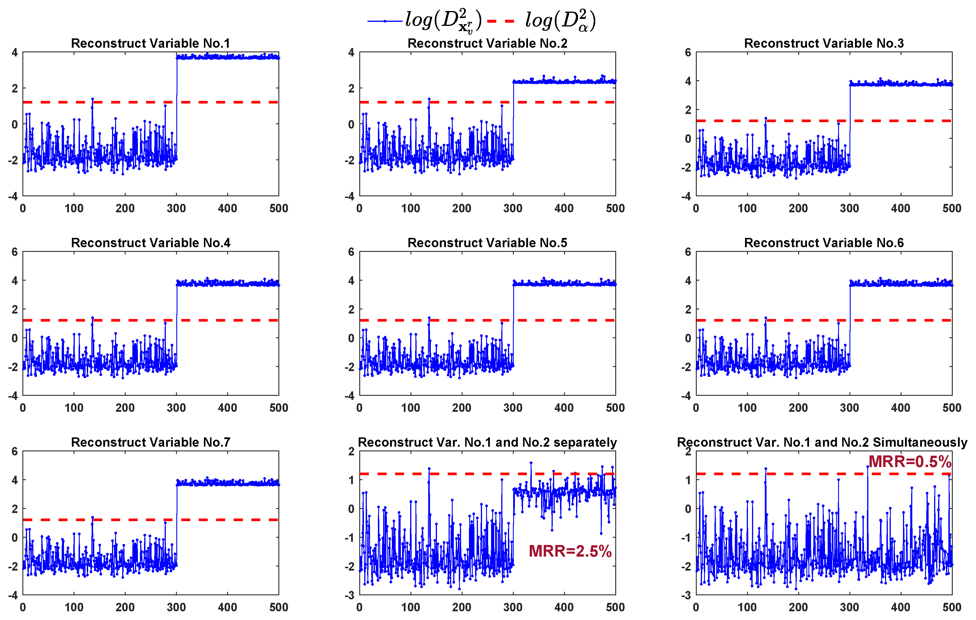
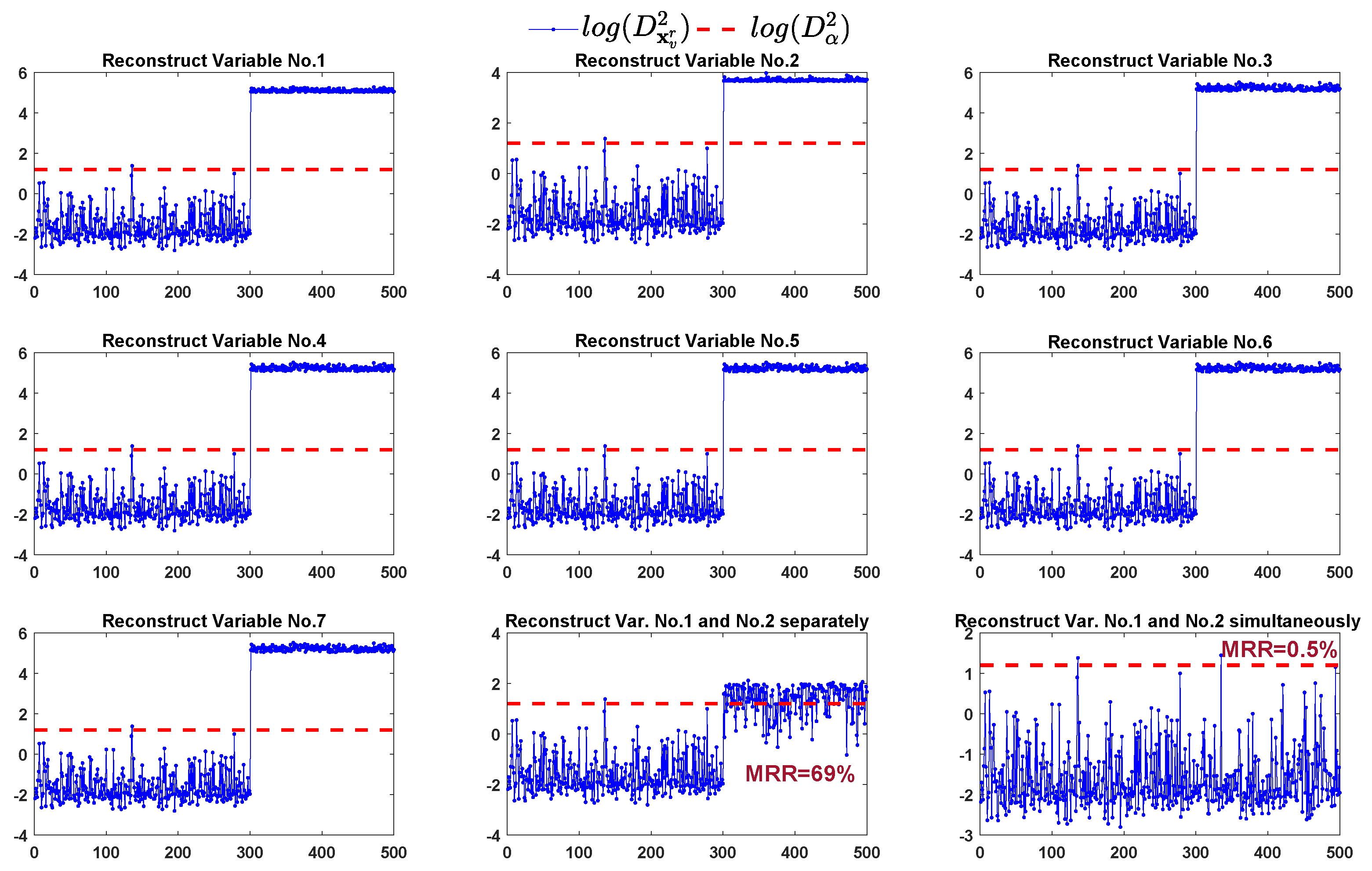
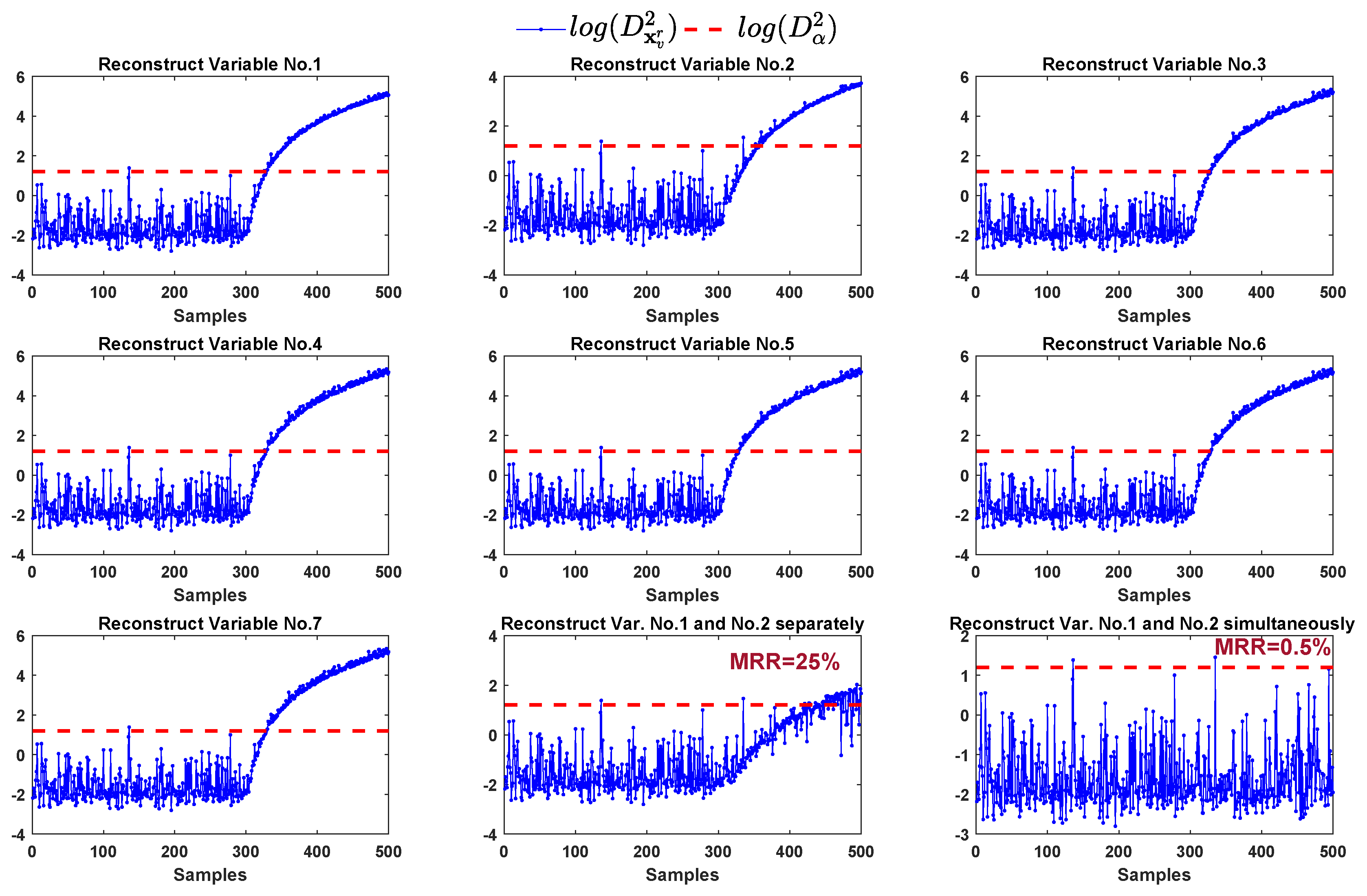
We apply those identification methods to find the faulty variables. The FVI-kNN firstly reconstructs the fault samples by estimating and replacing each variable. Then, the average kNN distance of the reconstructed samples is computed and compared with the detection threshold. The monitoring results of reconstruction samples are shown in Figure 3. From the first seven sub-graphs of Figure 3, we can see that only replacing one variable cannot bring the reconstructed samples back to the normal region. In this situation, the FVI-kNN has to continue the reconstruction procedure by exhausting all the combination of any two variables using their previous single-variable estimations. The FVI-kNN can provide satisfied MRR only when the combination of variable no.1 and variable no.2 are selected for reconstruction. In the 8th sub-graph (row 3, column 2) of Figure 3, the monitoring results of the reconstructed samples by replacing variable no.1 and variable no.2 separately show that most of the fault samples are brought back to the normal region.
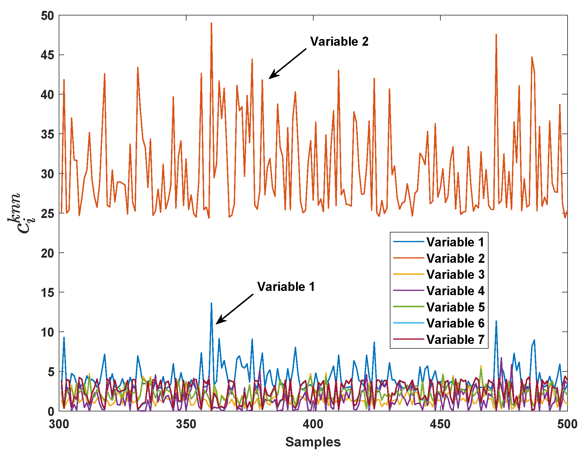
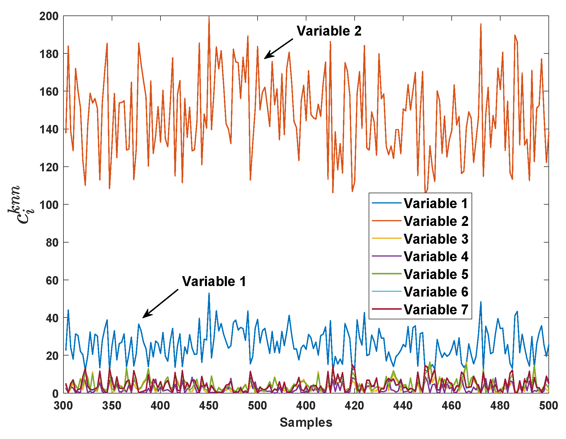
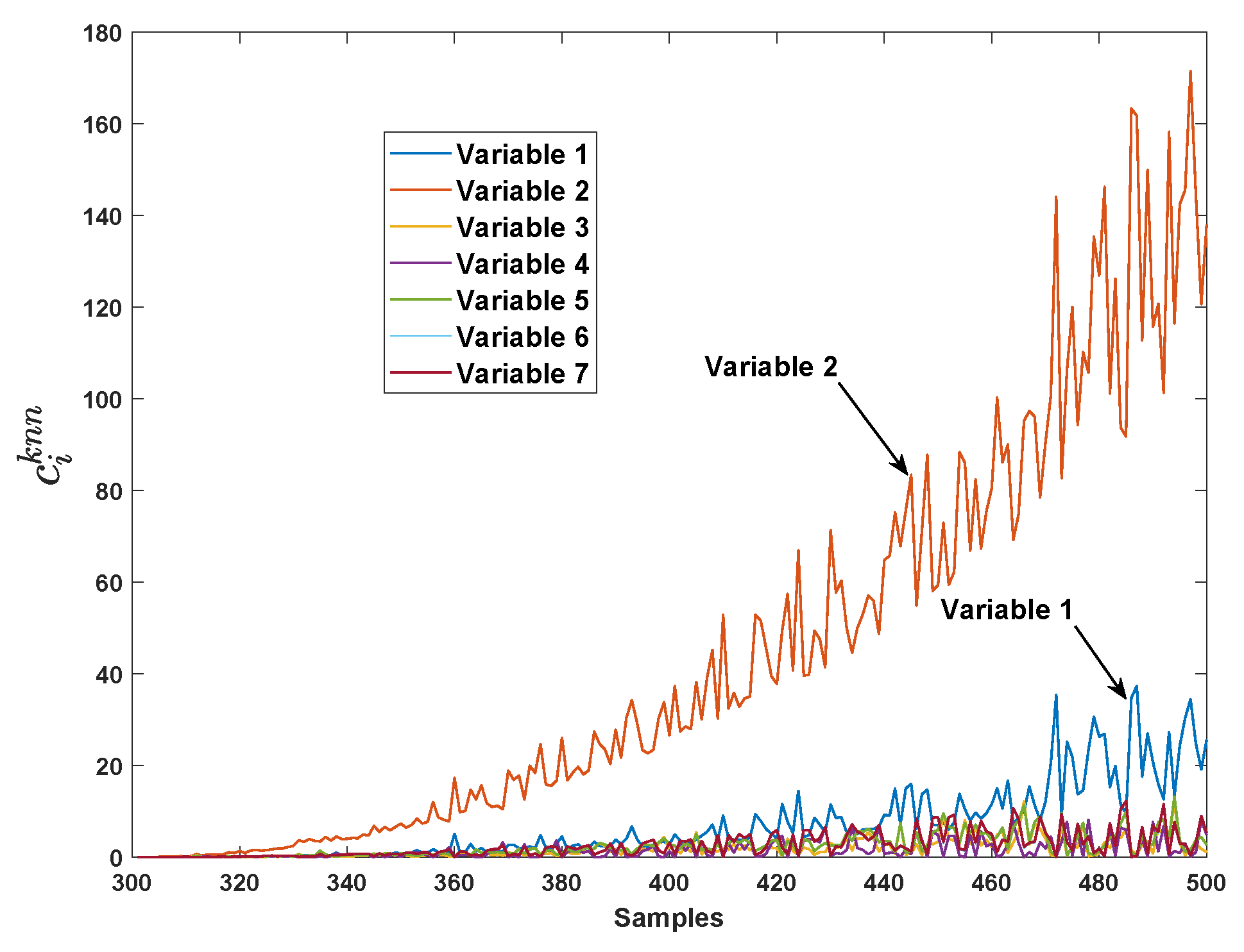
The proposed method firstly compute the VCkNN of each variable from 301st sample. The result is depicted in Figure 4. It can be seen that the VCkNN of variable no.2 () is significantly larger than other VCkNNs, and the VCkNN of variable no.1 () is slightly larger than the rest.
With the help of the VCkNNs, the proposed method firstly reconstructs the fault samples by estimating and replacing the variable with largest VCkNN (i.e., variable no.2 in this case). Then, the average kNN distance of the reconstructed samples is computed and compared with the detection threshold. The monitoring result of reconstruction samples is the same as that in the 2nd sub-graph (row 1, column 2) of Figure 3. From this sub-graph, we can see that only replacing variable no.2 in the reconstruction cannot bring the fault samples back to the normal region. According to the proposed identification approach, in the second loop of reconstruction, the fault samples are then reconstructed by simultaneously estimating and replacing variable no.2 and variable no.1 (i.e., variables with the first two largest VCkNNs). Then, the monitoring result is shown in the last sub-graph (row 3, column 3) of Figure 3, it can be seen that the reconstructed samples by estimating and replacing variable no.2 and variable no.1 simultaneously are all brought back to the normal region except only one fault sample.
In summary, either separately or simultaneously estimating the faulty variables can correctly identify the faulty variables in case 1. However, our proposed method still gives lower MRR (0.5% vs. 2.5%). In addition, the proposed method only needs reconstruction twice to identify the faulty variables while the FVI-kNN needs at least eight times reconstruction (twenty-eight times in the worst case) before the fault variables can be identified. The computation time used by the proposed method is significantly reduced compared to that of the FVI-kNN.
Case 2
The difference between case 2 and case 1 is that the magnitudes of the step changes are all equal to 4. The fault detection results by kNN for case 2 are shown in Figure 5, this step fault is also immediately detected at the 301st sample.
In Figure 6, the VCkNN of each variable from 301st sample are depicted. It can be seen that the VCkNN of variable no.2 () and variable no.1 () is significantly larger than other VCkNNs.
According to the VCkNNs, the proposed method should first try to reconstruct fault samples by estimating and replacing variable no.2 and re-detect the reconstructed samples by kNN. If this cannot bring most of the fault samples back to the normal region, then continue this procedure and reconstruct the fault samples by estimating and replacing variable no.2 and variable no.1 simultaneously until the faulty variables are identified.
The monitoring results of reconstruction samples are shown in Figure 7. From the first seven sub-graphs of Figure 7, we can see that only replacing one variable cannot bring the reconstructed samples back to the normal region. In the 8th sub-graph (row 3, column 2) of Figure 7, the monitoring results of the reconstructed samples by estimating and replacing variable no.1 and variable no.2 separately show that more than half of the fault samples (MRR = 69%) cannot be brought back to the normal region. This illustrates that the way of estimation for the case of multiple faulty variables is unreasonable and inaccurate. On the contrary, our proposed method provides the results in the last sub-graph (row 3, column 3) of Figure 7, the monitoring results show that the way of estimating and replacing variable no.1 and variable no.2 simultaneously can bring almost all the fault samples back to the normal region (MRR = 0.5%).
Consider the computation time of the identification algorithms, the FVI-kNN needs at least eight times reconstructions (twenty-eight times in the worst case) before the faulty variables can be identified. The proposed method only needs reconstruction twice to identify the faulty variables. Therefore, the computation time used by the proposed method is significantly reduced compared to that of the FVI-kNN.
Case 3
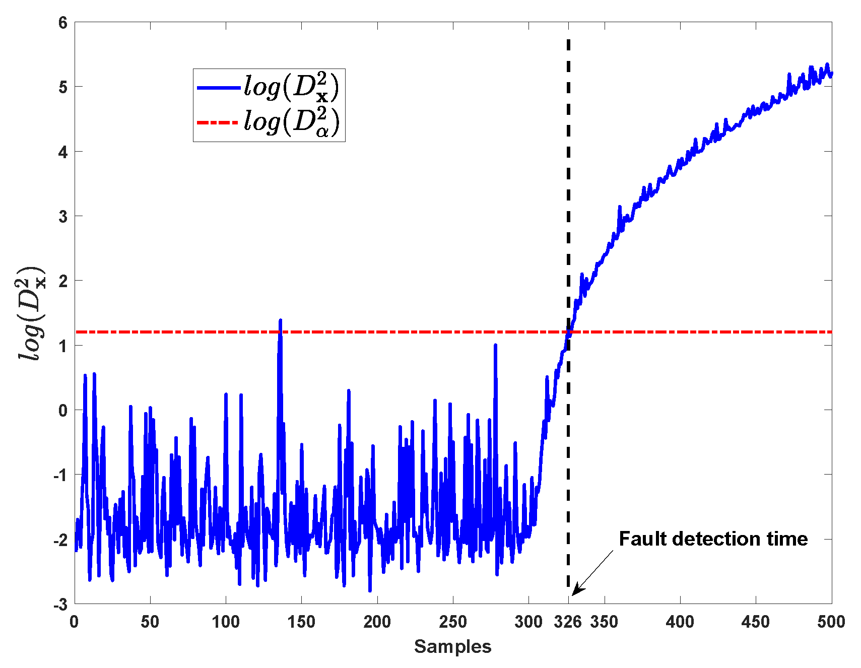
In case 3, ramp-type fault are added on and from the 301st sample with the magnitudes changing in the form of , where i is the sampling time. The fault detection results by kNN for this case are shown in Figure 8, this ramp fault is detected by kNN at the 326th sample.
In Figure 9, the VCkNN of each variable from 301st sample are depicted. It reveals that the VCkNN of variable no.2 () and variable no.1 () is gradually larger than other VCkNNs since the ramp fault occurs at the 301st sample.
The reconstruction results in Figure 10 show that the proposed method successfully identify the faulty variables, i.e., variable no.1 and no.2, while the FVI-kNN still has an unacceptable high MRR(25%). Hence, the FVI-kNN cannot provide correct identification result.
Table 1 summarizes the results of these three numerical cases, it shows that the strategy of reconstructing fault samples used in our proposed method is correct and effective. In addition, the method in Ref. [28] have to inspect at least eight monitoring charts before the fault variables can be identified. In contrast, our proposed method only needs two monitoring charts to find the faulty variables. The faults in these three cases only affect two of the seven process variables. This demonstrates the efficiency of our proposed method. For the practical large-scale industrial processes, the number of process variables and the faulty variables are huge. In this situation, the advantages of our proposed method are obvious.
4.2. TE Process
To further compare our proposed method with existing method, the experiments on TE benchmark chemical process are also conducted. The TE problem a benchmark dataset [32]. This process is composing of five units: reactor, condenser, compressor, separator, and stripper. The TE problem contains 53 variables with 21 faults involving complex process dynamics and variable non-linearity, which is suitable for verifying the fault identification efficiency of the proposed method. The details of TE process can be found in Ref. [32,33]. The faults involved are step disturbance, random variation, slow drift, and sticking, etc. In our experiments, thirty-three variables are used including the first 22 measurement variables and 11 manipulated variables. The fault #4 (Step), fault #11 (Random Variation), and fault #14 (Sticking) are used to demonstrate the effectiveness of the proposed method. The data set can be obtained online [34].
Fault 4
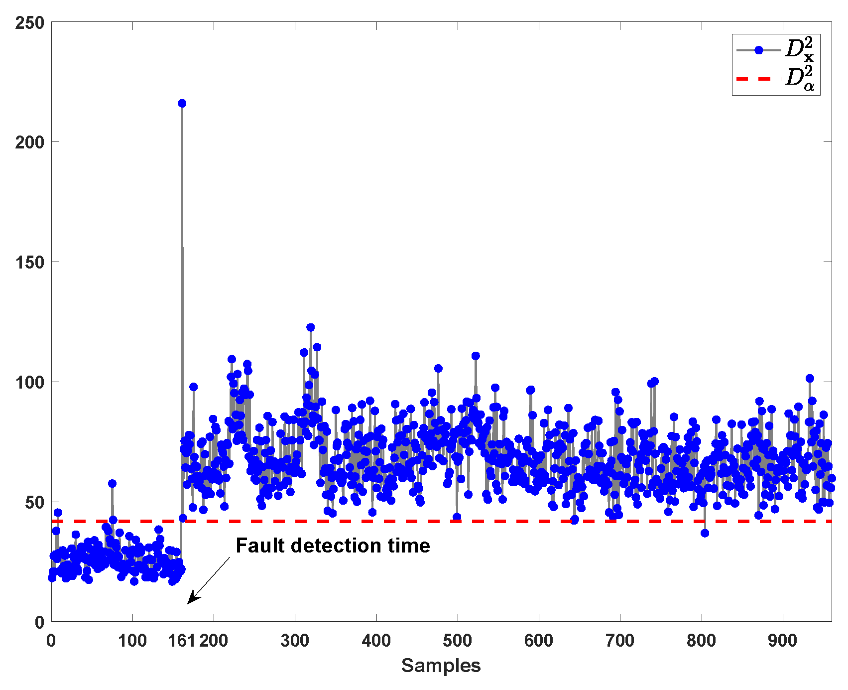
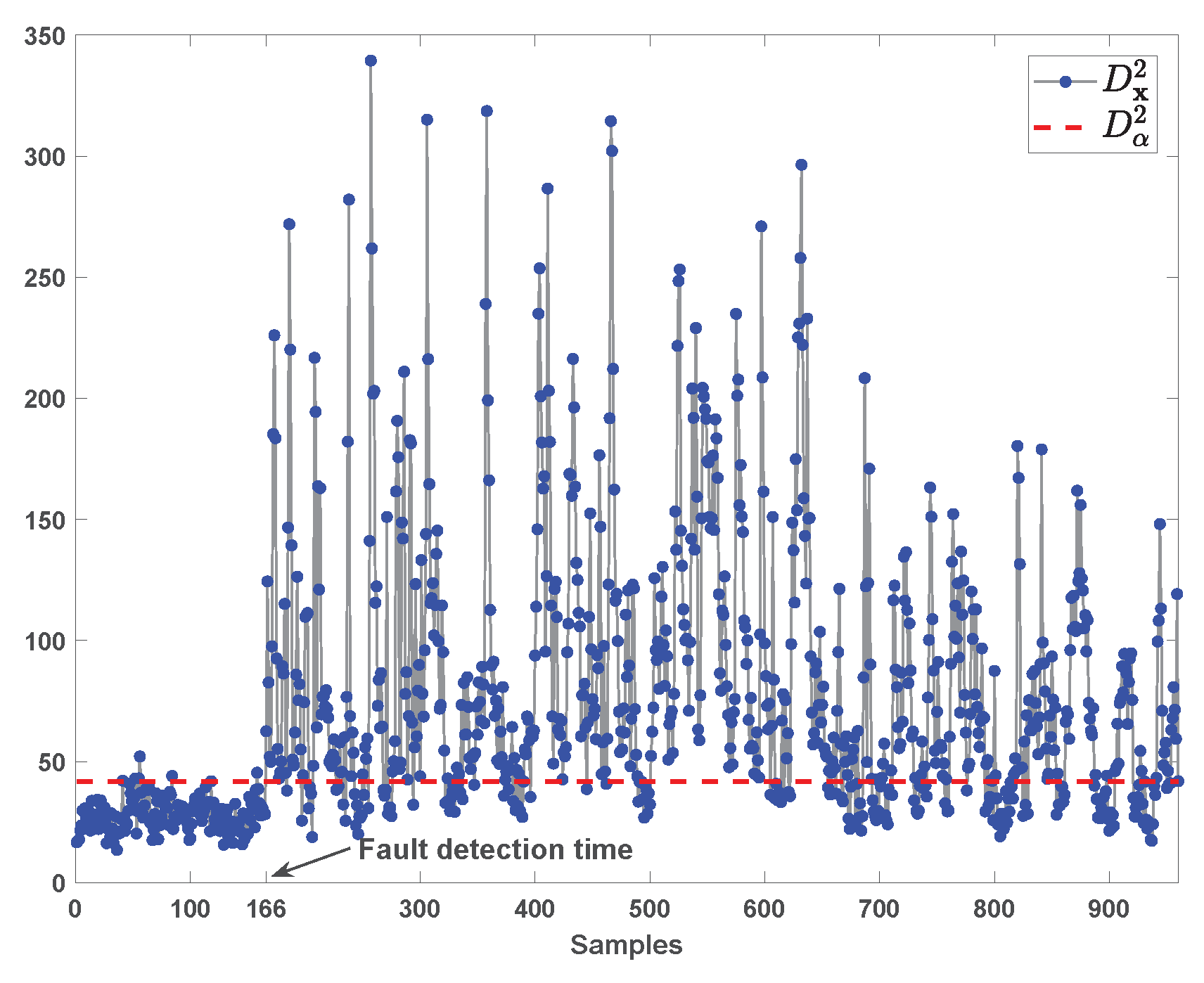
The fault 4 involves a step change in the Reactor Cooling Water Inlet Temperature (unmeasured) [33]. This fault induces a step change in the reactor cooling water flow rate (i.e., variable no.32). When the fault occurs, there is a sudden temperature increase in the reactor (i.e., variable no.9) at 161st sample, which is compensated by the control loops [33].
The monitoring result of fault 4 by kNN is shown in Figure 11. It can be seen that this fault is promptly detected at the 161st sample.
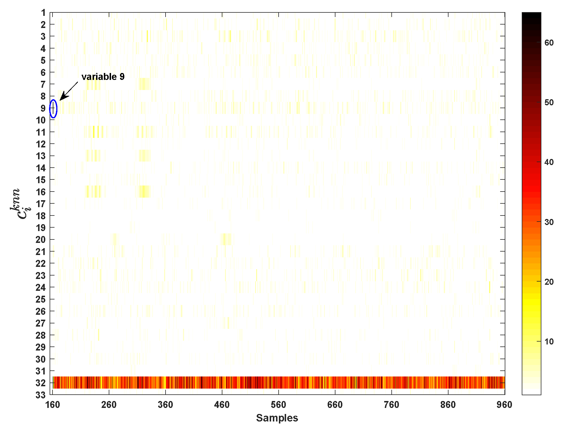
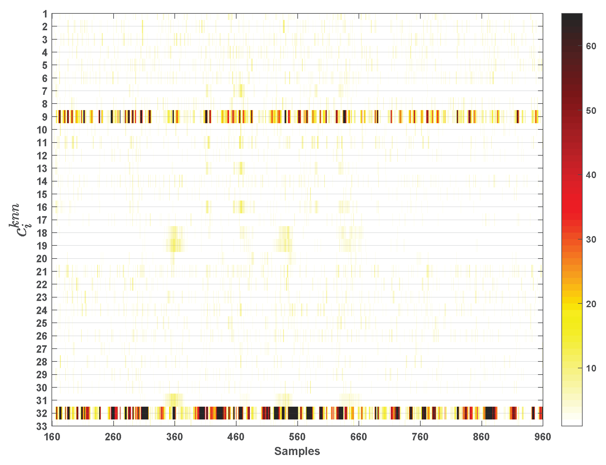
The VCkNN of each variable is shown in Figure 12. The contribution of each variable to the fault from the 161st sample to 960th sample is depicted by color map. The darker the color, the larger the variable contribution; and vice versa. It can be seen that the variable 9 () and 32 () have very large contribution (i.e., black) at 161st sample in Figure 12. After that, the impact of this fault on variable 32 persist.
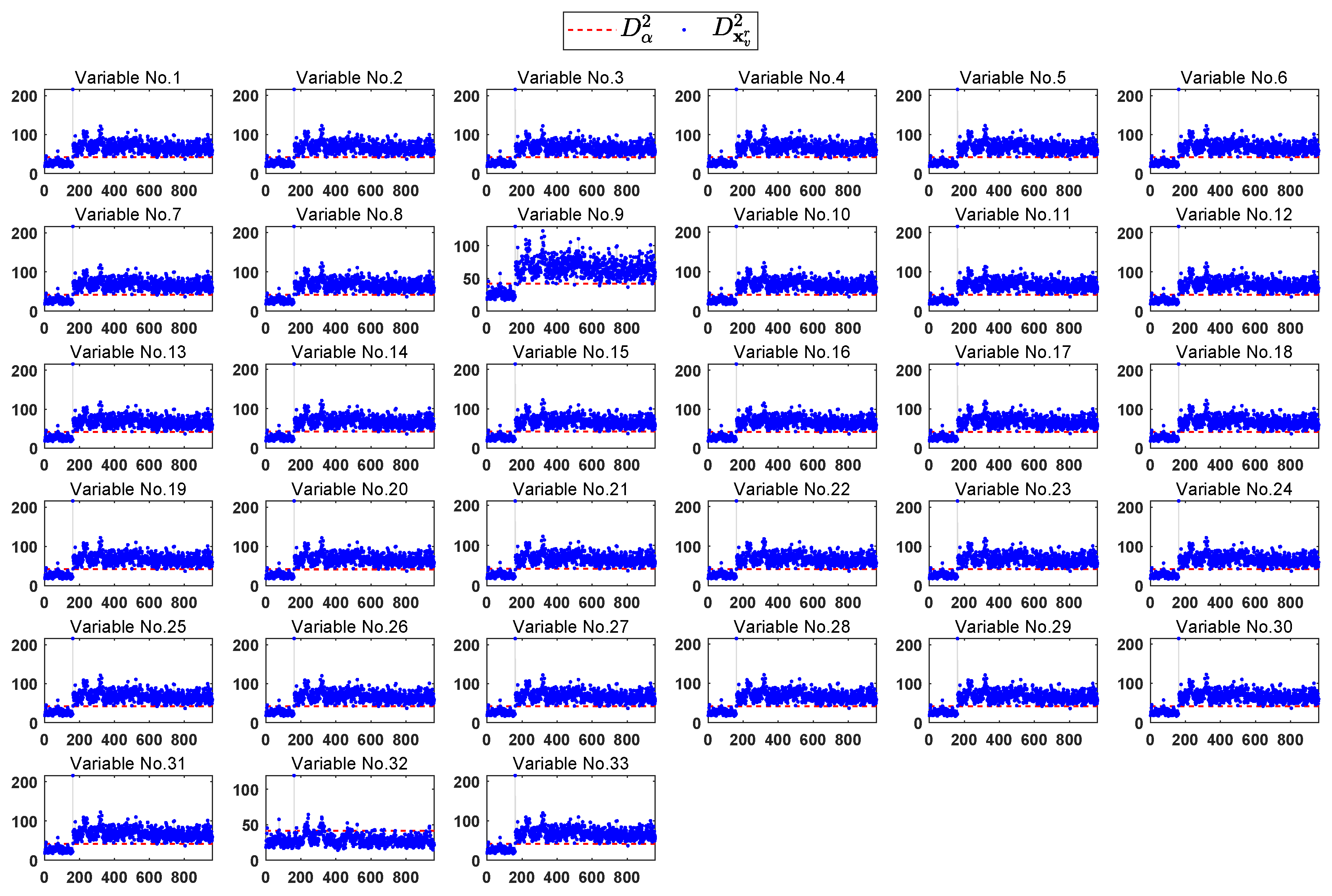
According to the FVI-kNN [28], each variable should be estimated and used in the reconstruction of fault sample. The monitoring results of the reconstruction samples for each variable are shown in Figure 13. It can be seen that most of the fault samples can be brought back to the normal region after eliminating the effect of variable 32.
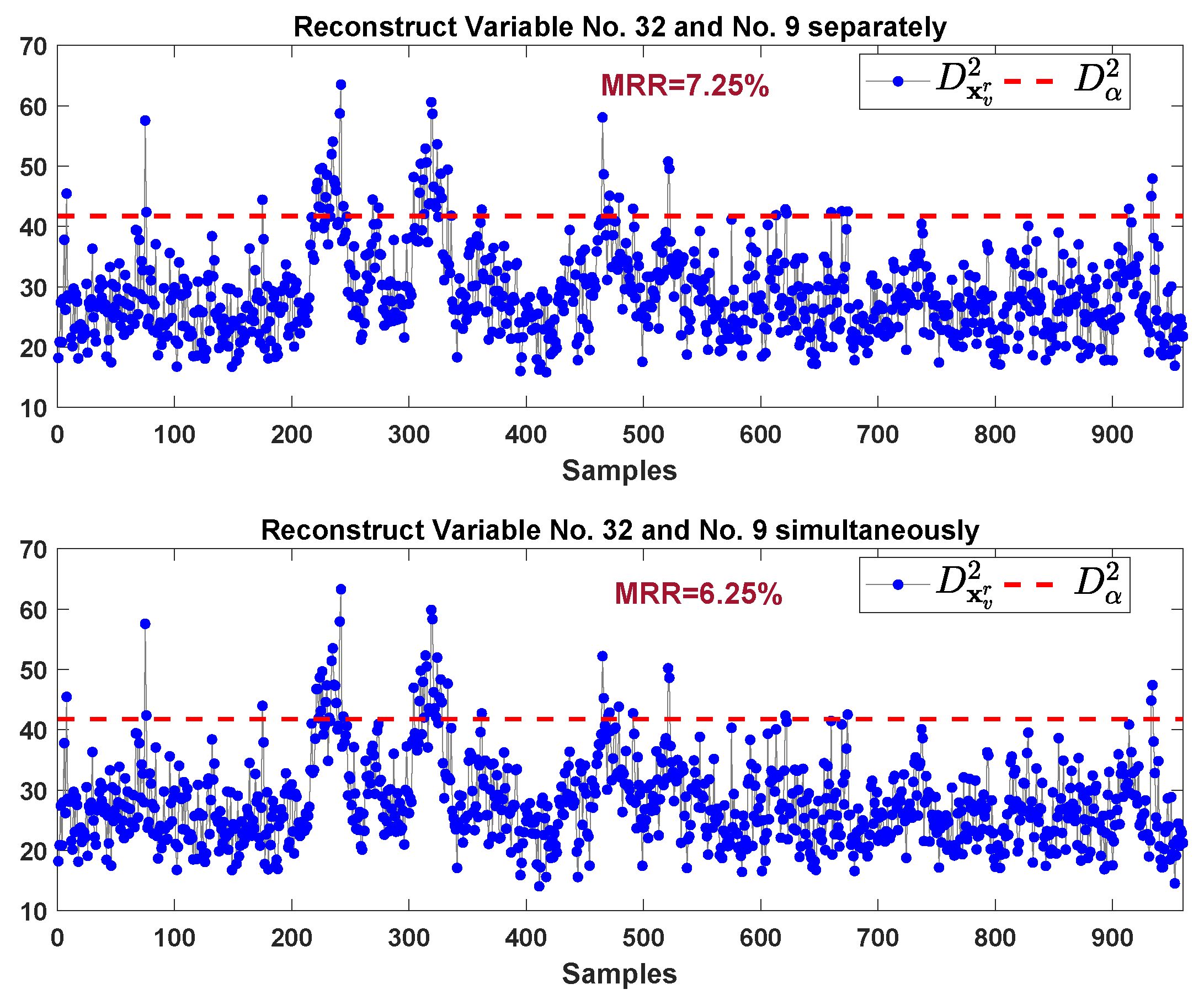
To further consider eliminating effect of variable 32 and 9 on fault samples, the monitoring results of these reconstructed samples are shown in Figure 14. The upper sub-graph of Figure 14 is the monitoring results of reconstruction samples by estimating and replacing variable 32 and 9 separately. Our proposed method provide the monitoring results is shown in the lower sub-graph of Figure 14, where the reconstruction samples is obtained by estimating and replacing variable 32 and 9 simultaneously. Our proposed method gives lower MRR (6.25% vs. 7.25%) compared to the method in Ref. [28].
In this case, our proposed method needs two monitoring charts (i.e., the sub-graph in row 6, column 2 of Figure 13 and lower sub-graph of Figure 14) to correctly identify the faulty variables. On the contrary, the FVI-kNN needs at least 34 monitoring charts ( in the worst case) before the fault variables can be identified. Hence, the proposed method significantly increases the efficiency of the identification procedure.
Fault 11
Similar to fault 4, the fault 11 induces random variation in the reactor cooling water inlet temperature [33]. The fault causes large oscillations in the reactor cooling water flow rate (i.e., variable 32), which results in a fluctuation of reactor temperature (i.e., variable 9). The other 31 variables remain around the set-points and behave similarly as in the NOC [33].
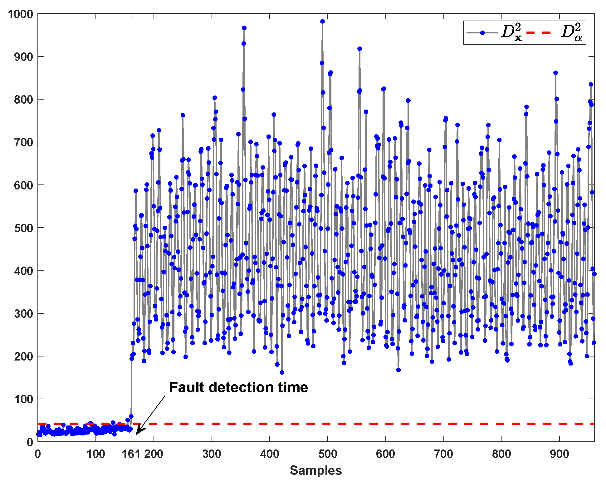
The monitoring result of fault 11 by kNN is shown in Figure 15. It can be seen that this fault is detected at the 166th sample.
The VCkNN of each variable to the fault from the 161st sample to 960th sample is shown in Figure 16. It can be seen that the contribution of variable 9 and 32 to the fault is larger than that of the other variables.
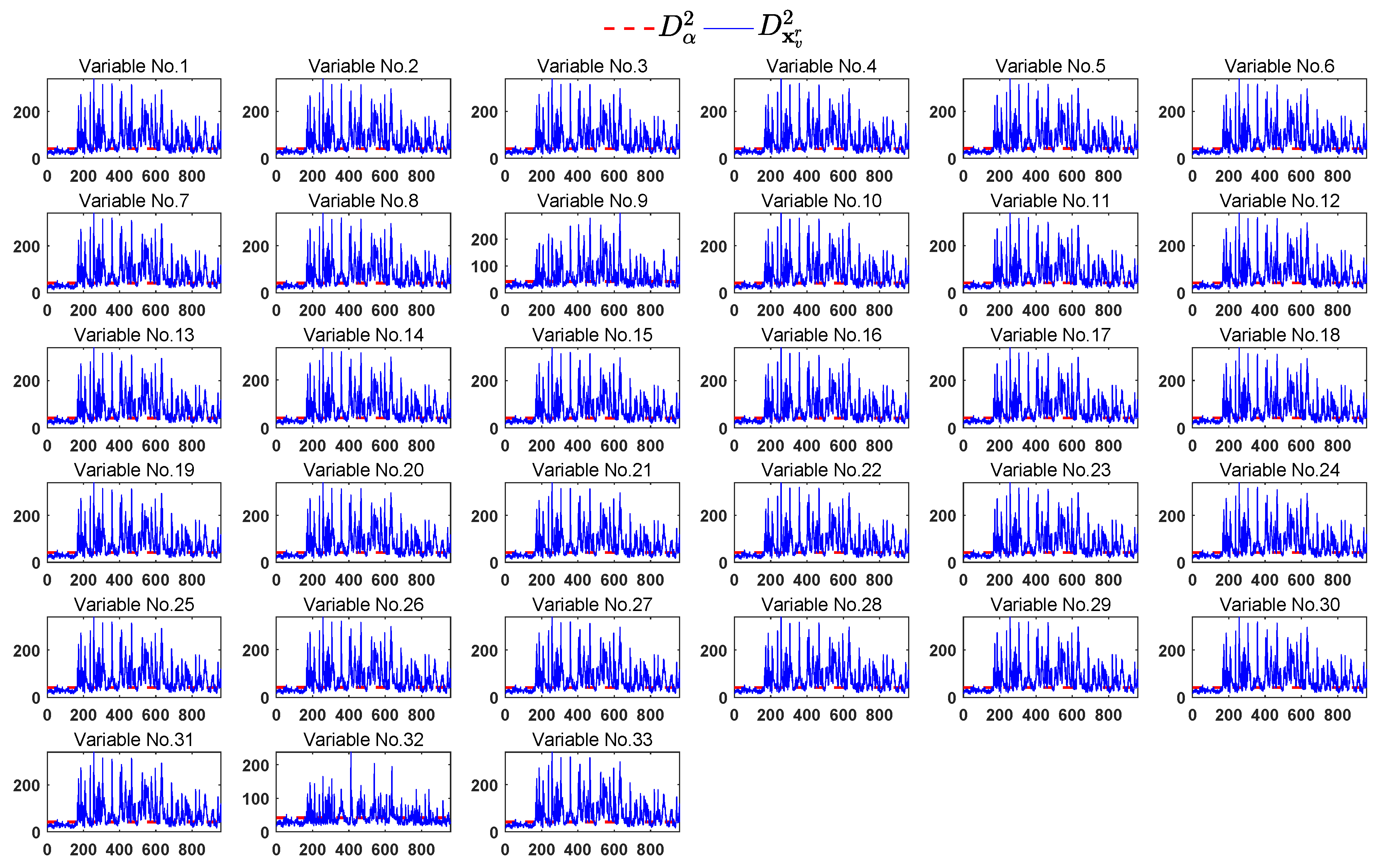
The monitoring results of the reconstruction samples for each variable are shown in Figure 17. It can be seen that most of the fault samples cannot be brought back to the normal region after eliminating the effect of only a single variable. This implies that the fault may affect more than one variable.
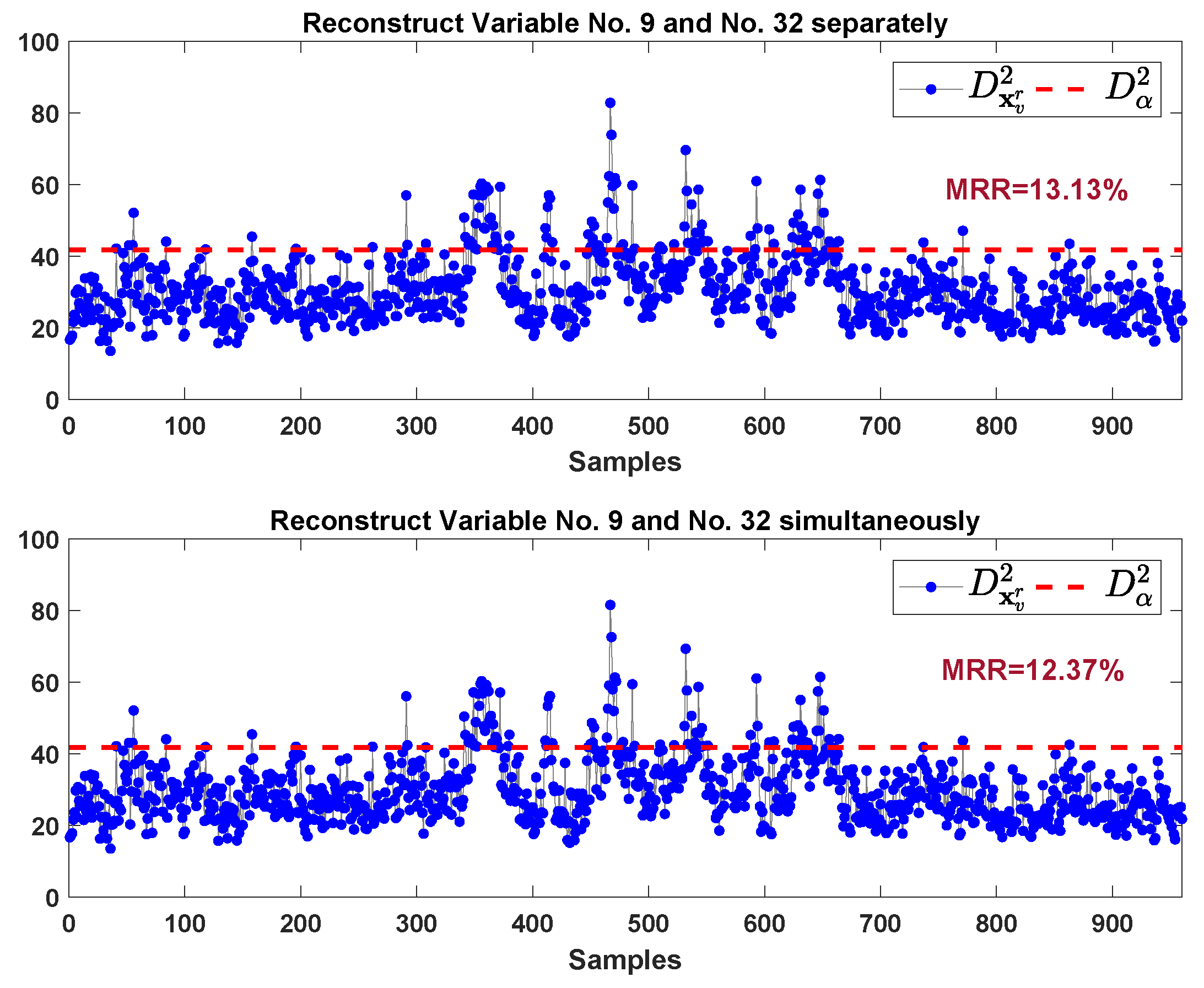
We continue the procedure of reconstruction by considering variable 32 and variable 9. The monitoring results are shown in Figure 18. The upper sub-graph of Figure 18 shows the monitoring results of reconstruction samples by estimating and replacing variable 32 and 9 separately. Our proposed method provide the monitoring results in the lower sub-graph of Figure 18, where the reconstruction samples is obtained by estimating and replacing variable 32 and 9 simultaneously. Our proposed method gives lower MRR (12.37% vs. 13.13%) compared to the method in Ref. [28].
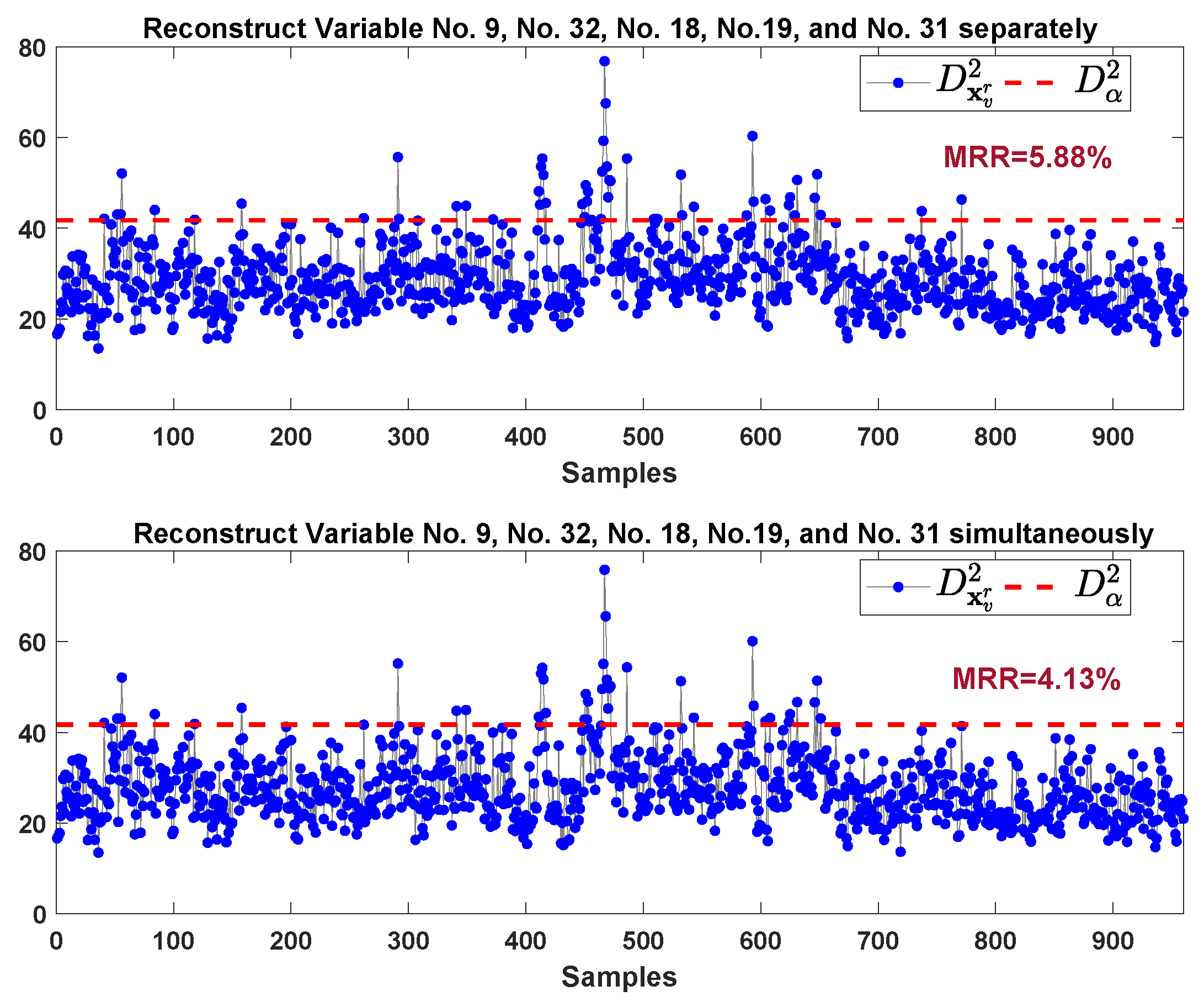
From Figure 18, both methods provide MRR larger than 10% which is not a very satisfied reconstruction result. To further improve MRR, by inspecting VCkNN plot in Figure 16, beside variable 32 and variable 9, the contribution of variable 18, variable 19, and variable 31 are relatively large. After constructing these five variables, the monitoring results are shown in Figure 19. We can see that the MRRs are improved after eliminating more potential faulty variables. Our proposed method can still give lower MRR (4.13% vs. 5.88%) compared to the method in Ref. [28].
Fault 14
The fault 14 induces sticking in Reactor Cooling Water Valve. This fault will affect the reactor cooling water flow (i.e., variable 32), reactor temperature (i.e., variable 9), and reactor cooling water outlet temperature (i.e., variable 21). The monitoring results of fault 11 by kNN is shown in Figure 20. It can be seen that this fault is detected at the 161st sample.
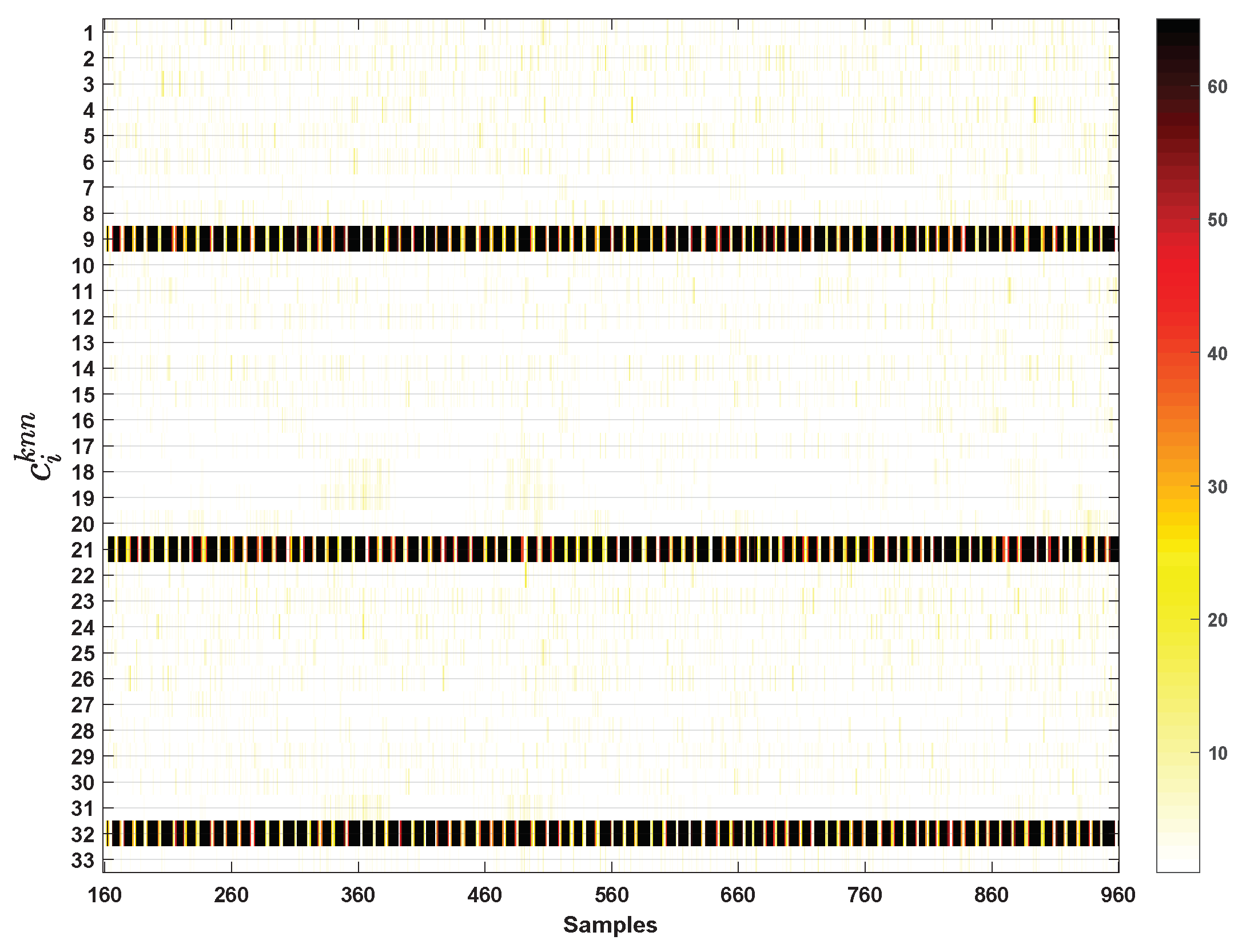
The contribution of each variable to fault 11 from the 161st sample to 960th sample is shown in Figure 21. It can be seen that the contribution of 32, variable 9, and variable 21 to this fault is significantly larger than that of the rest of the variables.
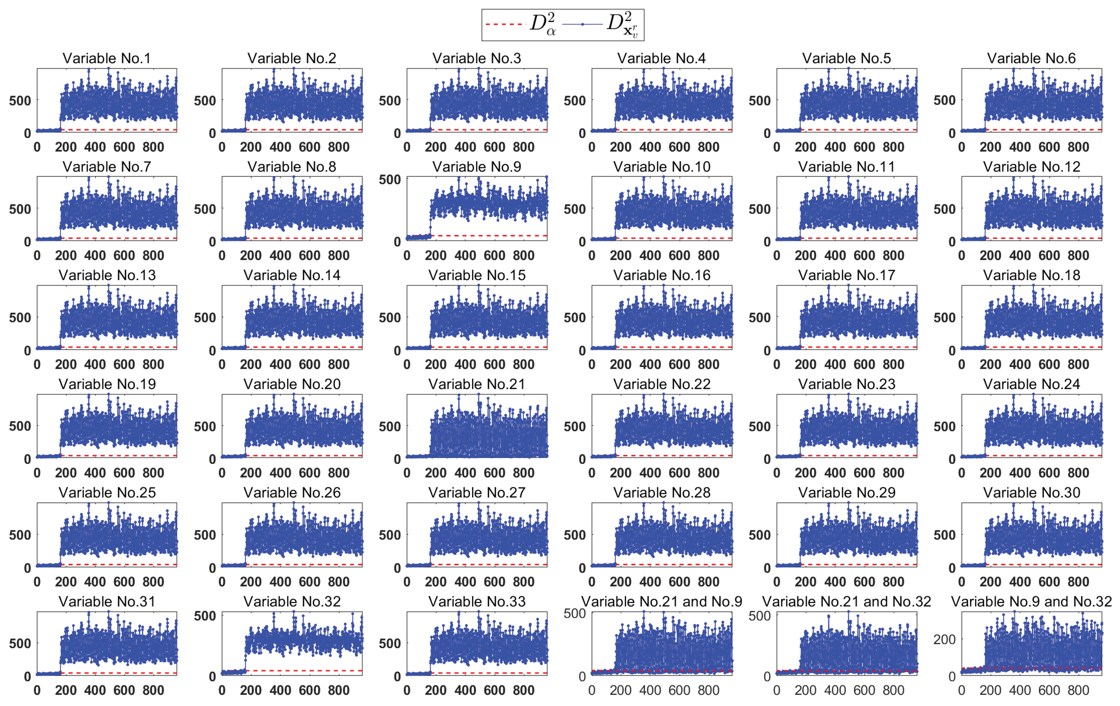
The monitoring results of the reconstruction samples for each variable are shown in the first 33 sub-graphs of Figure 22. It can be seen that most of the fault samples cannot be brought back to the normal region after eliminating the effect of only a single variable. This implies that the fault may affect more than one variable. To continue the reconstruction by exhausting all the combination of any two variables, the results still cannot identify the true faulty variables by FVI-kNN.
In the last three sub-graphs (6th row, last three columns) of Figure 22, we provide the monitoring results of the reconstruction samples by separately eliminating and replacing any two among variable 9, variable 32, and variable 21. Obviously, the fault samples still cannot be brought back to the normal region.
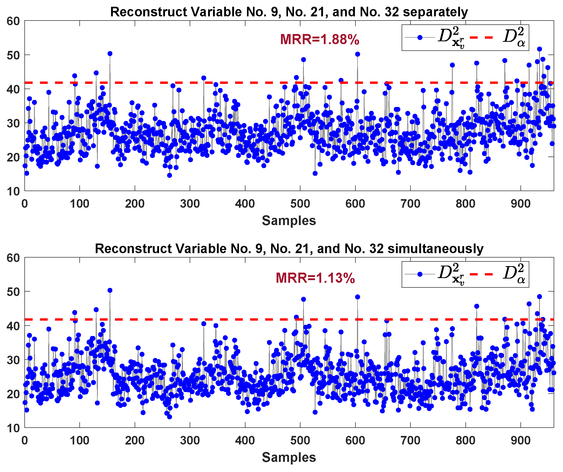
We continue the procedure of the fault sample reconstruction by considering variable 32, variable 9, and variable 21. The monitoring results are shown in Figure 23. The upper sub-graph of Figure 23 is the monitoring results of the reconstruction samples by estimating and replacing these three variables separately. Our proposed method provides the monitoring results in the lower sub-graph of Figure 18, where the reconstruction samples are obtained by estimating and replacing these three variables simultaneously. Our proposed method gives lower MRR (1.13% vs. 1.88%) compared to the FVI-kNN. In addition, our proposed method needs three reconstruction monitoring charts while the FVI-kNN needs at least monitoring charts ( in the worst case) before the faulty variables can be identified. Hence, this again demonstrates the superior of the proposed method in the efficiency of the identification procedure.
Table 2 summarizes the results of the three faults of TEP. It can be seen that our proposed method always provides lower MRR while only needs extremely few reconstruction times compared with FVI-kNN.
5. Discussion
For fault detection, the comparison between PCA and kNN has been demonstrated by several studies [7,15,35]. For fault identification/isolation, more specifically in the frame of MSPM, the contribution plot, FDA, and their variants are commonly used methods. Compared with contribution plot, the proposed method improves the identification accuracy by using the VCkNN, which does not suffer from smearing effect and has been proven to have the ability to give more accurate results of variable contribution. However, this build-in advantage, due to the smearing effect, cannot be found in the contribution plot/contribution analysis methods. Therefore, the unreliable ranking of variable contribution provided by contribution plot will reduce the accuracy of the FDI results. The FDA needs fault information such as fault direction (difficult to obtain) to conduct fault isolation/diagnosis [35] while our proposed method identifies the faulty variables by using only the NOC data.
In the case of multiple faulty variables, FVI-kNN still reconstructs the fault sample by replacing the possible faulty variables obtained in the estimation of single variable. This estimation of single variable is inaccurate when there are multiple faulty variables. This is illustrated by the case 2 of numerical simulation. When the magnitude of the step fault is large, the FVI-kNN’s inaccurate estimations of possible faulty variables produce very high missing reconstruction ratio. In contrast, the proposed method simultaneously estimates the possible faulty variables and guarantees the replaced variables used in reconstruction samples are accurate. This leads to an acceptable missing reconstruction ratio.
It worth noting that the proposed method needs VCkNN to guide the variable selection for the reconstruction procedure. The underlying assumption of VCkNN is that the fault magnitude is significantly larger than the distance between the fault sample and its k-nearest neighbors [19]. If this assumption is satisfied, the VCkNN ensures that the contributions of the faulty variables are always larger than that of non-faulty variables. Otherwise, there is no guarantee that the ranking of the variable contributions can be provided by VCkNN.
Furthermore, the kNN reconstruction uses the non-faulty variables to estimate the possible faulty variables. When a fault affects most of the variables, the kNN regression may be difficult to provide accurate estimation based on only few non-faulty variables. In this situation, the proposed method may also be difficult to give reliable identification for faulty variables. These problems need further investigation.
6. Conclusions
In this work, we develop an efficient method by fas kNN reconstruction for identifying the faulty variables in the process industry. The VCkNN is used to guide the variable selection in the identification procedure. The proposed method can not only significantly reduce the computation time of identification procedure, but also produce a lower missing reconstruction ratio compared to the existing kNN-based reconstruction methods. The numerical simulation and TE process experiments demonstrate the effectiveness of our presented method.
Author Contributions
Z.Z., Z.L., P.W. conceived and designed the method and wrote the paper. Z.Z., Z.C. performed the experiments.
Funding
This research was funded by NATIONAL NATURAL SCIENCE FOUNDATION OF CHINA grant number 61703158, 61573136, 61573137 and ZHEJIANG PROVINCIAL PUBLIC WELFARE TECHNOLOGY RESEARCH PROJECT grant number 2016C31115, LGG19F030009 and SCIENTIFIC RESEARCH PROJECT OF HUZHOU UNIVERSITY grand number 2017XJXM36, 2018XJKJ50.
Conflicts of Interest
The authors declare no conflict of interest. The funders had no role in the design of the study; in the collection, analyses, or interpretation of data; in the writing of the manuscript, or in the decision to publish the results.
Abbreviations
The following abbreviations are used in this manuscript:
| kNN | k Nearest Neighbor |
| VCkNN | Variable Contribution by kNN |
| MSPM | Multivariate Statistical Process Monitoring |
| FD-kNN | Fault Detection based on kNN |
| NOC | Normal Operation Condition |
| FVI-kNN | Fault Variable Identification based on kNN |
| MRI | Maximum Reduction In Detection Index |
| IFVI-kNN | Improved FVI-kNN |
| MRR | Missing Reconstruction Ratio |
| TE | Tennessee Eastman |
References
- He, Q.P.; Wang, J.; Shah, D. Feature Space Monitoring for Smart Manufacturing via Statistics Pattern Analysis. Comput. Chem. Eng. 2019. [Google Scholar] [CrossRef]
- Ge, Z.; Song, Z.; Ding, S.X.; Huang, B. Data Mining and Analytics in the Process Industry: The Role of Machine Learning. IEEE Access 2017, 5, 20590–20616. [Google Scholar] [CrossRef]
- Ge, Z. Review on data-driven modeling and monitoring for plant-wide industrial processes. Chemom. Intell. Lab. Syst. 2017, 171, 16–25. [Google Scholar] [CrossRef]
- Qin, S.J. Survey on data-driven industrial process monitoring and diagnosis. Annu. Rev. Control 2012, 36, 220–234. [Google Scholar] [CrossRef]
- Ge, Z.; Song, Z.; Gao, F. Review of recent research on data-based process monitoring. Ind. Eng. Chem. Res. 2013, 52, 3543–3562. [Google Scholar] [CrossRef]
- Yin, S.; Ding, S.; Xie, X.; Luo, H. A Review on Basic Data-Driven Approaches for Industrial Process Monitoring. IEEE Trans. Ind. Electron. 2014, 61, 6418–6428. [Google Scholar] [CrossRef]
- He, Q.P.; Wang, J. Fault detection using the k-nearest neighbor rule for semiconductor manufacturing processes. IEEE Trans. Semicond. Manuf. 2007, 20, 345–354. [Google Scholar] [CrossRef]
- Zhao, S.; Zhang, J.; Xu, Y. Monitoring of processes with multiple operating modes through multiple principle component analysis models. Ind. Eng. Chem. Res. 2004, 43, 7025–7035. [Google Scholar] [CrossRef]
- Qin, Y.; Zhao, C.; Zhang, S.; Gao, F. Multimode and Multiphase Batch Processes Understanding and Monitoring Based on between-Mode Similarity Evaluation and Multimode Discriminative Information Analysis. Ind. Eng. Chem. Res. 2017, 56, 9679–9690. [Google Scholar] [CrossRef]
- Zhang, S.; Zhao, C.; Gao, F. Two-directional concurrent strategy of mode identification and sequential phase division for multimode and multiphase batch process monitoring with uneven lengths. Chem. Eng. Sci. 2018, 178, 104–117. [Google Scholar] [CrossRef]
- Lee, J.M.; Yoo, C.; Choi, S.W.; Vanrolleghem, P.A.; Lee, I.B. Nonlinear process monitoring using kernel principal component analysis. Chem. Eng. Sci. 2004, 59, 223–234. [Google Scholar] [CrossRef]
- Ge, Z.; Song, Z. Process monitoring based on independent component analysis-principal component analysis (ICA-PCA) and similarity factors. Ind. Eng. Chem. Res. 2007, 46, 2054–2063. [Google Scholar] [CrossRef]
- Yu, W.; Zhao, C. Robust Monitoring and Fault Isolation of Nonlinear Industrial Processes Using Denoising Autoencoder and Elastic Net. IEEE Trans. Control Syst. Technol. 2019. [Google Scholar] [CrossRef]
- Zhao, C.; Huang, B. A Full-condition Monitoring Method for Nonstationary Dynamic Chemical Processes with Cointegration and Slow Feature Analysis. AIChE J. 2018, 64, 1662–1681. [Google Scholar] [CrossRef]
- He, Q.P.; Wang, J. Large-scale semiconductor process fault detection using a fast pattern recognition-based method. IEEE Trans. Semicond. Manuf. 2010, 23, 194–200. [Google Scholar] [CrossRef]
- Verdier, G.; Ferreira, A. Adaptive Mahalanobis Distance and k-Nearest Neighbor Rule for Fault Detection in Semiconductor Manufacturing. IEEE Trans. Semicond. Manuf. 2011, 24, 59–68. [Google Scholar] [CrossRef]
- Li, Y.; Zhang, X. Diffusion maps based k-nearest-neighbor rule technique for semiconductor manufacturing process fault detection. Chemom. Intell. Lab. Syst. 2014, 136, 47–57. [Google Scholar] [CrossRef]
- Zhou, Z.; Wen, C.L.; Yang, C.J. Fault Detection Using Random Projections and k-Nearest Neighbor Rule for Semiconductor Manufacturing Processes. IEEE Trans. Semicond. Manuf. 2015, 28, 70–79. [Google Scholar] [CrossRef]
- Zhou, Z.; Wen, C.; Yang, C. Fault Isolation Based on k-Nearest Neighbor Rule for Industrial Processes. IEEE Trans. Ind. Electron. 2016, 63, 2578–2586. [Google Scholar] [CrossRef]
- Miller, P.; Swanson, R.E.; Heckler, C.E. Contribution plots: A missing link in multivariate quality control. Appl. Math. Comput. Sci. 1998, 8, 775–792. [Google Scholar]
- Dunia, R.; Qin, S.J.; Edgar, T.F.; McAvoy, T.J. Identification of faulty sensors using principal component analysis. AIChE J. 1996, 42, 2797–2812. [Google Scholar] [CrossRef]
- Yue, H.H.; Qin, S.J. Reconstruction-based fault identification using a combined index. Ind. Eng. Chem. Res. 2001, 40, 4403–4414. [Google Scholar] [CrossRef]
- Alcala, C.F.; Qin, S.J. Reconstruction-based contribution for process monitoring. Automatica 2009, 45, 1593–1600. [Google Scholar] [CrossRef]
- Alcala, C.F.; Qin, S.J. Analysis and generalization of fault diagnosis methods for process monitoring. J. Process Control 2011, 21, 322–330. [Google Scholar] [CrossRef]
- Westerhuis, J.A.; Gurden, S.P.; Smilde, A.K. Generalized contribution plots in multivariate statistical process monitoring. Chemom. Intell. Lab. Syst. 2000, 51, 95–114. [Google Scholar] [CrossRef]
- Mnassri, B.; Adel, E.; Mostafa, E.; Ouladsine, M. Generalization and analysis of sufficient conditions for PCA-based fault detectability and isolability. Annu. Rev. Control 2013, 37, 154–162. [Google Scholar] [CrossRef]
- Mnassri, B.; Adel, E.M.E.; Ouladsine, M. Reconstruction-based Contribution approaches for improved fault diagnosis using principal component analysis. J. Process Control 2015, 33, 60–76. [Google Scholar] [CrossRef]
- Wang, G.; Liu, J.; Li, Y. Fault diagnosis using kNN reconstruction on MRI variables. J. Chemom. 2015, 29, 399–410. [Google Scholar] [CrossRef]
- Zhou, Z.; Lei, J.; Ge, Z.; Xu, X. Fault variables recognition using improved k-nearest neighbor reconstruction. In Proceedings of the 2017 Chinese Automation Congress (CAC), Jinan, China, 20–22 October 2017; pp. 5562–5565. [Google Scholar] [CrossRef]
- He, B.; Yang, X.; Chen, T.; Zhang, J. Reconstruction-based multivariate contribution analysis for fault isolation: A branch and bound approach. J. Process Control 2012, 22, 1228–1236. [Google Scholar] [CrossRef] [Green Version]
- Zhao, C.; Wang, W. Efficient faulty variable selection and parsimonious reconstruction modelling for fault isolation. J. Process Control 2016, 38, 31–41. [Google Scholar] [CrossRef]
- Downs, J.J.; Vogel, E.F. A plant-wide industrial process control problem. Comput. Chem. Eng. 1993, 17, 245–255. [Google Scholar] [CrossRef]
- Russell, E.L.; Chiang, L.H.; Braatz, R.D. Data-Driven Techniques for Fault Detection and Diagnosis in Chemical Processes; Springer: London, UK, 2000. [Google Scholar] [CrossRef]
- Russell, E.; Chiang, L.; Braatz, R. Tennessee Eastman Problem Simulation Data. Available online: http://web.mit.edu/braatzgroup/links.html (accessed on 27 April 2015).
- He, Q.P.; Qin, S.J.; Wang, J. A new fault diagnosis method using fault directions in Fisher discriminant analysis. AIChE J. 2005, 51, 555–571. [Google Scholar] [CrossRef]
Figure 1.
The flowchart of fault sample reconstruction by k-nearest neighbor (kNN) estimation.

Figure 2.
The fault detection results based on kNN for case 1 of numerical simulation.

Figure 3.
The fault detection results by eliminating faulty variables for case 1.

Figure 4.
The variable contribution by kNN for case 1 of numerical simulation.

Figure 5.
The fault detection results based on kNN for case 2 of numerical simulation.

Figure 6.
The variable contribution by kNN for case 2 of numerical simulation.

Figure 7.
The fault detection results by eliminating faulty variable for case 2.

Figure 8.
The fault detection results based on kNN for case 3 of numerical simulation.

Figure 9.
The variable contribution by kNN for case 3 of numerical simulation.

Figure 10.
The fault detection results by eliminating faulty variable for case 3.

Figure 11.
The fault detection results by kNN for fault 4 of Tennessee Eastman (TE).

Figure 12.
The variable contribution by kNN for fault 4 of TE.

Figure 13.
The fault detection results of reconstructed samples by estimating and replacing each variable for fault 4 of TE.
Figure 13.
The fault detection results of reconstructed samples by estimating and replacing each variable for fault 4 of TE.

Figure 14.
The fault detection results of reconstructed samples by estimating and replacing variable No.32 and No.9 for fault 4 of TE.
Figure 14.
The fault detection results of reconstructed samples by estimating and replacing variable No.32 and No.9 for fault 4 of TE.

Figure 15.
The fault detection results by kNN for fault 11 of TE.

Figure 16.
The variable contribution by kNN for fault 11 of TE.

Figure 17.
The fault detection results of reconstructed samples by estimating and replacing each variable for fault 11 of TE.
Figure 17.
The fault detection results of reconstructed samples by estimating and replacing each variable for fault 11 of TE.

Figure 18.
The fault detection results of reconstructed samples by estimating and replacing variable No.32 and No.9 for fault 11 of TE.
Figure 18.
The fault detection results of reconstructed samples by estimating and replacing variable No.32 and No.9 for fault 11 of TE.

Figure 19.
The fault detection results of reconstructed samples by estimating and replacing variable No.32, No.9, No.18, No.19, and No.31 (with larger VCkNN) for fault 11 of TE.
Figure 19.
The fault detection results of reconstructed samples by estimating and replacing variable No.32, No.9, No.18, No.19, and No.31 (with larger VCkNN) for fault 11 of TE.

Figure 20.
The fault detection results by kNN for fault 14 of TE.

Figure 21.
The variable contribution by kNN for fault 14 of TE.

Figure 22.
The fault detection results of reconstructed samples by estimating and replacing each variable for fault 14 of TE.
Figure 22.
The fault detection results of reconstructed samples by estimating and replacing each variable for fault 14 of TE.

Figure 23.
The fault detection results of reconstructed samples by estimating and replacing variable No.9, No.21, and No.32 for fault 14 of TE.
Figure 23.
The fault detection results of reconstructed samples by estimating and replacing variable No.9, No.21, and No.32 for fault 14 of TE.


Table 1.
The summarized results of the numerical case study.
| Cases | Fault Detection Time | MRR(%) | Reconstruction Times Required | ||
|---|---|---|---|---|---|
| FVI-kNN | Proposed Method | FVI-kNN | Proposed Method | ||
| case 1 | 301st | 2.5 | 0.5 | 8(28) a | 2 |
| case 2 | 301st | 69 | 0.5 | 8(28) | 2 |
| case 3 | 326th | 25 | 0.5 | 8(28) | 2 |
a A(B) A is the minimum times of reconstruction required; B is maximum times of reconstruction required.
Table 2.
The summarized results of the three faults on TEP.
| Faults | Fault Detection Time | MRR(%) | Reconstruction Times Required | ||
|---|---|---|---|---|---|
| FVI-kNN | Proposed Method | FVI-kNN | Proposed Method | ||
| Fault 1 | 161st | 7.25 | 6.25 | 34(528) a | 2 |
| Fault 11 | 166th | 5.88 | 4.13 | 40,922(237,336) | 5 |
| Fault 14 | 161st | 1.88 | 1.13 | 529(5456) | 3 |
a A(B) A is the minimum times of reconstruction required; B is maximum times of reconstruction required.
© 2019 by the authors. Licensee MDPI, Basel, Switzerland. This article is an open access article distributed under the terms and conditions of the Creative Commons Attribution (CC BY) license (http://creativecommons.org/licenses/by/4.0/).
Share and Cite
MDPI and ACS Style
Zhou, Z.; Li, Z.; Cai, Z.; Wang, P. Fault Identification Using Fast k-Nearest Neighbor Reconstruction. Processes 2019, 7, 340. https://doi.org/10.3390/pr7060340
AMA Style
Zhou Z, Li Z, Cai Z, Wang P. Fault Identification Using Fast k-Nearest Neighbor Reconstruction. Processes. 2019; 7(6):340. https://doi.org/10.3390/pr7060340
Chicago/Turabian StyleZhou, Zhe, Zuxin Li, Zhiduan Cai, and Peiliang Wang. 2019. "Fault Identification Using Fast k-Nearest Neighbor Reconstruction" Processes 7, no. 6: 340. https://doi.org/10.3390/pr7060340
Note that from the first issue of 2016, this journal uses article numbers instead of page numbers. See further details here.