Parallel Implementation of the Deterministic Ensemble Kalman Filter for Reservoir History Matching

Abstract

In this paper, the deterministic ensemble Kalman filter is implemented with a parallel technique of the message passing interface based on our in-house black oil simulator. The implementation is separated into two cases: (1) the ensemble size is greater than the processor number and (2) the ensemble size is smaller than or equal to the processor number. Numerical experiments for estimations of three-phase relative permeabilities represented by power-law models with both known endpoints and unknown endpoints are presented. It is shown that with known endpoints, good estimations can be obtained. With unknown endpoints, good estimations can still be obtained using more observations and a larger ensemble size. Computational time is reported to show that the run time is greatly reduced with more CPU cores. The MPI speedup is over 70% for a small ensemble size and 77% for a large ensemble size with up to 640 CPU cores.

1. Introduction

The ensemble Kalman filter (EnKF) is a data assimilation method to estimate poorly known model solutions and/or parameters by integrating the given observation data. It was introduced by Evensen [1] and has attracted a lot of attention in the fields of weather forecasting sciences, oceanographic sciences and reservoir engineering. Regarded as a Monte Carlo formulation of the Kalman Filter, it is applied to each ensemble forecast in an analysis step. The deterministic ensemble Kalman filter (DEnKF) is a variation of the EnKF which has an asymptotic match of the analysis error covariance from the Kalman filter theory with a small correction and without any perturbed observation; its form is simpler while its robust property is still kept [2].

The EnKF has been introduced to reservoir engineering in the past decade. As a data assimilation method for history matching, the EnKF can be used to assimilate different kinds of production data, estimate model parameters and adjust dynamical variables. It was first applied to history matching by Nævdal [3,4]. A detailed review was given by Aanonsen et al. [5]. It has been used to estimate reservoir porosity and permeability successfully [4,6,7]. It has also been adopted to estimate relative permeability and capillary pressure curves with good accuracy [8,9,10,11]. Nevertheless, for most of the applications, hundreds of the ensemble members are required to guarantee the accuracy of an estimation. For example, an estimation of endpoints of relative permeability curves is challenging; a good estimation can only be obtained in limited cases [8,9] and requires a large ensemble size. Therefore, a serial run of simulations is very time-consuming. Furthermore, for large-scale numerical models, the memory of one single processor may even not be enough for a simulation with one ensemble member. Therefore, the parallel technique becomes a natural choice to reduce the computational time and make large-scale models feasible.

The parallel technique has been successfully applied in many fields including atmosphere and oceanographic sciences. A multivariate ensemble Kalman filter was implemented on a massively parallel computer architecture for the Poseidon ocean circulation model [12]. At an EnKF forecast step, each ensemble member is distributed to a different processor. To parallelize an analysis step, the ensemble is transposed over processors according to domain decomposition. A parallelized localization implementation was reported in [13] based on domain decomposition. As for the reservoir history matching, the parallel technique has not been well developed. An automatic history matching module with distributed and parallel computing was done by Liang et al. using weigthed EnKF [14], where two-level high-performance computing is implemented, distributing ensemble members simultaneously by submitting all the simulation jobs at the same time and simulating each ensemble member in parallel. A parallel framework was given by Tavakoli et al. [15] using the EnkF and ensemble smoother (ES) methods based on the simulator IPARS, in which a forecast step was parallelized while an analysis step was computed by one central processor. It discussed the case where the processor number is fewer than the ensemble size and each processor is in charge of one or several ensemble members according to its simulation speed. In their another work [16], the case where the processor number is greater than the ensemble size was also discussed. For parallelizing an analysis step, the parallelization was carried out by partitioning a matrix in a row-wise manner. Comparing to the EnKF, ES requires less time to assimilating the data as it does not need to synchronize all the ensemble members at the analysis step. However, for the large data point problems, the matrices become very large, resulting in long computational time and large memory requirements for the inversion.

Although the implementation of the parallel technique was explored in the above papers, good computational efficiency has not been obtained, even with high performance simulators. One important reason is that after each analysis step, updated variable values were written on a disk and read by different processors to restart a simulator. A large number of inputs/outputs not only waste the disk space, but also slow down accessing, reading and writing. On the other hand, an analysis step must have been done after all the simulations in a forecast step are finished. This synchronization determines that at every forecast step, the simulation time equals the maximum run time among all the processors. From the parallel aspect, MPI inputs/outputs have poor performance on common computer clusters. Load and storage operations are more time-consuming than multiplication operations. Moreover, parallelization of an analysis step needs message passing multiple times. According to the above published papers, the parallel efficiency was generally lower than 50% with an ensemble of no more than 200 members compared to the ideal efficiency 100%.

In contrast to the traditional EnKF method, some modifications of this method have been done and different filters have been developed, such as Ensemble Square Root Filters (ESRFs) [17,18] and deterministic Ensemble Kalman filters (DEnKF) [2] that give better performance in certain conditions. First proposed by Sakov et al. [17], DEnKF can be regarded as a linear approximation to the ESRF under a small analysis correction condition, and it combines the simplicity of the ESRF and the versatility of the traditional EnKF. Its robust property has been shown by numerical experiments [17]. Despite the intensive research and implementation of EnKF, to our knowledge, the DEnKF has not been adopted in the reservoir history matching field yet.

In this paper, the DEnKF is implemented for reservoir history matching with a parallel technique and our in-house parallel black oil simulator. Both forecast and analysis steps are parallelized according to a relationship between an ensemble size and a processor number. To improve the computational efficiency, several switches are defined to control the input/output and set by the user. The restart of the simulator is slightly modified to coordinate the history matching implementation. The simulator is called as a function from our platform library.

This paper is organized as follows. First, our black oil simulator is briefly introduced. After that, the EnKF and DEnKF are given, followed by a parallel technique used in our computations. Based on this technique, numerical experiments on the estimation of relative permeability curves with known endpoints and unknown endpoints are presented. The parallel speedup is reported to show the computational efficiency. Conclusions are given at the end of this paper.

2. Black Oil Simulator

In this paper, a black oil model is simulated. Using the mass conservation law and Darcy’s law on water, oil and gas, the following equations can be obtained [19,20]:

$$\left\{\begin{array}{c}\nabla (\frac{K{K}_{rw}{\rho }_w}{{\mu }_w}\nabla {\mathsf{\Phi }}_w)+q_w=\frac{\partial \left(\varphi {\rho }_w{S}_w\right)}{\partial t}\hfill \\ \nabla (\frac{K{K}_{ro}{\rho }_o^o}{{\mu }_o}\nabla {\mathsf{\Phi }}_o)+q_o=\frac{\partial \left(\varphi {\rho }_o^o{S}_o\right)}{\partial t}\hfill \\ \nabla (\frac{K{K}_{ro}{\rho }_o^g}{{\mu }_o}\nabla {\mathsf{\Phi }}_o)+\nabla (\frac{K{K}_{rg}{\rho }_g^g}{{\mu }_g}\nabla {\mathsf{\Phi }}_g)+q_g\hfill \\ =\frac{\partial \left(\varphi {\rho }_o^g{S}_o\right)}{\partial t}+\frac{\partial \left(\varphi {\rho }_g^g{S}_g\right)}{\partial t}.\hfill \end{array}\right.$$

(1)

In these equations, K is the absolute permeability tensor of a reservoir; $K_{rl}$ and $S_l$ are the relative permeability and saturation of phase l ($l=w,o,g)$, respectively; ${\rho }_w$ is the water density; ${\rho }_o^o$ is the oil component density in the oil phase; ${\rho }_o^g$ is the gas component density in the oil phase; and ${\rho }_g^g$ is the gas component density in the gas phase. The potential of phase l has the form

$${\mathsf{\Phi }}_l=P_l-\mathcal{G}{\rho }_{l}z$$

where $P_l$ is the pressure of phase l ($l=w,o,g)$, $\mathcal{G}$ is the magnitude of the gravitational constant and z is the depth of the position. The saturations of water, oil and gas satisfy

$$S_w+S_o+S_g=1.$$

(2)

For the pressures of the water, oil and gas, we have

$$\begin{array}{ccc}& & p_{cow}\left(S_w\right)=P_o-P_w\hfill \\ & & p_{cog}\left(S_g\right)=P_g-P_o\hfill \end{array}$$

where $P_{cow}$ is the capillary pressure between oil and water and $P_{cog}$ is the capillary pressure between oil and gas. We choose $P=P_o$, $S_w$ and $S_g$ as the primary unknowns, and they can be obtained from Equation (1). There are production and injection wells in a reservoir. The rates of these wells have the forms

$$\begin{array}{c}{q}_w=WI\ast \frac{K{K}_{rw}}{\mu }{\rho }_w[P_{BH}-P-\mathcal{G}{\rho }_{BH}(z_{BH}-z)]\hfill \\ q_o^o=WI\ast \frac{K{K}_{ro}}{\mu }{\rho }_o^o[P_{BH}-P-\mathcal{G}{\rho }_{BH}(z_{BH}-z)]\hfill \\ q_o^g=WI\ast \frac{K{K}_{ro}}{\mu }{\rho }_o^g[P_{BH}-P-\mathcal{G}{\rho }_{BH}(z_{BH}-z)]\hfill \\ q_g^g=WI\ast \frac{K{K}_{ro}}{\mu }{\rho }_g^g[P_{BH}-P-\mathcal{G}{\rho }_{BH}(z_{BH}-z)].\hfill \end{array}$$

(3)

Here, $q_g=q_o^g+q_g^g$, $q_o=q_o^o$ and $WI$ is the well index which is known [19,20].

In summary, four unknowns P, $S_w$, $S_g$ and $P_{BH}$ are to be solved from Equations (1)–(3). An in-house parallel simulator is used to simulate the black oil model. Developed on our platform PRSI, it uses the finite (volume) difference method with up-winding schemes [20,21]. Its highly computational efficiency and good parallel scalability have been shown by numerical experiments that simulate very large scale models with millions of grid cells using thousands of CPU cores [22]. In our implementation, this simulator is called as a function from the library.

3. EnKF and DEnKF

EnKF is an efficient data assimilation method which has been used in history matching of reservoir simulation to estimate model parameters with uncertainty such as porosity and permeability. It is a Monte Carlo method in which an ensemble of reservoir models is generated according to the given statistic properties. The ensemble can be written as

$$Y_k=[{\mathbf{y}}_{k,1},{\mathbf{y}}_{k,2},\cdots ,{\mathbf{y}}_{k,N_e}],k=1,\cdots ,N_t,$$

where subscript k is the time index, $N_e$ is the ensemble size and $N_t$ is the total number of the assimilation steps. Each ${\mathbf{y}}_{k,j}$ denotes one sample vector. For the history matching of reservoir simulation, ${\mathbf{y}}_{k,j}$ is named a state vector which consists of two parts: model variables $\mathbf{m}$ and observation data $\mathbf{d}$. The model variables include static variables ${\mathbf{m}}_{st}$ (such as porosity, absolute permeability and relative permeability parameters) and dynamical variables ${\mathbf{m}}_{dyn}$ (such as pressure and saturation). The observation data includes well measurement data such as production rates, injection rates and bottom hole pressures. Thus, a state vector can be written as

$${\mathbf{y}}_{k,j}={\left[\begin{array}{c}\mathbf{m}\\ \mathbf{d}\end{array}\right]}_{k,j}={\left[\begin{array}{c}{\mathbf{m}}_{st}\\ {\mathbf{m}}_{dyn}\\ \mathbf{d}\end{array}\right]}_{k,j}.$$

We denote the length of the vectors ${\mathbf{m}}_{k,j}$ and ${\mathbf{d}}_{k,j}$ by $N_{m,k}$ and $N_{d,k}$, and define the matrix $H_k$ as $H_k=\left[\mathbf{0}\mathbf{I}\right]$, where $\mathbf{0}$ is the $N_{d,k}\times N_{m,k}$ zero matrix and $\mathbf{I}$ is the $N_{d,k}\times N_{d,k}$ identity matrix. Then, it is obvious that

$${\mathbf{d}}_{k,j}=H_k{\mathbf{y}}_{k,j}.$$

Note that the observation vector ${\mathbf{d}}_{k,j}$ is random and can be expressed as

$${\mathbf{d}}_{k,j}={\mathbf{d}}_k^{\mathrm{true}}+{\mathbf{ϵ}}_{k,j},k=1,\cdots ,N_t,j=1,\cdots ,N_e$$

(4)

where ${\mathbf{d}}_k^{\mathrm{true}}$ is the true value of the observation and ${\mathbf{ϵ}}_{k,j}$ is a vector of the error at the kth time step. According to Burgers et al. [23], vector ${\mathbf{ϵ}}_{k,j}$ consists of measurement errors and noise. Both of them are assumed Gaussian and uncorrelated. Thus, the covariance of ${\mathbf{ϵ}}_{k,j}$ can be simplified to a diagonal matrix $C_{D,k}.$

At the time step $t_k$ when observation data is available, a reservoir simulator stops to start the data assimilation. The traditional form of an EnKF analysis step is as follows [1]:

$$\begin{array}{ccc}& & {\mathbf{y}}_{k,j}^a={\mathbf{y}}_{k,j}^f+K_k({\mathbf{d}}_{k,j}-H_k{\mathbf{y}}_{k,j}^f),\hfill \end{array}$$

(5)

$$\begin{array}{ccc}& & K_k=C_{y,k}^f{H}_k^T{(H_k{C}_{y,k}^f{H}_k^T+C_{D,k})}^{-1}\hfill \end{array}$$

(6)

where the superscript f means a forecast solution that is computed from the simulator, the superscript a means an analysis ensemble updated by data assimilation, and T denotes the transpose of a vector or a matrix. $K_k$ named the Kalman gain can be regarded as a weighted matrix that controls which sample has more influence on updating. In Equation (6), $C_{y,k}^f$ is the covariance matrix of the state vector ${\mathbf{y}}_{k,j}^f$ from simulation, i.e.,

$$C_{y,k}^f=\mathrm{cov}(Y_k^f,Y_k^f)=\frac{1}{N_e-1}(Y_k^f-{\overline{Y}}_k^f){(Y_k^f-{\overline{Y}}_k^f)}^T$$

where ${\overline{Y}}_k^f$ is a matrix in which every column vector is the mean value of the ensemble members. Denoting the mean of all the ensemble members $Y_k^f$ as ${\mathbf{y}}_k^f$, then ${\overline{Y}}_k^f$ can be written as ${\overline{Y}}_k^f={\mathbf{y}}_k^f{\mathbf{1}}^T$ with $\mathbf{1}$ a vector of ones.

Note that for the convenience of numerical implementation, Equations (5) and (6) can be expresses as

$$Y_k^a=Y_k^f{X}_{5,k}$$

(7)

where the $N_e\times N_e$ matrix $X_{5,k}$ is calculated from $Y_k^f$. The form of $X_{5,k}$ is given by Evensen [1,24].

Here, we drop the subscript k of the above notations for simplicity. For the DEnKF, denoting $A^f=Y^f-{\overline{Y}}^f$ and $A^a=Y^a-{\overline{Y}}^a$ as the ensemble anomalies of the forecast ensemble $Y^f$ and the analysis ensemble $Y^a$, respectively, then they have the relationship [17]

$$A^a=A^f-\frac{1}{2}KH{A}^f.$$

Denote $T_R=\mathbf{I}-\frac{1}{2(N_e-1)}{A^f}^T{H}^T{(H{P}^f{H}^T+C_D)}^{-1}H{A}^f$ and write it in the ensemble form

$$Y^a=Y^f{X}_5.$$

Then, $X_5$ has the form [17,24]

$$X_5=[\frac{1}{N_e}\mathbf{1}{\mathbf{1}}^T+\mathbf{w}{\mathbf{1}}^T+(\mathbf{I}-\frac{1}{N_e}\mathbf{1}{\mathbf{1}}^T)T_R],$$

and $\mathbf{w}$ is a vector which satisfies ${\mathbf{y}}^a={\mathbf{y}}^f+A^f\mathbf{w}$ and has the form

$$\mathbf{w}=\frac{1}{N_e-1}{A^f}^T{H}^T{(H{C}_y^f{H}^T+C_D)}^{-1}(d-H{\mathbf{y}}^f).$$

Therefore, to obtain the analysis ensemble $Y^a$, $X_5$ and its multiplication with the forecast ensemble $Y^f$ need to be calculated. This is similar to the traditional EnKF and the ESRF, while $T_R$ has a simpler form for the DEnKF. It will be seen in our numerical experiments that the performance is quite good.

4. Parallel Technique

In most cases, EnKF requires an ensemble of hundred data points to assimilate history data. Between every two assimilation steps, a reservoir model is simulated with as many times as the ensemble size, which is extremely computational costly. In this work, the MPI parallel technique is adopted to improve the computing efficiency and reduce the computing time. Note that from the beginning of the EnKF process, many ensemble members of parameters are generated based on statistical properties and then for each ensemble member, reservoir simulation is conducted independently. Based on this consideration, the ensemble members can be distributed to all the processors in balance. Each processor is in charge of an equal number of ensemble members and simulating at the same time. When it comes to a data assimilation step where a processor cannot compute independently, analysis values are calculated by communicating with each other using the MPI technique. After all data is assimilated, it comes to the prediction step. In this step, each processor independently simulates the reservoir model with the distributed ensemble members which have already been adjusted. From this procedure, it can be seen that the MPI technique can be adopted in the EnKF method naturally.

There are the following steps for the programming implementation:

• get the ensemble:

  (a)

  if step = 0,

  i.

  if $readrdm$ = TRUE, read static variables only;

  ii.

  else generate ensemble of the static variables.

  (b)

  else

  i.

  if $readens$ = TRUE, read both static variables and dynamic variable values from files;

  ii.

  else get the static variable values and dynamic variable values from the memory.

• use the ensemble to simulate the reservoir and get $Y^f$; if $predict$ = TRUE, go to 7.
• if $readens$ = TRUE, write both static dynamic variable values and dynamic variable values to the files.
• read observations from the files.
• assimilate data using DEnKF and get $Y^a$.
• if $readens$ = TRUE, write both static dynamic variable values and dynamic variable values to the files; go to 1.
• end

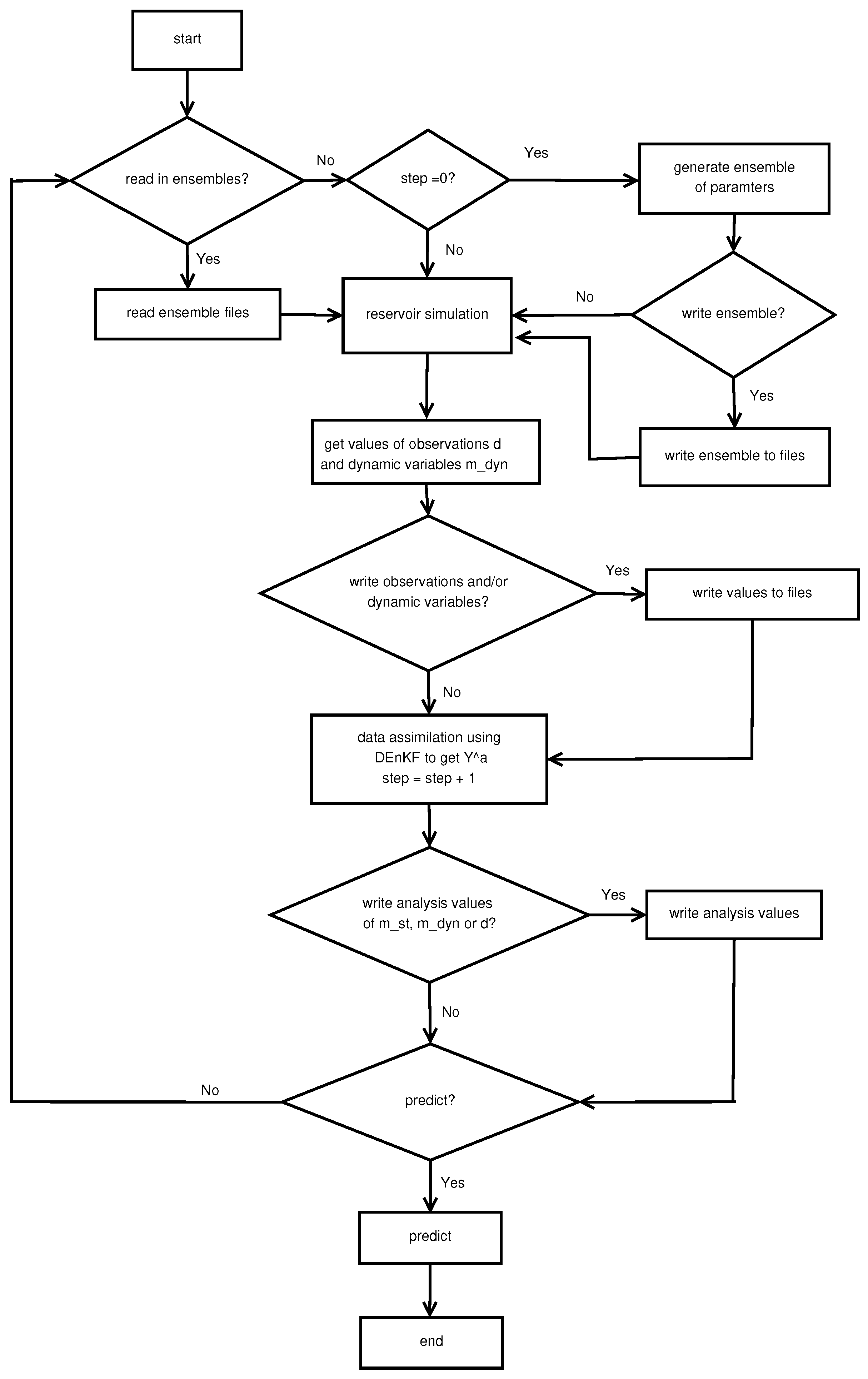
The flow chart of the implementation is given in Figure 1. In our implementation, for the result visualization purpose, two switches $writeens$ and $writepars$ can also be set by the user. When $writeens$ = TRUE, all the dynamic and static variables are written to the files but not necessarily read during running. When $writepars$ = TRUE, only static variables are written. The ensembles of the dynamic and static variables are always output to files at the last analysis step.

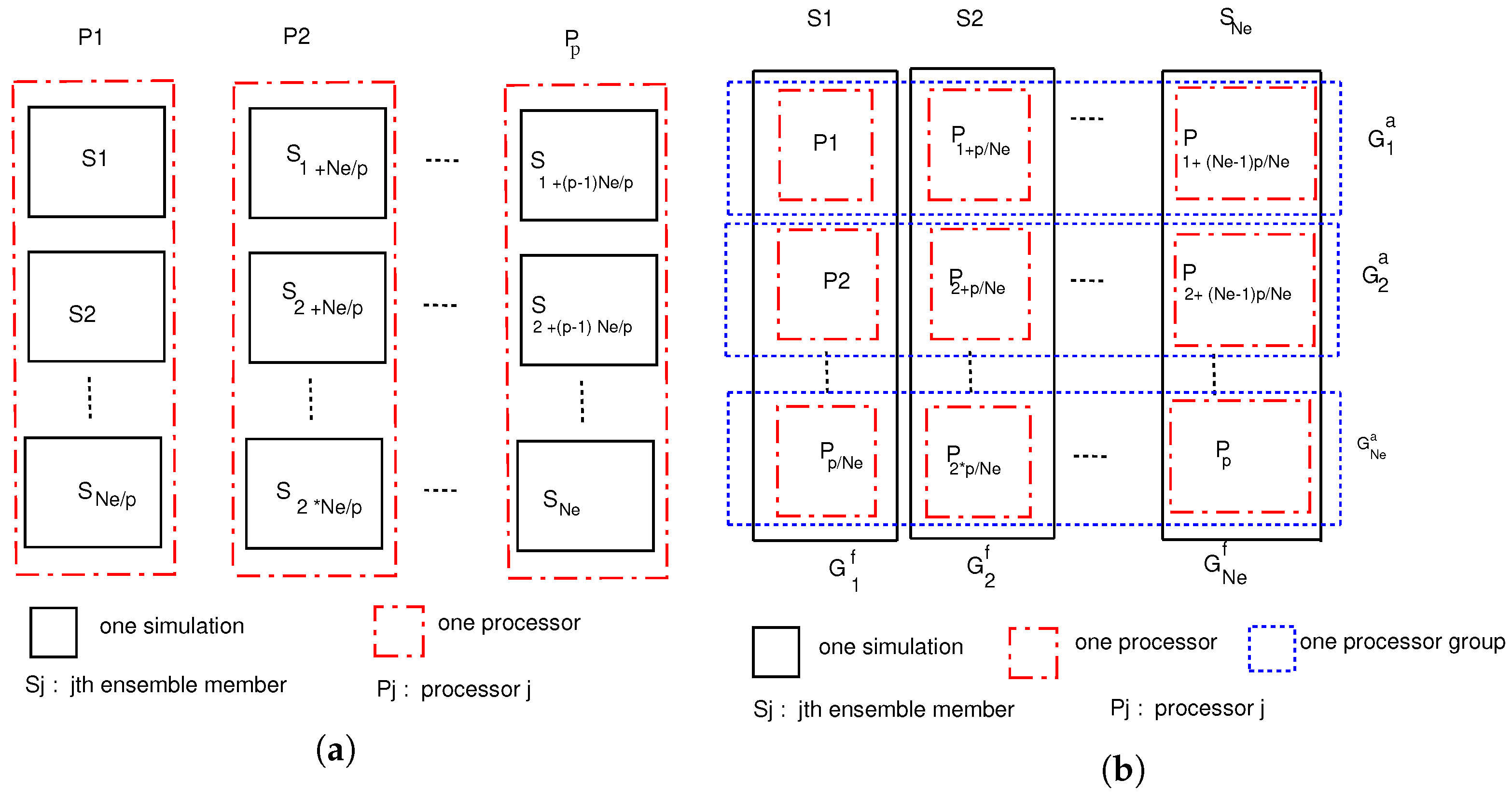
For the switch $readens$, if it is set to TRUE by the user, all the dynamic variables and the static variables are written to the files on a hard disk and the corresponding variable spaces allocated in the computer are freed after they are written at the each data assimilation step. After one cycle is done and before the next reservoir simulation starts, these data are read in from those files to restart the reservoir simulator. However, when the ensemble size is large, the performance of IO (Input and Output) is poor. Many small files written to the hard disk can not only waste space of the hard disk, but also are slow to access. The efficiency becomes even lower when the dynamic variable values are written to the files using MPI/IO. Nevertheless, MPI/IO must be used in a certain condition. For example, when the ensemble size is smaller than the processor size, for each ensemble, the reservoir simulation is done by several processors in parallel. Therefore, after the simulation, the vector of each dynamic variable is partially distributed in several processors. It is inevitable to write a dynamic vector to one file in the grid cell order using MPI/IO. To avoid reading and writing data to files, our simulator is slightly modified and the switch $readens$ can be set to FALSE by the user so that both the dynamic variables and the static variables are always in the memory during computing and their values are updated every step. One might worry about that these variables would occupy too much computer memory. In fact, the ensemble members are equally distributed in the processors from the beginning. The allocation of the ensemble members and the simulations in different processes are shown in Figure 2. In this figure, the solid box denotes one simulation, the dash dot box denotes one processor and the dot box denotes the processor group. If the ensemble size $N_e$ is larger than the processor number p, each processor only has $\frac{Ne}{p}$ ensemble numbers. If the ensemble size is smaller than the processor number, each simulation with one ensemble member is carried out by $\frac{p}{Ne}$ processors. The vector of each dynamic variable value is equally distributed to these $\frac{p}{Ne}$ processors. Therefore, when multiple computer nodes and CPU cores are used on a supercomputer, each core only spends limited memory to save the dynamic variable vectors. It is not costly to keep these variables all the time.

As an ensemble size is generally much smaller than the length of a state vector, the main computational cost of an analysis step is the matrix multiplication in Equation (7) which is computed in parallel after the matrix $X_5$ is computed sequentially by one processor. Supposing that the division of $N_e$ and p is an integer, there are two different cases:

• $N_e>p$. If the ensemble size $N_e$ is larger than the processor number p, each processor runs the simulation for $\frac{Ne}{p}$ times in every cycle independently and get the dynamic variable values corresponding to its ensemble members (see Figure 2a). Therefore, each processor obtains one or several complete columns of matrix $Y^f$. For processor $j(j=1,\cdots ,p)$, by multiplying these columns by $X_5$, it gets a matrix $Y^{a,j}$ with a size the same as that of matrix $Y^f$. Note that $Y^a={\sum }_{j=1}^p{Y}^{a,j}$ so the analysis results can be obtained by adding all the $Y^{a,j}$ from every processor using the function MPI_Allreduce. The matrix multiplication is illustrated by Figure 3.
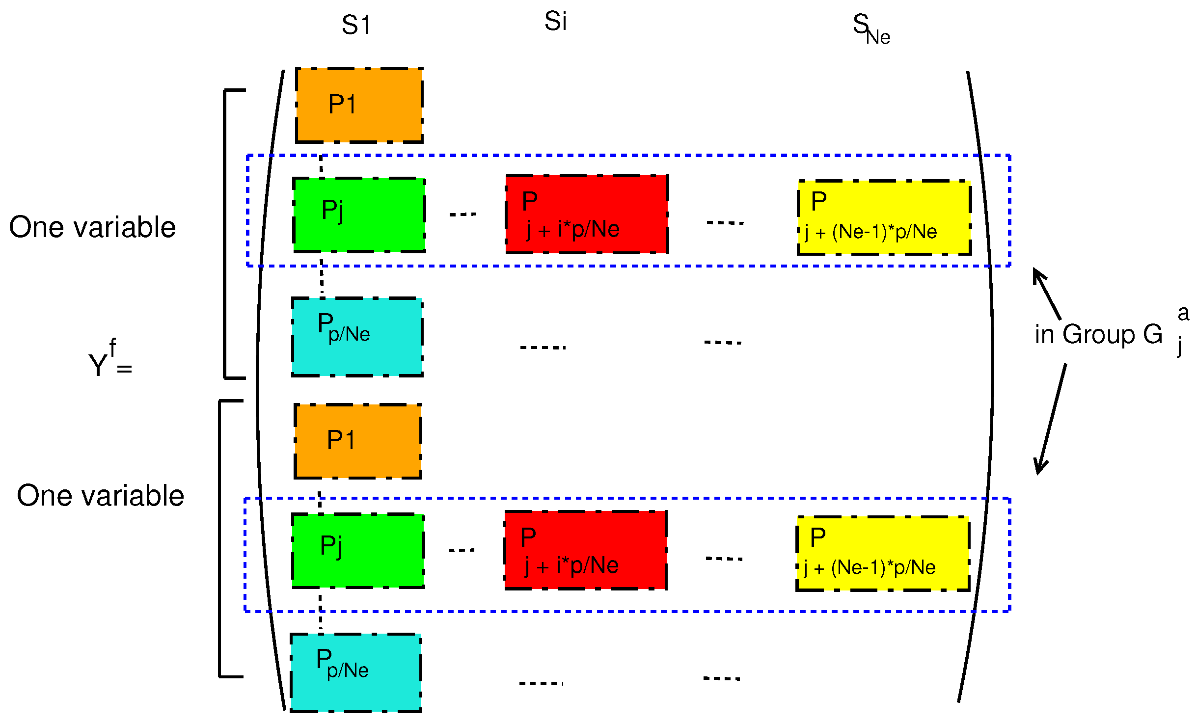
• $N_e<=p$. If the ensemble size $N_e$ is smaller than or equal to the processor number p, each simulation is done by the processor group $G_j^f$= {$P_{1+j\ast p/N_e}$, $P_{2+j\ast p/N_e}$, ⋯, $P_{p/N_e+j\ast p/N_e}$ }, $(j=0,\cdots ,N_e-1)$ (see Figure 2b) with $\frac{p}{N_e}$ processors included (note that they are at the same time in one simulation box). The computing tasks of the processors in this group are assigned by the simulator based on the domain decomposition. According to the load balancing principle, the vector entries of each dynamic variable are equally distributed and the variable values are not complete in each processor. For the processor group $G_j^a=\{P_j,P_{j+p/N_e},\cdots ,P_{j+(N_e-1)\ast p/N_e}\}$$(j=1,\cdots ,p/N_e)$ (see Figure 2b) by multiplying these vector entries of its own with $X_5$, the processors in Group $G_j^a$ get the matrices $Y^{a,j}$, $Y^{a,j+p/N_e}$,⋯$Y^{a,j+(N_e-1)\ast p/N_e},$ respectively. By gathering these values in its own group $G_j^a$, every processor in this group gets the value ${\sum }_{i=0}^{N_e-1}{Y}^{a,j+i\ast (p/N_e)}$ which includes the corresponding updated vector entries. The distribution of the matrix entries is displayed in Figure 4. The processor groups are created by the function lMPI_Comm_split.

When $N_e>p$ and the division of $N_e$ and p is not an integer, some of the processors get fewer ensemble members than the others and thus simulate a reservoir with less time. However, the algorithm is still the same. When $N_e<=p$ and the division of p and $N_e$ is not an integer, special treatment and more message passing are required when gathering the vectors since for some of the ensemble members the corresponding reservoir simulations are conducted by fewer processors than the others.

For a large-scale reservoir model that requires a large number of grid cells for discretization, the simulation with every ensemble member is time-consuming. In this case, the ensemble is not distributed to processors. Instead, the models with different ensemble members are simulated sequentially. Each model with one ensemble member is simulated by all the processors in parallel. Although the simulation run is very costly, it is obviously a trivial case of our discussion from the programming design aspect.

5. Numerical Experiments

In this section, the history matching of the SPE-9 benchmark model is presented. Estimations of relative permeability curves with known endpoints and unknown endpoints are plotted. With each estimation, the corresponding prediction results are obtained. Following that, the parallel efficiency of computations is reported.

5.1. SPE-9 Black Oil Model

SPE-9 is a three-phase black oil model with $24\times 25\times 15$ grid blocks. The grid sizes in the x- and y-direction are both 300 ft. The z-direction grid size is 20, 15, 26, 15, 16, 14, 8, 8, 18, 12, 19, 18, 20, 50, and 100 ft from top to bottom. It has heterogeneous absolute permeability. The porosity varies layer-by-layer in the z-direction and equals 0.087, 0.097, 0.111, 0.16, 0.13, 0.17, 0.17, 0.08, 0.14, 0.13, 0.12, 0.105, 0.12, 0.116 and 0.157 from top to bottom. The densities of water, oil and gas are 63.021, 44.986, and 0.0701955 lbm/ft3, respectively, with a reference pressure of 3600 psi. The bubble pressure is 3600 psi at the reference depth 9035 ft. The rock compressibility and water compressibility are both $1.0\times {10}^{-6}$ (1/psi). The total production days are 900 days.

There are 26 wells in the reservoir: one injector and 25 producers. The injector’s perforation is at layer 11 to layer 15 while each producer’s perforation is at layers 2, 3 and 4. The injector has a maximum standard water rate of 5000 bbl/day and a maximum bottom hole pressure of 4543.39 psi. The radius of each well is 0.5 ft. The schedule can be obtained from the keyword file in the document folder of the commercial software such as CMG IMEX.

The oil relative permeability in three phases can be obtained from the water and oil two-phase relative permeabilities and the gas and oil two-phase relative permeabilities [25]. To represent a relative permeability curve by a power-law function (e.g., based on an empirical Corey’s model [26]), a power-law model only requires to determine the endpoints and exponential factors. Power-law models of water and oil relative permeabilities can be written as

$$\begin{array}{ccc}\hfill k_{rw}\left(S_w\right)& =& a_w{\left(\frac{S_w-S_{wc}}{1-S_{wc}-S_{orw}}\right)}^{n_w}=a_w{S}_{wD}^{n_w}\hfill \end{array}$$

(8)

$$\begin{array}{ccc}\hfill k_{row}\left(S_w\right)& =& a_{ow}{\left(\frac{1-S_w-S_{orw}}{1-S_{wc}-S_{orw}}\right)}^{n_{ow}}\hfill \\ & & =a_{ow}{(1-S_{wD})}^{n_{ow}}.\hfill \end{array}$$

(9)

where

$$S_{wD}=\frac{S_w-S_{wc}}{1-S_{wc}-S_{orw}}.$$

Similarly, power-law representations of gas and oil relative permeabilities are

$$\begin{array}{ccc}\hfill k_{rg}\left(S_g\right)& =& a_g{\left(\frac{S_g-S_{gc}}{1-S_{gc}-S_{org}-S_{wc}}\right)}^{n_g}\hfill \\ & =& a_g{S}_{gD}^{n_g}\hfill \end{array}$$

(10)

$$\begin{array}{ccc}\hfill k_{rog}\left(S_g\right)& =& a_{og}{\left(\frac{1-S_g-S_{org}-S_{wc}}{1-S_{gc}-S_{org}-S_{wc}}\right)}^{n_{og}}\hfill \\ & =& a_{og}{(1-S_{gD})}^{n_{og}}.\hfill \end{array}$$

(11)

with

$$S_{gD}=\frac{S_g-S_{gc}}{1-S_{org}-S_{gc}-S_{wc}}.$$

Equations (8)–(11) will be used in our computing.

We consider the case where the oil relative permeability is defined by normalizing its effective permeability by using its value at the critical water saturation, i.e.,

$$k_{row}=\frac{k_{ow}\left(S_w\right)}{k_{ow}\left(S_{wc}\right)}$$

where $k_{ow}$ is the effective oil permeability. Then $k_{row}\left(S_{wc}\right)$ = 1 holds, which leads to $a_{ow}=1$. Similarly, for the gas and oil relative permeabilities, if the gas relative permeability is defined by normalizing its effective permeability by using its value at the irreducible gas saturation, i.e.,

$$k_{rog}=\frac{k_{og}\left(S_g\right)}{k_{og}\left(S_{gc}\right)}$$

where $k_{og}$ is the oil effective permeability, then $k_{rog}\left(S_{gc}\right)$ = 1 and thus $a_{og}=1$. Consequently, 10 parameters are left to define the relative permeability curves. Written as a parameter vector, they are

$$\begin{array}{ccc}\hfill {\mathbf{m}}_{st}& =& [a_w,n_w,n_{ow},S_{wc},S_{orw},\hfill \\ & & a_g,n_g,n_{og},S_{gc},S_{org}].\hfill \end{array}$$

(12)

Note that the endpoints are fixed by 6 parameters: $a_w$, $S_{wc},$$S_{orw},$$a_g$, $S_{gc}$ and $S_{org}$. If these parameters are known, only 4 parameters are left and the endpoints of the relative permeability curves are fixed. Thus, the parameter vector becomes

$${\mathbf{m}}_{st}=[n_o,n_{ow},n_g,n_{og}].$$

(13)

For an estimation with known endpoints, the observations are the cumulative water production rate (CWPR), cumulative oil production rate (COPR) and cumulative gas production rate (CGPR) of all the 25 production wells as well as the cumulative water injection rate (CWIR) of the injection well. For an estimation with unknown endpoints, the observations are the oil production rates, the gas production rates, the water production rates of the 25 producers, the water injection rate of the injector and the bottom-hole pressures of all the wells. All the rates are obtained from our simulator PRSI. All the data is perturbed by a Gaussian distribution error with 5% variance.

5.2. Estimation with Known Endpoints

As mentioned before, when the endpoints are known, only four unknowns are left as shown in Equation (13). In this work, totally 160 Gaussian realizations are generated for these parameters to assimilate the observations. The days on which the observations are assimilated are listed in

Table 1. The days on which data is assimilated.

step	1	2	3	4	5	6	7	8
day	12	32	50	67	87	102	122	141
step	9	10	11	12	13	14	15	16
day	162	182	200	217	237	257	277	297
step	17	18	19	20	21	22	23	24
day	312	332	352	367	387	407	422	442
step	25	26	27	28	29	30
day	462	480	497	517	537	552

. The first step of data assimilation is on the 12th day and the last one on the 552nd day. After that, each updated ensemble member with the permeability parameter values at the last step is used to simulate the model until the end day to predict the rates. The reference values, together with the means and the variances of the unknowns used to generate the ensemble, are listed in

Table 2. This table shows the reference values, the adjusted values and the relative errors at the last assimilation step, the initial ensemble means and variances of the four parameters in Equation (13).

Unknown	${\mathit{n}}_{\mathit{w}}$	${\mathit{n}}_{\mathit{ow}}$	${\mathit{n}}_{\mathit{g}}$	${\mathit{n}}_{\mathit{og}}$
reference value	5.5	4.0	2.0	3.0
adjusted value	5.86	4.03	2.02	3.23
relative error (%)	6.55	0.75	1.0	7.67
initial mean	4.0	3.0	1.5	2.0
initial variance	1.0	0.5	0.5	0.5

. The adjusted mean values after data assimilation and their relative errors different from the reference values are also listed in this table.

It turns out that the data assimilation is very effective. From Table 2, it is seen that the mean values of the initial ensemble are far from the reference values. However, after data assimilation, their values are quite close to the reference values with the relative errors ranging from 0.75% to 7.67%. The relative permeability curves are shown in Figure 5. It is seen that the initial curves are randomly scattered and the curves from the mean values are far from the reference ones. After assimilation, the adjusted curves almost overlap with the reference ones.

To show the parameter values more clearly, the variations of all the four parameters at different time are shown in Figure 6a–d, which depicts that the variation of each parameter becomes smaller by data assimilation. At the same time, the mean values become closer to the reference value. A relative root mean square error is calculated to show the convergence of the parameters. It is a normalized difference between the mean value of the updated parameter vector and its true value, i.e.,

$$R{E}_{st}=\sqrt{\frac{1}{N_{m_{st}}}{\displaystyle \sum _{i=1}^{N_{m_{st}}}}{\left(\frac{m_{st,i}^{\mathrm{mean}}-m_{st,i}^{\mathrm{true}}}{m_{st,i}^{\mathrm{true}}}\right)}^2}\times 100\%$$

(14)

where $m_{st,i}$ is the ith component of the vector ${\mathbf{m}}_{st}$ and $N_{m_{st}}$ is the length of the vector [9]. Figure 6e depicts the relative root mean square error of the relative permeability model vector. It shows that at the last assimilation step, the relative root mean square error drops to 5%.

From the 552nd day, the adjusted ensemble parameters from the last analysis step are used to predict the injection and production data. The cumulative oil production rate (COPR), the cumulative water production rate (CWPR) and the cumulative gas production rate (CGPR) of the group of all the 25 production wells as well as the cumulative water injection rate (CWIR) of the injection well are predicted and shown in Figure 7. In this figure, gray lines represent the rates from the initial ensemble. As the initial ensemble is randomly generated, the rates are quite different from each other. From day 12 to day 552 by the EnKF method, the observation data are assimilated 30 times, the permeability curves are adjusted and the new calculated and updated rates match the reference rates very well. After the last assimilation step, the adjusted permeability curves at day 552 are used to simulate the reservoir model to predict the rates. It is shown that the predicted rates and the reference rates almost overlap, which means that the adjusted permeability curves are accurate enough to be used to predict the future performance.

For the last analysis step, the relative errors of the pressure P, the water saturation $S_w$, the gas saturation $S_g$ and the well bottom hole pressure $P_{BH}$ are calculated by normalizing the difference of the ensemble mean and the variable’s true value. For each variable $\mathbf{v}$, the relative error is computed from the following form:

$$R{E}_{dyn}\left(\mathbf{v}\right)=\parallel {\mathbf{v}}^{\mathrm{mean}}-{\mathbf{v}}^{\mathrm{true}}{\parallel }_2/{\parallel {\mathbf{v}}^{\mathrm{true}}\parallel }_2$$

(15)

where ${\parallel ·\parallel }_2$ denotes the Euclidean norm of a discretized variable. The relative errors of these variables are listed in

Table 3. The relative errors of the dynamic variables $R{E}_{dyn}$ at the last assimilation step with known endpoints.

Dynamic Variables	P	${\mathit{S}}_{\mathit{w}}$	${\mathit{S}}_{\mathit{g}}$	${\mathit{P}}_{\mathit{BH}}$
relative errors (%)	0.63	0.28	2.5	0.93

. The table shows that the relative errors of the dynamic variables are no more than 2.5%. In particular, the pressure P, the water saturation $S_w$ and the well bottom hole pressure $P_{BH}$ are lower than 1.0%.

5.3. Estimation with Unknown Endpoints

For permeabilities with unknown endpoints, good estimations are not obtained by assimilating the observations of COPR, CWPR, CWIR and CGPR. It is probably because when the endpoints are unknown, the solution is not unique for this inverse problem. Therefore, we assimilate more detailed data including the oil production rates (WOPR), the water production rates (WWPR), the gas production rates (WGPR) of the 25 producers, the water injection of the injector (WWIR) and the bottom-hole pressures (WBHP) of all the wells. It is interesting to see that with more data assimilated and an ensemble with 640 samples, all the parameters are well estimated.

Table 4. This table shows the reference values, the adjusted values and the relative errors $R{E}_{st}$ at the last assimilation step, the initial ensemble means and variances of the ten parameters in Equation (12).

Unknown	${\mathit{a}}_{\mathit{w}}$	${\mathit{n}}_{\mathit{w}}$	${\mathit{n}}_{\mathit{ow}}$	${\mathit{S}}_{\mathit{wc}}$	${\mathit{S}}_{\mathit{orw}}$	${\mathit{a}}_{\mathit{g}}$	${\mathit{n}}_{\mathit{g}}$	${\mathit{n}}_{\mathit{og}}$	${\mathit{S}}_{\mathit{gc}}$	${\mathit{S}}_{\mathit{org}}$
reference value	0.5	5.5	4.0	0.156572	0.123639	0.8	2	3	0.02	0.1
adjusted value	0.5619	5.3012	4.4599	0.1520	0.1248	0.8657	2.0327	3.0537	0.0192	0.0882
relative error (%)	12.38	3.62	11.50	2.92	0.93	8.22	1.63	1.79	3.88	11.81
initial mean	0.6	4	2.0	0.3	0.05	0.6	1.5	2.0	0.05	0.05
initial variance	0.3	1.0	0.5	0.03	0.03	0.3	0.5	0.5	0.02	0.03

shows the reference values, the adjusted values, the relative errors, the initial ensemble means and variances. From this table, we can see that most of the relative errors are no more than 10% except $a_w$, $n_{ow}$ and $S_{org}$ which are ~12%. Figure 8 shows the relative permeability curves of oil-water and oil-gas. We can see that although the initial curves are quite random, the updated curves are close to the reference curves.

Similar to the previous example, the variations of all the ten parameters at different time are also plotted (see Figure 9a–j). This figure depicts that the variations of parameters become smaller by data assimilation. At the same time, the mean values become closer to the reference values. Figure 9k shows that from the beginning to the last data assimilation step, the relative mean-square-root error of all the ten parameters drops from 65.5% to 8.4%.

For the prediction step, the injection/production rates obtained from the adjusted parameters match the observation very well. The results of WOPR, WWPR, WGPR and WBHP of some selected wells including Producer1, Producer 4, Producer 8 and Producer 20 are depicted in Figure 10. For each well, the relative error of one prediction variable is calculated from the mean-square-root of the observation variable on $N_D$ days included in the set D = {565, 600, 601, 604, 610, 625, 660, 661, 664, 670, 685, 720, 721, 724, 730, 745, 783, 873, 900} using the following formula:

$$R{E}_{\mathrm{predict}}=\sqrt{\frac{1}{N_D}\sum _{i\in D}\frac{|d_i^{\mathrm{mean}}-d_i^{\mathrm{true}}{|}^2}{|d_i^{\mathrm{true}}{|}^2}}$$

where $d_i^{\mathrm{mean}}$ and $d_i^{\mathrm{true}}$ denote the mean and true values of one observation variable d on the ith day, respectively. The values of the relative errors are shown in the bar graphs in Figure 11. This figure shows that with the estimated parameters, the relative errors of the predicted rates and the well bottom-hole pressure are no more than 3.5%. The relative errors of the dynamic variables at the last analysis step calculated by Equation (15) are listed in

Table 5. The relative errors of the dynamic variables $R{E}_{dyn}$ at the last assimilation step with unknown endpoints.

Dynamic Variables	P	${\mathit{S}}_{\mathit{w}}$	${\mathit{S}}_{\mathit{g}}$	${\mathit{P}}_{\mathit{BH}}$
relative error (%)	0.61	4.28	1.98	0.94

. This table shows that the relative errors of the dynamic variables are no more than 4.28%.

5.4. Parallel Performance and Discussion

The numerical experiments are carried out on the Niagara Scinet cluster of 1548 Lenovo SD 530 servers each with 40 Intel ‘Skylake’ cores at 2.4 GHz. To test the MPI parallel performance of our computing, the examples of both known endpoints and unknown endpoints in the previous section are computed with 40, 80, 160, 320 and 640 cores. In these computations, the switch $readens$ is set to FALSE. Therefore, only the ensembles at the last analysis step are output to files. To compare more precisely, the initial ensemble is generated in advance and read from the disk at the beginning of each run. Both experiments are computed with one processor per CPU core. The 40-core case is used as the base case. Computational time is given for both of the examples. The parallel efficiency and the speedup are presented. Generally, the parallel efficiency is defined as

$$E_p=\frac{T_1}{T_{p}p}$$

where $T_1$ and $T_p$ denote the run time of a task using one processor and p processors, respectively. $T_1$ is the base case time. If the execution time of $p_0$ processors is used as a base case, the parallel efficiency can be calculated by

$$E_p=\frac{T_{p_0}{p}_0}{T_{p}p}.$$

The speedup is defined as

$$S_p=\frac{T_1}{T_p}.$$

Similarly, if the execution time of $p_0$ processors is used as a base case, the speedup can be calculated by

$$S_p=\frac{T_{p_0}}{T_p}.$$

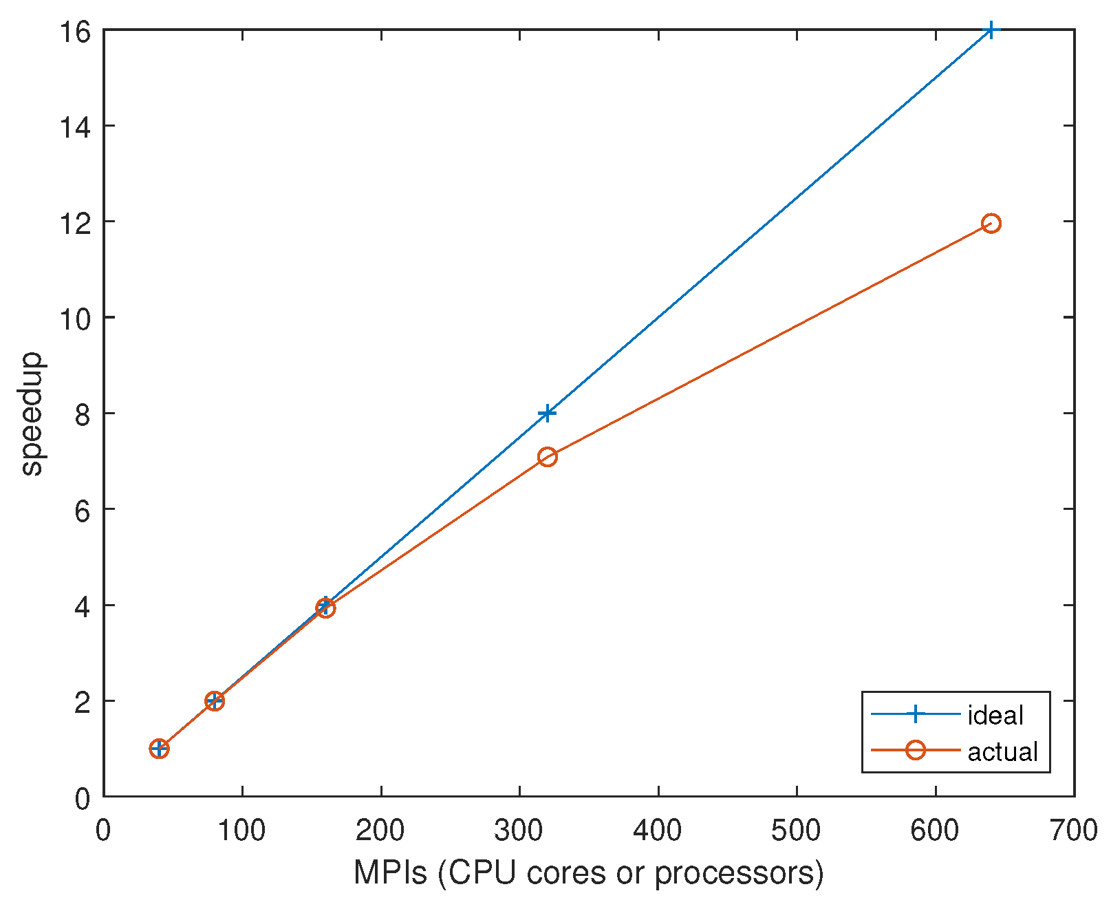
For the known endpoint experiment with 160 ensemble members, the computational time and parallel efficiency are listed in

Table 6. The computational time and parallel efficiencies for the known endpoint example (time unit: second).

CPU Cores	40	80	160	320	640
forecast	464	228	114	60	36
analysis	11	9	7	5	4
predict	98	50	24	15	7
other	1	1	1	1	1
run time	574	288	146	81	48
$E_P$(%)	-	99.65	98.29	88.58	74.74

. In this table, the ‘forecast’ denotes the total forecast time including the synchronization time. The ‘analysis’ is the total time spent on the analysis step. The ‘predict’ denotes the prediction time after the last step of analysis. The ‘other’ time mainly includes the run time of input/output. The last row ‘run time’ is the total execution time. From this table, it can be seen that most time is spent on the forecast steps and the prediction steps. With the CPU cores increasing, the run time decreases rapidly. When 40, 80 and 160 CPU cores are used, the time for the forecast steps is reduced by half when the CPU core number is doubled. This also happens at the prediction steps. Therefore, we can see that the parallel efficiencies of the forecast and the prediction steps are over 100%. When 320 and 640 CPU cores are used, the ensemble size is 160 which is smaller than the processor numbers. Each simulation is conducted by multiple CPU cores which needs message passing. Therefore, the parallel efficiencies of the forecast and prediction steps are lower than 100%. The last row shows that the parallel efficiency of the whole execution is over 74% compared to the ideal efficiency 100%. Note that the parallel efficiency of the analysis step is not as good as the forecast and prediction as the time for the multiple message passing becomes dominant in the analysis step when more processors are used. The speedup is shown in Figure 12. It can be seen from this figure that when 40, 80 and 160 CPUs are used, the speedup is almost linear. This benefits from the good parallel efficiencies of the forecast steps and the prediction steps. When 320 and 640 CPU cores are used, it drops down and becomes sub-linear.

For the unknown endpoint experiment with 640 ensemble members, the time and the parallel efficiencies are shown in

Table 7. The computational time and parallel efficiencies for the unknown endpoint example (time unit: second).

CPU Cores	40	80	160	320	640
forecast	2060	1034	561	275	136
analysis	103	62	53	49	41
predict	431	215	110	55	28
other	2	2	2	3	4
run time	2596	1313	726	382	209
$E_P$(%)	-	98.86	89.39	84.95	77.26

. From this table, it can be seen that all steps take more time than those with the known endpoint example since the ensemble size is much larger. Similar to the previous example, good parallel efficiencies of the forecast and the prediction steps are obtained, as here the ensemble size is always less or equal to the processor number, which means each simulation is conducted by one processor independently with no message passing required. The run time reduces significantly when more CPU cores are used. The parallel efficiency is over 77%. The time for the analysis also reduces with more CPU cores are used. However, it can be seen that the parallel efficiencies for this step is much lower than the ideal one. One reason is that the observation reading time does not decrease with the number of CPU cores increasing. Another reason is that several times of message passing are required to obtain the updated ensemble in the analysis steps.

To show the time allocation of the analysis step in detail, the time spent on every part of the last analysis step is listed in

Table 8. The time allocation at the last analysis step for the unknown endpoint example (time unit: second).

CPU Cores	40	80	160	320	640
read obs	0.24	0.25	0.20	0.24	0.27
compute $X_5$	0.05	0.08	0.07	0.09	0.09
$A^f\ast X_5$	2.27	1.16	0.73	0.45	0.30
MPI_Allreduce	0.40	0.35	0.39	0.62	0.58
output	2.98	1.41	1.45	0.67	0.65
total	5.54	3.25	2.84	2.07	1.89

. In this table, ‘read obs’ means the time used for reading observations from the files. The term ‘compute $X_5$’ means the time for computing matrix $X_5$. The term ‘$A^f\ast X_5$’ denotes the time used for the multiplication of the local forecast ensemble and matrix $X_5$. The term ‘MPI_Allreduce’ denotes the message passing time used in the analysis step. The term ‘output’ denotes the time used for the ensemble output. The ‘total’ denotes the total time of this analysis step. From the second row ‘read obs’ and the third row ‘compute $X_5$’, it can be seen that the time for computing matrix $X_5$ is very short compared to the others. From the fourth row ‘$A^f\ast X_5$’, it can be seen that the time used for the matrix multiplication reduces significantly when more CPU cores are used. Compared to the time used for message passing shown in the fifth row ‘MPI_Allreduce’, it becomes less dominant with the CPU cores increasing. The time for reading observations and the message passing does not reduce when more CPU cores are used, which leads to the low parallel efficiencies for the analysis steps. The ‘output’ row shows that when more CPU cores are used, the time used for outputting the ensemble is also reduced somehow. The speedup curve of the whole execution is plotted in Figure 13 which shows better performance than the known endpoint example.

6. Conclusions

A parallel technique is used to implement the DEnKF for reservoir history matching. The algorithm and implementation are introduced in detail. Two numerical experiments of estimating relative permeabilities are computed using a massively parallel computer. Reservoir history matching using DEnKF can be efficiently implemented using the MPI parallel technique. The parallel efficiency is over 74% for a small ensemble with 160 members and 77% for a large ensemble with 640 members using up to 640 CPU cores.

The numerical experiments demonstrate that the DEnKF can be used to estimate the relative permeability curves given by a power-law model in reservoir history matching. For the relative permeability curves with known endpoints, all the parameters in a power-law model can be estimated well. For the unknown endpoint model, good estimations can be obtained with more observations and a larger ensemble size compared to the known endpoint model.

References

- Evensen, G. The Ensemble Kalman Filter: Theoretical formulation and practical implementation. Ocean Dyn. 2003, 53, 343–367. [Google Scholar] [CrossRef]
- Sakov, P.; Oke, P.R. A deterministic formulation of the ensemble Kalman filter: An alternative to ensemble square root filters. Tellus 2008, 60A, 361–371. [Google Scholar] [CrossRef] [Green Version]
- Nævdal, G.; Mannseth, T.; Vefring, E.H. Near-well reservoir monitoring through ensemble Kalman filter. In Proceedings of the SPE/DOE Improved Oil Recovery Symposium, Freiberg, Germany, 3–6 September 2002. [Google Scholar]
- Nævdal, G.; Johnsen, L.M.; Aanonsen, S.I.; Vefring, E.H. Reservoir Monitoring and continuous model updating using ensemble Kalman filter. SPE J. 2005, 10, 66–74. [Google Scholar] [CrossRef]
- Aanonsen, S.I.; Nævdal, G.; Oliver, D.S.; Reynolds, A. The ensemble kalman filter in reservoir engineering—A review. SPE J. 2009, 14, 393–412. [Google Scholar] [CrossRef]
- Gu, Y.; Oliver, D.S. History matching of the PUNQ-S3 reservoir model using the ensemble Kalman filter. SPE J. 2005, 10, 217–224. [Google Scholar] [CrossRef]
- Lorentzen, R.J.; Nævdal, G.; Vallès, B.; Berg, A.M.; Grimstad, A.A. Analysis of the ensemble Kalman filter for estimation of permeability and porosity in reservoir models. In Proceedings of the SPE Annual Technical Conference and Exhibition, Dallas, TX, USA, 9–12 October 2005. [Google Scholar] [CrossRef]
- Chen, S.; Li, G.; Peres, A.; Reynolds, A.C. A well test for In-Situ determination of relative permeability curves. SPE J. 2008, 11, 95–107. [Google Scholar] [CrossRef]
- Li, H.; Chen, S.N.; Yang, D.; Tontiwachwuthikul, P. Estimation of relative permeability by assisted history matching using the ensemble Kalman filter method. Pet. Soc. Can. 2012, 51, 205–213. [Google Scholar] [CrossRef]
- Zhang, Y.; Song, C.; Yang, D. A damped iterative EnKF method to estimate relative permeability and capillary pressure for tight formations from displacement experiments. Fuel 2016, 167, 306–315. [Google Scholar] [CrossRef]
- Zhang, Y.; Yang, D. Simultaneous estimation of relative permeability and capillary pressure for tight formation using ensemble-based history matching method. Comput. Fluids 2013, 71, 446–460. [Google Scholar] [CrossRef]
- Keppenne, C.L.; Rienecker, M.M. Initial testing of a massively parallel ensemble Kalman filter with the Poseidon isopycnal ocean general circulation model. Mon. Weather Rev. 2002, 130, 2951–2965. [Google Scholar] [CrossRef] [Green Version]
- Houtekamer, P.L.; Mitchell, H.L. A sequential ensemble Kalman filter for atmospheric data assimilation. Mon. Weather Rev. 2001, 129, 123–137. [Google Scholar] [CrossRef]
- Liang, B.; Sepehrnoori, K.; Delshad, M. An automatic history matching module with distributed and parallel computing. Pet. Sci. Technol. 2009, 27, 1092–1108. [Google Scholar] [CrossRef]
- Tavakoli, R.; Pencheva, G.; Wheeler, M.F.; Ganis, B. A parallel ensemble-based framework for reservoir history matching and uncertainty characterization. Comput. Geosci. 2013, 17, 83–97. [Google Scholar] [CrossRef]
- Tavakoli, R.; Pencheva, G.; Wheeler, M.F. Multi-level parallelization of ensemble Kalman filter for reservoir history matching. In Proceedings of the SPE Reservoir Simulation Symposium, The Woodlands, TX, USA, 21–23 February 2011. [Google Scholar] [CrossRef]
- Sakov, P.; Oke, P.R. Implications of the form of the ensemble transformation in the ensemble square root filters. Mon. Weather Rev. 2008, 136, 1042–1053. [Google Scholar] [CrossRef] [Green Version]
- Evensen, G. Sampling strategies and square root analysis schemes for the EnKF. Ocean Dyn. 2004, 54, 539–560. [Google Scholar] [CrossRef]
- Chen, Z. Reservoir Simulation: Mathematical Techniques in Oil Recovery. CBMS-NSF Regional Conference Series in Applied Mathematics; SIAM: Philadelphia, PA, USA, 2007; Volume 77. [Google Scholar]
- Chen, Z.; Huan, G.; Ma, Y. Computational Methods for Multiphase Flows in Porous Media. Computational Science and Engineering Series; SIAM: Philadelphia, PA, USA, 2006; Volume 2. [Google Scholar]
- Chen, Z.; Espedal, M.; Ewing, R.E. Finite element analysis of multiphase flow in groundwater hydrology. Appl. Math. 1994, 40, 203–226. [Google Scholar] [CrossRef]
- Wang, K.; Liu, H.; Chen, Z. A scalable parallel black oil simulator on distributed memory parallel computer. J. Comput. Phys. 2015, 301, 19–34. [Google Scholar] [CrossRef]
- Burgers, G.; Leeuwen, P.J.V.; Evensen, G. Analysis scheme in the ensemble Kalman filter. Mon. Weather Rev. 1998, 126, 1719–1724. [Google Scholar] [CrossRef]
- Sakov, P. EnKF-C User Guide, Version 1.64.2. 2014. Available online: https://github.com/sakov/enkf-c (accessed on 1 January 2020).
- Stone, H.L. Probability Model for estimating three-phase relative permeability. J. Pet. Technol. 1970, 22, 214–218. [Google Scholar] [CrossRef]
- Reynolds, A.C.; Li, R.; Oliver, D.S. Simultaneous estimation of absolute and relative permeability by automatic history matching of three-phase flow production data. J. Can. Pet. Technol. 2004, 43. [Google Scholar] [CrossRef]
Figure 1.
The flowchart of the algorithm.
Figure 2.
The allocation of the ensemble members and the simulations in different processors: (a) and (b) .
Figure 3.
The matrix multiplication of and in case . (i = 1, ⋯, p) denotes the ith processor.
Figure 4.
The entries of the matrix on different processors in case (i = 1, ⋯, ) denotes the ith ensemble member. (i = 1, ⋯, p) denotes the ith processor.
Figure 5.
Initial ensembles, initial ensemble means, adjusted values and reference values with known endpoints: (a) and ; (b) and .
Figure 6.
The reference values, the adjusted parameters and the relative root mean square errors the at different time with known endpoints. The red line denotes the true reference (true) value of a parameter. The black dot denotes the mean of an ensemble. The blue bar denotes the maximum and minimum deviations from the mean. (a) ; (b) ; (c) ; (d) ; (e) the relative root mean square error.
Figure 7.
The production rates with known endpoints: (a) cumulative oil production rate; (b) cumulative water production rate (The upper curve is the cumulative water injection rate. The lower curve is the cumulative water production rate); (c) cumulative gas production rate.
Figure 8.
Initial ensembles, initial ensemble means, adjusted values and reference values with unknown endpoints: (a) and ; (b) and .
Figure 9.
The reference values, the adjusted parameters and the relative root mean square errors the at different time with unknown endpoints. The red line denotes the true reference (true) value of a parameter. The black dot denotes the mean of an ensemble. The blue bar denotes the maximum and minimum deviations from the mean.
Figure 10.
The oil production rates, the water production rates, the gas production rates and the bottom-hole pressure of the selected production wells with unknown endpoints.
Figure 11.
The relative errors of the prediction of all the wells.
Figure 12.
The speedup for the known endpoint example with 160 ensemble members.
Figure 13.
The speedup for the unknown endpoint example with 640 ensemble members.