Condition Monitoring of Drive Trains by Data Fusion of Acoustic Emission and Vibration Sensors ^†

Abstract

Early damage detection and classification by condition monitoring systems is crucial to enable predictive maintenance of manufacturing systems and industrial facilities. Data analysis can be improved by applying machine learning algorithms and fusion of data from heterogenous sensors. This paper presents an approach for a step-wise integration of classifications gained from vibration and acoustic emission sensors in order to combine the information from signals acquired in the low and high frequency ranges. A test rig comprising a drive train and bearings with small artificial damages is used for acquisition of experimental data. The results indicate that an improvement of damage classification can be obtained using the proposed algorithm of combining classifiers for vibrations and acoustic emissions.

1. Introduction

Increasing demand for efficient, reliable and available industrial production systems has led to the development of systems for continuous condition monitoring (CM). By the analysis of sensor signals, failures and wear can be detected in an early stage, enabling cost-effective predictive maintenance and prohibiting severe damages [1,2,3]. A widely implemented application is CM of bearings. These are critical parts of many industrial drives. Established fields of application include wind energy [4] or process industry [5].

A common monitoring approach includes vibration measurements, usually conducted with accelerometers [6]. Damage detection is traditionally carried out by the extraction of features from the time domain signals or the respective frequency domain representation. An overview of commonly used features such as RMS, Variance or Kurtosis, especially with application to low speed bearings, is given in [7]. Since bearings exist in a wide range of geometries and are driven at different speeds and loads, CM systems have to be adapted individually for a sufficient damage detection capability [8]. Still, the performance of vibration-based CM systems suffers when dynamic acceleration levels become low due to slow rotation speeds, when disturbance levels are high due to coupling with noisy gearboxes or other drive train components, and in case of varying speeds.

In many practical cases of vibration analysis for CM, the relevant signals are deteriorated by background noise or interference. The Wiener filter technique is suitable for these tasks, for slowly varying disturbances, and adaptive digital filters can also be applied [9]. Originating from the removal of interference from signals in the medical diagnostic sector, the removal of noise and interference from bearing vibration signals has been implemented [10]. One option is the utilization of a reference correlated to the interfering signal, a technique also applied in active noise control systems [11]. Another option is the so-called adaptive line enhancer, which does not need a dedicated reference. This method has already been tested in real industrial environments [12].

Measurement of vibration at higher frequencies between 35 and 40 kHz was tested decades ago, and a higher sensitivity to bearing wear could be proven [13]. Additionally, CM based on ultrasonic structure-borne noise or acoustic emissions has been evaluated [14,15]. The method is based on the detection of impulsive events (bursts) sent out from the rolling contact of damaged bearing elements. One of the first applications were the large and slowly rotating main bearings in off-shore cranes [16]. Several works investigated the performance of vibration and ultrasonic CM in comparison to each other, demonstrating the high sensitivity of Acoustic Emission (AE), e.g., for monitoring of gearboxes [17] and bearings [18]. While being very sensitive, disadvantages of the method include limited range of the impulsive waves in the structure and being insensitive to global mechanical faults such as misalignment of drive shafts, imbalances or loose parts [19]. Another challenge in comparison to vibration signals is the high data rate resulting from the needed sampling frequency of AE signals [20].

For both methods, the vibration approach and ultrasonic approach, a number of signal analysis algorithms have been developed, either in the time or frequency domain. More recent approaches use the corresponding sensor data as an input to powerful machine learning (ML) algorithms [21,22,23,24]. ML has been successfully applied in a previous work to this paper for the detection of mechanical faults such as imbalances [1]. Several works investigated how data from multiple vibration sensors can be jointly processed to obtain diagnostic information about a rotating machine [25,26,27].

AE signatures can estimate the remaining useful life of a slowly rotating bearing [28]. A fatigue test introduced flat spots to the bearing rings. However, the AE signatures were not analyzed in depth to distinguish between different damage types. Hase investigated the influence of damages on the AE signatures in a fatigue test. Different damages could be distinguished both in the time and frequency domains. However, an attempt for automation of classification by machine learning was not reported [29]. An application of machine learning to the classification of AE signatures of a sliding bearing in a fatigue test was presented in [30]. A deep neural network classified different damages, but a limited accuracy was reached. Saufi et al. applied a classification to several features of vibration and AE signals generated from rotating bearings. Different artificial defects could be distinguished; however, no attempt for data fusion was described [31]. Support Vector Machines (SVMs) were applied to classify AE signals from artificially damaged bearings. The input features of the SVM were skewness and kurtosis calculated from the measured signals. Classified damages included cracks in the outer ring of the bearing and debris [32].

Additionally, fusion of heterogeneous sensors has been investigated. The authors of [33] give an overview and a taxonomy of the approaches: with respect to the analysis layer that implements the fusion method, data fusion, feature fusion, and decision fusion can be distinguished. For an example of decision fusion, in [3], an approach based on fusion of AE and vibration signals is presented. Classifiers for both signals are trained and afterwards merged by a random forest network to detect gearbox faults. Further approaches to detect gearbox faults use information from multiple motor current sensors [34] or from vibration sensors and rotary encoders [35] for a neural network-based classification. In [36], features from various heterogenic sensor time series are extracted, decorrelated using principle component analysis and afterwards classified using a naïve Bayes classifier to detect motor faults. The fusion of two-dimensional image data from an infrared camera with one-dimensional vibration signals using convolutional neural networks and t-distributed stochastic neighbor embedding is shown in [37].

CM with integrated sensors or by acquisition of operation parameters supports the continuous analysis of the system’s state. A CM system, thus, can improve resilience, if a feedback loop automatically switches operation modes according to the detected state of the system components. On the other hand side, the CM itself is a system component and has to provide a resilient behavior. Especially for critical systems, the CM function should still provide a defined minimum of functionality in case some of its components fail. This is also supported by a heterogeneous sensor architecture: a common mode failure, i.e., several sensors failing due to the same cause being prevented [38]. If one sensor fails, the remaining sensors can still provide data for CM. In the best case, both sensors are operating, and their data can be fused for an improved analysis.

The aim of this work is to provide a novel approach for data fusion of vibration and AE signals with a realistic test bench for bearing damage detection. In particular, several damage types should be classified, even if the setup is dismantled and reassembled between the measurements of the data used for model training and validation. The system concept comprises an interference canceling at the input stage, and also a parallel implementation of a feature fusion approach and isolated classifiers for both sensor systems. This enables an analysis of the benefit with respect to the system complexity. In addition, the resulting CM system is resilient against a single sensor failure due to the remaining isolated classifier which is based only on the remaining sensor. The source code used for this work is available at Github [39].

2. Methods

In this section, the used drive train setup will be explained first (Section 2.1). Specifications of the conducted measurements will be given in the same section. The conducted data preprocessing steps will be described in Section 2.2. The used approach, the data from the AE and vibration sensors as well as the rotation speed information are used to calculate a combined classification, as shown in Section 2.3. Its actual implementation follows in Section 2.4.

2.1. Experimental Setup and Measurement

The proposed approach is demonstrated with a drive train setup, at which multiple bearing failures can be simulated (see Figure 1). It follows the basic concept documented in [1] and is extended by an instrumentation with AE sensors. The setup comprises a cage rotor induction motor (WEG V3.5111) connected to a bearing shaft by a flexible coupling, driven by an electronic motor inverter that allows the output rotation speed to be set by the operator. The velocity of the shaft was determined using a consumer-grade digital laser tachometer (Akozon DT2234C+) and was controlled via a potentiometer connected to the inverter unit. The inverter uses the feedback of the motor to ensure a constant rotational speed after setting it with the aforementioned potentiometer.

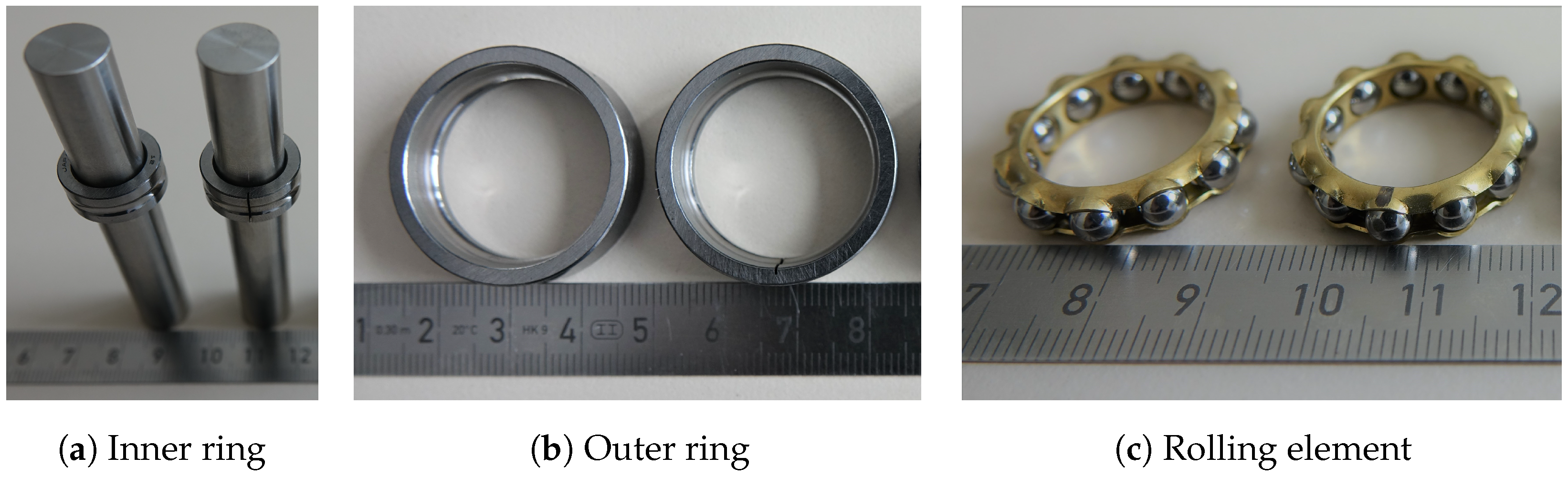
The simulated bearing failures include damaged outer rings, damaged inner rings and damaged rolling elements. All the aforementioned failures are tested in two severities; this means that one small slot and one larger slot are inserted into the inner ring and the outer ring. Instead of a slot, the defect at the rolling element is a flat spot. The damaged parts as well as their counterparts without damage are depicted in Figure 2. The bearings are precision magneto ball bearings of type E12 (DIN 615) (12 × 32 × 7 mm), which are essentially deep groove ball bearings with an outer ring with only one shoulder, providing a separable outer ring from the cage and inner ring. The cage allows removal from the inner ring and individual bearing balls within the cage can be swapped. Thus, with this type of bearing it is possible to selectively mount individual defects or defect combinations. Damages of different sizes are introduced to the inner rings, the outer rings and the rolling elements by wire electrical discharge machining (EDM). The defect sizes were chosen in relation to the diameter of the rolling elements of 4.7 mm. For the cases of inner and outer rings, slots with widths of 8% and 40% in relation to the ball diameter were inserted (corresponding to 376 and 1880 $\mathsf{\mu }$m each). A flattening was introduced to the rolling elements with depths of 2% and 8% of the rolling element diameter (corresponding to 94 and 376 $\mathsf{\mu }$m each). The precision of the wire EDM amounts to ±10 $\mathsf{\mu }$m. The relative dimensions of the bearing damages are are thus in a similar range to those reported in [31], where damages in the range between 9.6% and 28.8% of the rolling element diameter were used.

For vibration measurements, the setup is instrumented with ICP accelerometers (PCB 607A11, 100 mV/g, 0.5 Hz–10,000 Hz) at the bearing holder frame of the motor and the bearing holder frame of the shaft. Both vibration sensors are digitized by a DT 9837A USB-DAQ from Measurement Computing GmbH. This 4-channel signal analyzer is equipped with a 24-bit ADC, which supports sample rates of up to 100 kSPS and is well suited for the vibration measurements. AE signals were acquired by a piezo transducer (Vallen VS30V, 20 kHz–80 kHz) connected to an AEP5 preamplifier for signal conditioning. These signals were digitized with an USB oscilloscope (PicoScope 2204A: 2-channel, 8-bit ADC, sample rate up to 100 MSPS, analog bandwidth of 10 MHz). Both sensors were connected to a single board computer (Raspberry Pi 3B+) running custom software to acquire both data streams simultaneously. Data were stored in two separate files. However, all data could be synchronized afterwards by frequently incorporating precise time-stamps into the files. This synchronization was carried out using the system clock of the single board computer and thus did not include USB-related delays. Therefore, the overall synchronization performance was estimated to be ±10 ms.

In order to separate the effect of mounting a damaged bearing from variability of the setup when demounting and mounting due to uncertainties in torque of screws, orientation of damage at the bearing, etc., measurements were repeated several times after demounting and mounting the bearing. For the case of the outer ring defect, the orientation of the defect was varied within the angles −45°, 0° and 45° with respect to the vertical, which resulted in a higher number of measurements for this defect type. In total, data from 29 measurements were collected and used to train the neural network-based classifiers, as explained in the following sections. Measurements were conducted at five different speeds (600/1000/1400/1800/2200 rpm) and with different damaged bearings mounted.

Table 1. Parameters of used datasets.

Defect Type	No Defect	Inner Ring Defect		Outer Ring Defect		Rolling Element Defect
Defect Size	-	376 $\mathsf{\mu }$m	1880 $\mathsf{\mu }$m	376 $\mathsf{\mu }$m	1880 $\mathsf{\mu }$m	94 $\mathsf{\mu }$m	376 $\mathsf{\mu }$m
Number of measurements development dataset	3	3	3	4	3	3	3
Number of measurements validation dataset	1	1	1	1	1	1	1

lists the number of measurements obtained together with their respective specifications. There is one measurement for each specification, which is not used for model training but holds out for the validation of the trained classifiers. These measurements represent the validation dataset, while the other measurements are referred to as the development dataset.

2.2. Data Preprocessing

For the classification, vibration signals from the sensor mounted close to the bearing were used. The acquired vibration data contain a significant DC offset, since the accelerometers were powered over the signal line. A Bessel high pass filter of order 4 and a cut-off frequency were applied to the vibration signal. With a roll-off of 80 dB per decade, it allowed for a sharp separation of the information contained in the vibration from the offset. By applying the filter to time series twice, forwards and backwards, the effective order of the filtering operation doubled, while the phase lag was compensated. Details on the design of digital filters can be found in [40]. The algorithms are well established and part of standard libraries such as Scipy [41], which was used here.

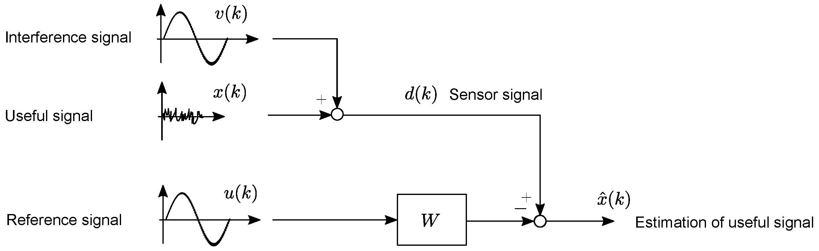
Further, the signal contains interference from power mains, i.e., it is deteriorated by harmonics of the mains frequency of 50 Hz. Thus, an interference canceling has to be implemented (see Figure 3). The sensor signal $d\left(k\right)$ is composed of a useful signal $x\left(k\right)$ and the interference $v\left(k\right)$. A reference signal $u\left(k\right)$ of the same frequency as the interference is generated. By applying an appropriate filter W with an impulse response $\underline{w}$, a signal can be obtained that cancels the interference in the sensor signal. The remaining signal $\widehat{x}\left(k\right)$ thus provides a good estimation of the useful signal:

$$\widehat{x}\left(k\right)=d\left(k\right)-\sum _{n=1}^N{\underline{w}}_{n}u(n-k).$$

(1)

To obtain the filter coefficients of the filter W, the time-discrete Wiener–Hopf equation can be solved:

$${\mathbf{R}}_{uu}\underline{w}={\underline{R}}_{ud},$$

(2)

where ${\mathbf{R}}_{uu}$ denotes the autocovariance matrix of the reference signal $u\left(k\right)$ and ${\underline{R}}_{ud}$ the vector of cross-covariance values of $u\left(k\right)$ and $d\left(k\right)$. For a single harmonic interference, a filter of order $N=2$ is sufficient.

In a further preprocessing step, data at constant rotation speed were extracted to not include the ramping up and down effects in the training data. Afterwards, measurements from both sensors were divided into snippets to create distinct samples for training and evaluation of the classifiers. An AE sample consists of 8000 consecutive values measured at a sampling rate of 390,625 values per second (20.48 ms per sample), while a vibration sample consists of 4096 values, which corresponds to one second of measuring. The resulting datasets with the vibration and AE snippets were complemented by the extracted rotation speed as an additional column. For each vibration or AE sample, the mean and standard deviation were calculated and were afterwards standardized using these values. From each standardized sample, the Fast Fourier Transformation (FFT) was calculated. For AE data, the frequency range between 512 and 50,000 Hz was extracted, and for the vibration data, the frequency range between 5 and 512 Hz was used. The previously calculated mean and standard deviation values were appended to the FFT-transformed samples and thereby created a feature vector for each sample. An additional scaling of all datasets to a feature range between 0 and 1 was conducted based on the range parameters of the stage 1 training dataset. As a result of the described preprocessing steps, the feature vector for each AE snippet comprises 1014 values while the feature vector of each vibration snippet comprises 2045 values.

2.3. Data Fusion Approach

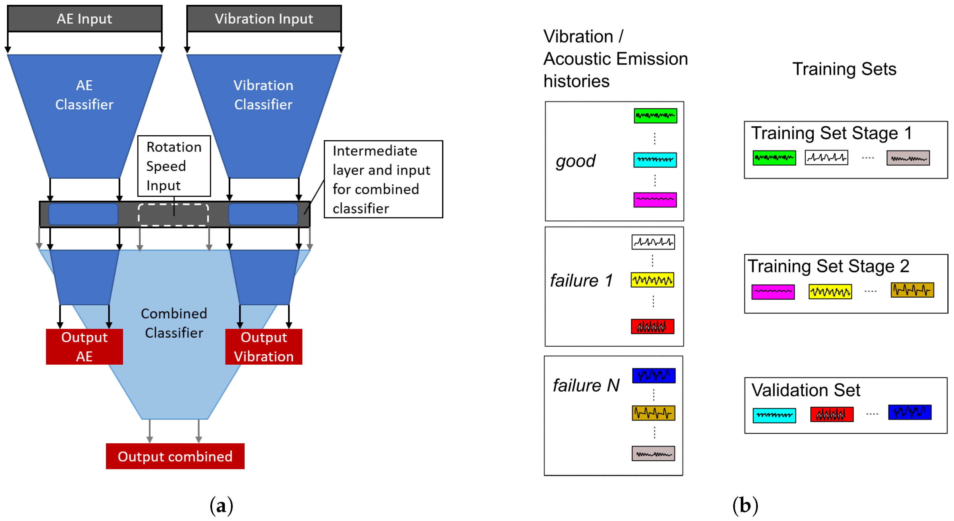
In this paper, a combined system is presented, which utilizes low-frequency vibration signals from accelerometers and high-frequency acoustic emission (AE) signals from ultrasonic transducers. By feeding the signals into a multi-stage classification algorithm (see Figure 4a), the capabilities of the detection should be enhanced to a broad range of faults and damages. The classifier architecture thereby consists of 3 parts, which are all trained to detect the defect state of the system:

• A classifier which receives data from the acoustic emission sensor (AE classifier);
• A classifier which receives data from the acceleration sensor (vibration classifier);
• A classifier which receives activations of the AE and vibration classifiers at intermediate layers (combined classifier) as well as the rotation speed.

The intention for this approach was to increase the sensitivity and to improve the resilience with respect to sensor failures. The proposed classifier architecture provides classifications based only on single sensor streams on the one hand (using the data from one sensor), and classifications based on fused sensor information on the other hand (using all available sensors). Thereby, sensitivity of the respective sensor data for the detection of different defect states can be evaluated and the performance gain due to the conducted sensor fusion can be assessed. Additionally, faults can even be detected if a single sensor stream is missing, albeit not with the maximum prediction accuracy.

In order to improve the training of the combined classifier, a stage 1 dataset and a stage 2 dataset were defined from the development dataset. An illustration of the splitting of the whole set of measurements into the stage 1 and 2 datasets as well as the validation dataset is depicted in Figure 4b. Like the validation dataset, the stage 2 dataset comprises one measurement per defect type and size. In an optimal configuration, the stage 2 dataset is only used to train the combined classifier, while the AE classifier and the vibration classifier are trained with the stage 1 dataset.

2.4. Classifier Setup

All the subclassifiers mentioned in Section 2.3 are multi-layer perceptrons. This type of neural network together with the frequency transformed input samples was chosen, since for vibration measurements it was shown that it can lead to classifiers with better generalization ability compared to, e.g., convolutional neural networks, which receive the time domain signals as an input [1]. The AE classifier has three hidden fully connected (dense) layers, each with 1024 nodes, and the vibration classifier has two hidden layers, also consisting 1024 nodes, respectively. Dropout was applied to all hidden layers of both classifiers to reduce overfitting. The combined classifier uses the activations of the last hidden layer of both the AE classifier and the vibration classifier as well as the scaled rotation speed as one concatenated input vector. In addition, it has two hidden layers, each with 128 nodes. No dropout was applied to the combined classifier since enough variability was induced by the intermediate layer values of the AE and vibration classifiers. The neural network was implemented using Tensorflow [42] and the used source code is documented at the corresponding Github repository [39]. Its layer architecture is depicted in Figure 5a.

During the training phase of the combined classifier, the weights of the AE classifier and the vibration classifier are frozen to only fit the weights of the combined classifier.

3. Results

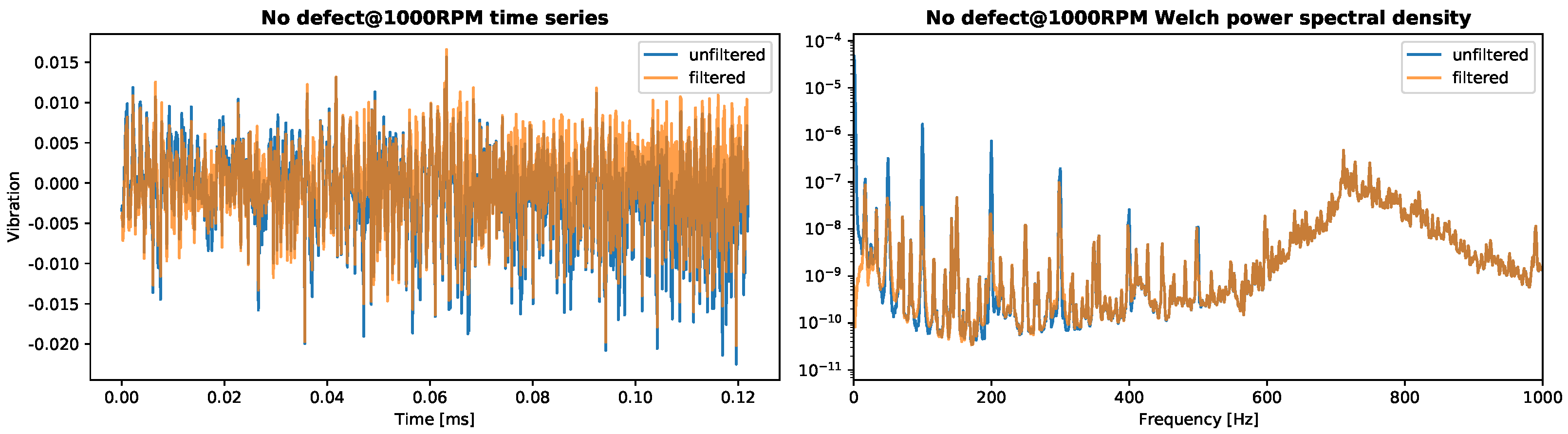
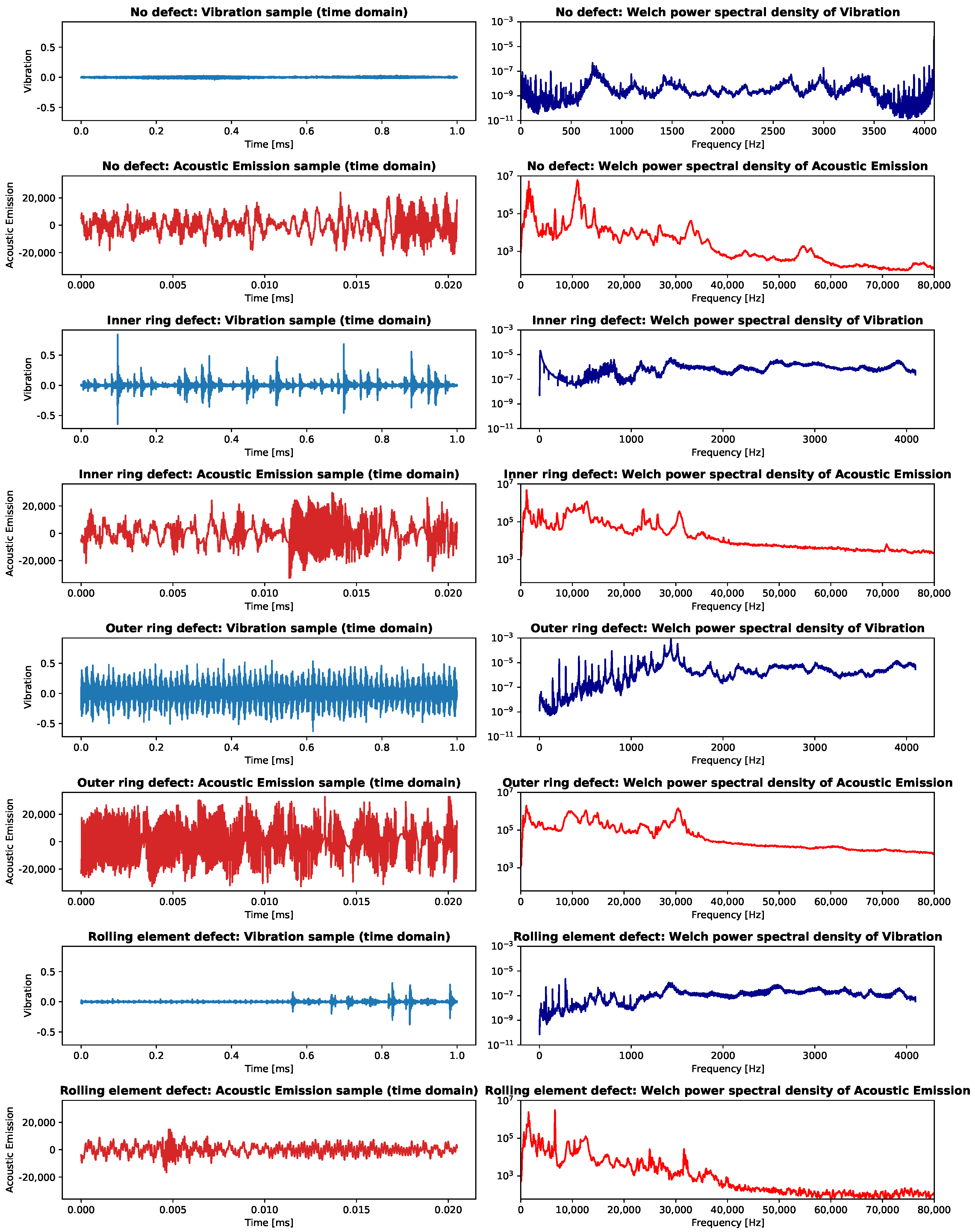
All vibration data were treated with the preprocessing and filtering as described above. The interference canceling was implemented successively for the frequencies 50, 100, 200, 300, 400 and 500 Hz. Figure 6 shows an example for a time series acquired in the undamaged state. Obviously, the Wiener filter with the reference signal suppressed only the interference while leaving the vibration signals from the bearing unaffected. An overview of the measured and preprocessed sensor time series as well as their transformation into the frequency domain are provided in Figure 7.

At first and as a baseline, both the AE and the vibration classifiers were trained on the full training dataset (including stage 1 and stage 2 training datasets). Each one acquired the scaled feature vectors from the respective sensor. Both classifiers achieved accuracies close to 100% on the training dataset. Classification results of the trained classifiers on the unseen validation dataset are visualized in Figure 8a,b. While both classifiers correctly or almost correctly classified the defect free measurement and the measurement with the damaged rolling element, they both failed to classify the measurement of the outer ring defect. The inner ring defect can be recognized by the AE classifier, while the vibration classifier is only partially able to correctly classify this measurement.

Here, we see a typical weak point of drive train CM systems: since the frequency spectra of single samples inside one measurement differ only slightly, it is a relatively easy task for any machine learning algorithm to recognize other samples from the same measurement. However, there are comparatively huge differences in frequency spectra between samples from different measurements, even when they belong to the same defect class and especially when the setup is dismantled and reassembled between the measurements, as was carried out here. It is therefore easier for the classifier to learn characteristic features of each measurement rather than to learn characteristic features of each defect state. A much larger number of measurements would be necessary to compensate for these effects and to achieve robust classifiers. An approach to increase the robustness of the defect state classification is to combine the information from both used sensor modalities. This is achieved by the proposed combined classifier. In a first experiment, the combined classifier is trained on the full training dataset. The pretrained vibration and AE classifiers thereby provide the input for the combined classifier. Their weights, however, remain unchanged during this procedure. In addition, the rotation speed is also an input to the combined classifier. The classification accuracies of the resulting classifier on the validation dataset are depicted in Figure 8c. Still, the outer ring defect cannot be classified correctly and the accuracy for the inner ring defect is not perfect. Again, the reason for this result is the overfitting of the vibration and AE classifiers. Since all classifiers receive input data from the same measurements, the combined classifier is not able to learn when to trust more the vibration classifier and in which cases the AE classifier is more reliable, because both of them are almost perfectly able to correctly classify samples from the dataset they are trained on.

To let the combined classifier learn when to trust which of the preclassifiers more, it needs to be trained with data from measurements unseen to the vibration and the AE classifiers. For this purpose, the splitting of the training dataset in the stage 1 and the stage 2 training datasets, as described in Section 2.3, was conducted. At first, the vibration classifier and the AE classifier were trained on data from the stage 1 training dataset. The combined classifier was afterwards fitted to data from the stage 2 training dataset. As with the validation data, both preclassifiers were not able to perfectly classify the measurements from the stage 2 dataset and therefore the combined classifier could learn when to trust which one more or less. The validation result of the combined classifier trained with the described procedure is shown in Figure 8d. A remarkable improvement in the classification accuracy is apparent, which indicates that the resulting classifier is much more robust to changing vibration behavior caused by a remounting of the setup compared to the classifier approaches discussed before.

4. Discussion and Outlook

Using the presented approach, bearing damages at drive trains can be detected early, precisely and robustly. While both sensor types enable a defect state classification separately, their data fusion further improves the fault detection sensitivity when they are trained on data from different measurements. On the other hand, in case of a sensor failure, a defect state classification can still be obtained since classifications are also calculated solely depending on one of the sensors at the same time. This is beneficial compared to the approaches reported in the literature (e.g., [3,34,37]), which only work when all sensor information is available. Still, it has to be considered that the predictions with partially missing sensor data lead to a lower accuracy compared to the case without sensor failure.

Comparisons in terms of fault detection accuracy are generally difficult to conduct since defect severity differs and also the experimental setups are not identical. Additionally, the division of the datasets into training, test and validation data differs significantly between the individual works. Many studies conduct a random train–test split between all the available data [3,22,27] as this is a common practice in the machine learning field. However, as stated above, vibration characteristics vary only slightly once a setup is completely assembled. As a result, almost perfect recognition accuracies can be achieved, while the classification algorithm used has only learned how a certain measurement can be identified, but does not have a correct internal representation of the error state. In an actual production facility, maintenance works are still necessary even when sophisticated CM systems are in place. During maintenance, screws may be replaced, lubricants may be refilled or adoptions due to changing products are necessary. These real-world conditions were simulated in this study by using independent measurements for model development and validation. In addition, the setup was dismantled and reassembled between each measurement, as explained in Section 2.1. The used algorithms for combining information, on the other hand, could be compared when applied to identical datasets. This work paves the way for a future comparative study by publishing the used dataset [43] as well as the used source code [39].

In a next step, the concept needs to be evaluated on a broader and continuous rotation speed range as well as with differently sized drive trains. A further limitation is that no load was used in this study. Investigations with varying loads could make the obtained dataset even more realistic. Additional sensor modalities (e.g., motor current, thermography) can increase the capabilities of the CM system further. Using a higher number of sensors in turn requires the development of algorithms with which the computational complexity can be reduced. Investigations need to be conducted that quantify the diagnostic information gain of each sensor for the defect state classification so that sensors that do not improve the detection capability of the system can be removed. Still, the data fusion concept presented here is not limited to AE and vibration data but is applicable for the fusion of many kinds of sensor time series, such as sound, temperature or pressure sensors. In particular, it is beneficial when a CM system needs to be resilient against sensor failures.