Role Reversals in a Tri-Trophic Prey–Predator Interaction System: A Model-Based Study Using Deterministic and Stochastic Approaches

Abstract

It is frequently observed that adult members of prey species sometimes use their predation mechanism on juvenile members of predator species. Ecological literature describes this phenomenon as prey–predator role reversal dynamics.Numerous authors have observed and described the biological development behind this feeding behaviour. However, the dynamics of this role reversal have hardly been illustrated in the literature in a precise way. In this regard, we formulated an ecological model using the standard prey–predator interactions, allowing for a reverse feeding mechanism. The mathematical model consisted of a three-species food-web structure comprising the common prey, intermediate predator, and top predator. Note that a role-reversal mechanism was observed between the intermediate and top predators based on the scarcity of the prey population. However, we observed the most critical parameters had a significant effect on this reverse feeding behaviour. The bifurcation analysis is the primary criterion for this identification. The proposed deterministic model is then extended to its stochastic analogue by allowing for environmental influences on the tri-trophic food web structure. The conditional moment approach is applied to obtain the equilibrium distribution of populations and their conditional moments in the system. The stochastic setup analysis also supports the stability of this food chain structure, with some restricted conditions. Finally, to facilitate the interpretation of our mathematical results, we investigated it using numerical simulations.

1. Introduction

In recent decades, the prey–predator relationship has been of great interest to all ecologists. Several authors [1,2,3,4,5] have conducted extensive work to capture all possible interactions between prey and predators. The most common aspect of the relationship is the general interactive dynamics, i.e., predator attacks, where the prey avoids predation. Apart from the general interaction, a special kind of relationship exists where prey reverse their feeding behavior for the predator species. The ecological literature describes this phenomenon as prey–predator role reversal dynamics. Although there are several paradigms of predatory dynamics in our ecosystem, like intraguild predation [6] and predation due to the switching mechanism [3,4], it is frequently observed that the adult of the prey species sometimes shows their predation mechanism on the juvenile predator. Numerous authors have witnessed and explained the biological development behind this reversed dynamic [7,8,9,10], but extensive mathematical modelling is still needed to explore the inherent dynamics of the role-reversal mechanism in a better way.

A novel work in the domain of predator–prey role reversal was conducted by Barkai and McQuaid [10]. The authors identified first the role reversal phenomena on the Malgas Island of South Africa, between a decapod crustacean (Jasus lalandii) and a marine snail (Burnupena papyracea). The rock lobster Jasus lalandii was generally found to exert its predatory behaviour on Burnupena papyracea. However, it was observed that sometimes the crustacean’s juvenile members were predated by the adult whelks. Consequently, the abundance of the predatory species, i.e., the crustacean J. lalandii, was expected to go extinct at some point in time. The authors Barkai and McQuaid [10] performed a controlled ecological experiment on that island to rescue the population of J. lalandii, so that an equilibrium was maintained in that marine ecosystem. Fauchald [11] also elicited the role reversal dynamics between the Atlantic cod (Gadus morhua) and the Atlantic Herring fish (Clupea harengus) in the northern-shelf ecosystems where cod predated upon herring fish. The overfishing effect of G. 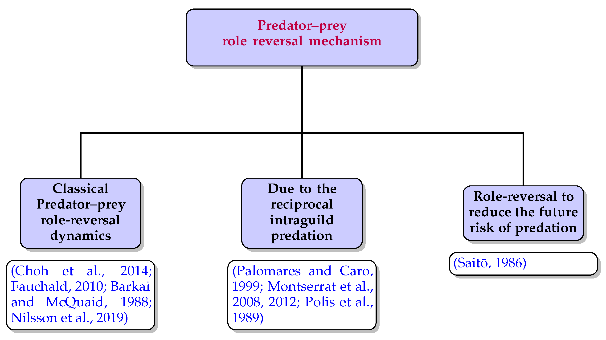morhua for economic purposes is another reason for their population decline [12]. The convolution of the role reversal dynamics and the overfishing effect is responsible for the “ecosystem hysteresis” in that northern-sea region. Based on the paradigms mentioned earlier, the role reversal dynamics can be classified into three categories, i.e., (a) the classical role-reversal mechanism; (b) role reversal due to reciprocal intraguild predation; and (c) role-reversal for reducing only the future predation risk. The works discussed by the authors of [10,11] described the classical predator–prey role-reversal mechanism. Seminal experimental works were also performed by the authors of [9,13] to demonstrate the classical predator–prey role-reversal action. Reciprocal intraguild predation is defined as the interspecific killing of juvenile family members by the adult member of those predators for the competition of the resources [14]. The predation of the predator family’s juvenile offspring by the adult member of the same species is responsible for the reverse feeding behaviour [15,16,17]. In this regard, Palomares and Caro [17] provided a pattern in their research article demonstrating the interspecific killing among carnivores. The pattern captures all possible interactions between the juvenile and adult members of the same carnivorous species. The third category of the role reversal dynamics revealed that sometimes the prey family’s adult member only eradicates the predator’s juvenile member, but does not consume them. Saito [18] demonstrated the third category through performing a biological experiment between the spider mite prey Schizotetranychus celarius and their phytoseiid mite predator Typhlodromus bambusae. The author concluded that the immobile nature of the phytoseiid mite’s egg was one reason behind this type of killing and explained the incident as an “arms race” between the prey and the predator to reduce the future risk of predation. The three categorizations are also expressed through the flow diagram (see Figure 1).

Most experimental work in the role reversal domain is based on the first category. One of the important aspects of the classical category is the work of Choh et al. [6]. The main theme behind the research is that the predation experience of the survived juvenile prey during their exposure to the predator interaction acts as a major yardstick for the reverse attack on the juvenile predator during the adult stage of the prey that survived. Choh et al. [6] claimed that the boldness and aggressiveness of some juvenile prey is the key regulator for their lower predation risk for other prey species. The author carried out this experiment by considering the following three predatory (mite) species, i.e., Iphiseius degenerans (Berlese), Neoseiulus cucumeris (Oudemans), and Amblyseius swirskii (Athias-Henriot) (Acari: Phytoseiidae). The three mite species are predated on by small insects and pollens derived from the plants. However, the adults and juveniles of I. degenerans and N. cucumeris predated on the infant stages of the other species, with adult members attacking juvenile ones, even when the substitute food (such as pollen) is available [15]. Choh et al. [7] also ensure that the prey species’ ontogenetic development may be another reason behind the reverse feeding behaviour. Breton and Addicott [19] also documented the reverse feeding action as the mutualistic behaviour between the prey–predator.

Despite its significance, most ecologists have ignored the role reversal issue. The importance of the role reverse mechanism lies in the interaction between prey and predators and how this impacts the stability of any ecosystem. Sanchez-Garduno et al. [20] and Lehtinen [21] are some of the authors who have incorporated role reversal dynamics into their modeling structures. The seminal work of Sanchez-Garduno et al. [20] is based on the interaction between two predatory species that do not have any common prey. The recent publication of Lehtinen [21] also described the reverse feeding action in a platform of a two-dimensional model. Lehtinen [21] assumed several conditions, like prey hiding and cannibalism, to describe his work. Moreover, the author was more interested in predator extinction by incorporating the Allee effect phenomena. As a consequence, the novelty of the role reversal mechanism has been ruled out from both of these works. In light of this, there is an urgent need to construct a proper mathematical model that can describe the reverse feeding mechanism in a precise way.

Engen et al. [22] describes that the ecological state of any system can be understood through the model parameters, but the implication of model parameters in the work of Sanchez-Garduno et al. [20] is not properly mentioned. The sensitivity of any parameter is always responsible for both the stability and instability of any ecological system [3], which is missing in the studies of Sanchez-Garduno et al. [20] and Lehtinen [21]. Moreover, ecosystems are open systems, so the environment’s involvement is seriously reliant on ecological scenarios. An ecological system’s deterministic stability does not guarantee that an equilibrium will be established in any random environment [23]. Sanchez-Garduno et al. [20], Lehtinen [21] also ignored the effect of natural calamities in their modeling structure, despite the fact that all ecological interactions are intertwined with natural processes. It has been argued the creation of predictive models of role-reversal interactions will greatly alleviate efforts towards preventing ecological collapse or understanding alternative ecosystem states under changing conditions [20].

However, the impact of the reverse feeding (role reversal) mechanism on the interactive dynamics between prey and their predators for shaping an ecosystem has been less explored. Although there are some empirical studies that have been conducted in this regard, in mathematical modeling of an ecological system, there is much less research. This, however, creates a gap in understanding the effect of the role-reversal mechanism on the conspecific interaction between prey and predators in an ecosystem. So, in a nutshell, maintaining the aspects of several experiments [6,10,18] and in the spirit of Sanchez-Garduno et al. [20] and Lehtinen [21], we provide a new mathematical overlay to the predator–prey role reversal dynamics. By employing this modeling approach, which depicts a three-species food-web structure, the influence of the role reversal mechanism on the interactive dynamics between the prey and their predator becomes more clearly apparent than in other empirical studies. This model includes common prey—intermediate or mesopredator—along with a top predator. The top predator predates both the common prey and the intermediate predator; but, based on circumstantial evidence, the intermediate predator reverses its feeding role. The modeling structure also addresses the involvement of the environment in ecological interactions to develop a better ecological understanding. Based on this, we summarize our manuscript in the following way, i.e., Section 2 is devoted to the discussion of the model formulation with the ecological synergy and persistence, permanence, and related dynamical behavior of our proposed model system (5). In Section 3, we describe the interplay between the top and intermediate predator through the sub-model (6), along with the corresponding model analysis. We discuss the extension of the proposed deterministic role-reversal model to its stochastic analogue using stochastic differential equations (SDEs) in Section 4. The results of our analytical findings are discussed in the context of biological realization in Section 5. Finally, the paper ends with a conclusion in Section 6. For ease of reading, some analytical calculations and proofs are shown in the Supplementary Material.

2. Model Formulation

The main objective behind the development of this section is to create a proper mathematical understanding so as to quantify the role reversal dynamics concerning the species’ feeding behavior. Several paradigms are present, which demonstrate that, based on the feeding behavior of any species, it can reverse their role in the ecosystem [7]. Based on the aforementioned evidence, we propose a deterministic growth model describing the role reversal dynamics between more than one species. For the sake of simplicity, we considered a three-species food web where one species acts as the prey and the remaining two are the predators of that prey species. We further classified the predator species into two subgroups, i.e., the intermediate predator and the top predator. The superpredator (or the top predator) can feed on both the intermediate predator and prey, whereas the intermediate predator shows their predatory behavior on the prey only. However, the scarcity in the prey population and the predation risk sometimes compel the intermediate predator to reverse their feeding role. It is evident that the risk factor enables the intermediate predators’ adult members to predate the juvenile member of the top predator [7]. According to [3], one of the most important roles in a tri-trophic food-chain system is that of the intermediate predator, which is responsible for regulating the system’s stability.

Keeping these aspects in mind, we developed a three-species food chain model. Here, the prey population is denoted by $R\left(t\right)$; in the absence of any predator, the prey species is considered to grow logistically with an intrinsic growth rate of r and with K as their carrying capacity. The carrying capacity is the maximum population size of any system. So, the growth rate profile for the prey species can be expressed as

$$\frac{dR\left(t\right)}{dt}=rR\left(t\right)\left(1-\frac{R\left(t\right)}{K}\right)$$

(1)

As two predatory species are present in the food-web structure, their predation on the prey should profoundly affect the growth of the prey species. In ecological literature, the prey species’ predatory behavior is captured through the “functional response” term. The functional response is described as the rate at which a predator captures any prey. It would be expected that the relationship between the functional response and the prey density would increase linearly. However, in most of the evidence, for a substantial amount of prey density, the predator should be limited by the handling time and the time taken to consume the prey [3,24,25]. Considering both of these aspects, Holling [25] proposed a functional relationship for the predator’s response on the prey, popularly known as the “Holling type-II functional response”. The fundamental assumption behind the construction of the response function is that upon increasing the prey density, the magnitude of the response function increases very much. Still, because of the effect of predator satiation, the magnitude of the response function would be unaltered after a certain threshold amount of prey density. Mathematically, this type of function is demonstrated through the hyperbolic function. It is sometimes referred to as the hyperbolic response function, as the prey is abundant in the system. We can also demonstrate the interaction between the prey and predators through the “Holling type-II functional response” function.

As discussed above, we considered both the intermediate and top predators as the two other species in the food chain. So, both of them interact with the prey. Now, the assumption of a small prey size and the dynamics of both the adult and juvenile members of the top predator highlights the feeding action of both the juvenile and adult members of the top predator. In this regard, we consider that the transition rate of the juveniles to the adult stage is b, with its magnitude lying in the semi-closed interval $[0,1)$. It is evident from the interactive dynamics of some species that the juvenile member of the top predator predates the prey. Based on this event, we consider the response function as $\frac{{\alpha }_{2}R\left(t\right)(1-b)P\left(t\right)}{{\beta }_2+R\left(t\right)}$, with ${\alpha }_2$ and ${\beta }_2$ as the catching rate and half-saturation constant, respectively, and $P\left(t\right)$ as the density of the super-predator. As the prey species is the basal food source of the intermediate predator, all members must predate the prey species extensively. In this regard, the analytic expression of the functional response between the prey and the intermediate predators should be $\frac{{\alpha }_{1}R\left(t\right)N\left(t\right)}{{\beta }_1+R\left(t\right)}$, with $N\left(t\right)$ as the density of the intermediate predator. Thus, the complete growth function of the prey species is represented by

$$\frac{dR\left(t\right)}{dt}=rR\left(t\right)\left(1-\frac{R\left(t\right)}{K}\right)-\frac{{\alpha }_{1}R\left(t\right)N\left(t\right)}{{\beta }_1+R\left(t\right)}-\frac{{\alpha }_{2}R\left(t\right)(1-b)P\left(t\right)}{{\beta }_2+R\left(t\right)}$$

(2)

Predator–prey relationships are often perceived simply as situations in which a predator enhances its fitness by reducing its prey’s fitness. The predation effect of the intermediate predator decreased the prey abundance. Similarly, predatory behavior also helps their growth. So, the component of predation plays a positive role in the growth of the intermediate predator, which is captured through the same response function between the prey and intermediate predator, i.e., $\frac{e_1{\alpha }_{1}R\left(t\right)N\left(t\right)}{{\beta }_1+R\left(t\right)}$ where $e_1$ is denoted as the rate of conversion of the consumption of the prey into the growth of the intermediate predator. However, the relationship between the intermediate predator and the top predator may become reversed when the intermediate predator feeds on the juvenile member of the top predator [7].

It is frequently observed that during reverse feeding behavior, the juvenile members from the top predator families are abundant in the ecosystem [14]. So, it becomes convenient to find the prey species (juvenile members of the top predator) for the intermediate predator. This clearly specifies that the interaction between the juvenile prey and the predator should be proportional to their population density, which can be better explained by the principle of mass action [20,21]. Note that the Holling type-I equation is the best function to express this scenario [26]. So, we modified the type-I response function to explain the reverse feeding action. The analytical form of this function is provided by $e_2{\alpha }_{4}aN\left(t\right)(1-b)P\left(t\right)$, with ${\alpha }_4$ and $e_2$ denoting the predation rate and consumption rate of the intermediate predator, respectively. This consumption behavior helps the intermediate predator with their growth, and, in a similar way, the predation of the intermediate predator reduces the density of the top predator extensively. As both the intermediate and top predator coexist simultaneously, an intra and inter-specific competition must be present between the species. The inter-specific competition is reflected through the above functional response term. But, there remains a competition for the resources between the intermediate and top predator species, namely intra-specific competition. We assume that the intraspecies competition acts as a precursor of species extinction in a population of multi-species food-web model [3]. Similarly, we also considered the natural death of the intermediate predator to establish an equilibrium in any ecosystem. This means that the intermediate predator’s mortality rate consists of two components: (i) death due to the intraspecies competition and (ii) natural death. Motivated by the concept of the logistic growth law, we also considered the mortality rate as $N\left(t\right)\left({\gamma }_{1}N\left(t\right)-d_1\right)$. Hence, the complete growth equation of the intermediate predator is provided by

$$\frac{dN\left(t\right)}{dt}=\frac{e_1{\alpha }_{1}R\left(t\right)N\left(t\right)}{{\beta }_1+R\left(t\right)}-\frac{{\alpha }_{3}N\left(t\right)bP\left(t\right)}{{\beta }_3+N\left(t\right)}-{\gamma }_1{N}^2\left(t\right)+e_2{\alpha }_{4}aN\left(t\right)(1-b)P\left(t\right)-d_{1}N\left(t\right)$$

(3)

The top predator’s growth rate function similarly consists of the growth and the mortality term, respectively. The growth function of the top predator is the convolution of the two predation concepts. One is predation of the juvenile member on the prey species, and the other is predation of the adult member on the intermediate predator. So, the analytic expression of the growth term is provided by $\frac{e_3{\alpha }_{2}R\left(t\right)(1-b)P\left(t\right)}{{\beta }_2+R\left(t\right)}+\frac{e_4{\alpha }_{3}N\left(t\right)bP\left(t\right)}{{\beta }_3+N\left(t\right)}$. Concurrently, the top predator’s mortality function consists of three components, i.e., mortality due to the species’ intraspecific competition, natural death rate, and the consumption of the juvenile member of the top predator by the intermediate predator. The analytic expression of the death term is provided by ${\gamma }_2{P}^2\left(t\right)-{\alpha }_{4}aN\left(t\right)(1-b)P\left(t\right)-d_{2}P\left(t\right)$. So, the growth rate of the top predator can be expressed as

$$\frac{dP\left(t\right)}{dt}=\frac{e_3{\alpha }_{2}R\left(t\right)(1-b)P\left(t\right)}{{\beta }_2+R\left(t\right)}+\frac{e_4{\alpha }_{3}N\left(t\right)bP\left(t\right)}{{\beta }_3+N\left(t\right)}-{\gamma }_2{P}^2\left(t\right)-{\alpha }_{4}aN\left(t\right)(1-b)P\left(t\right)-d_{2}P\left(t\right)$$

(4)

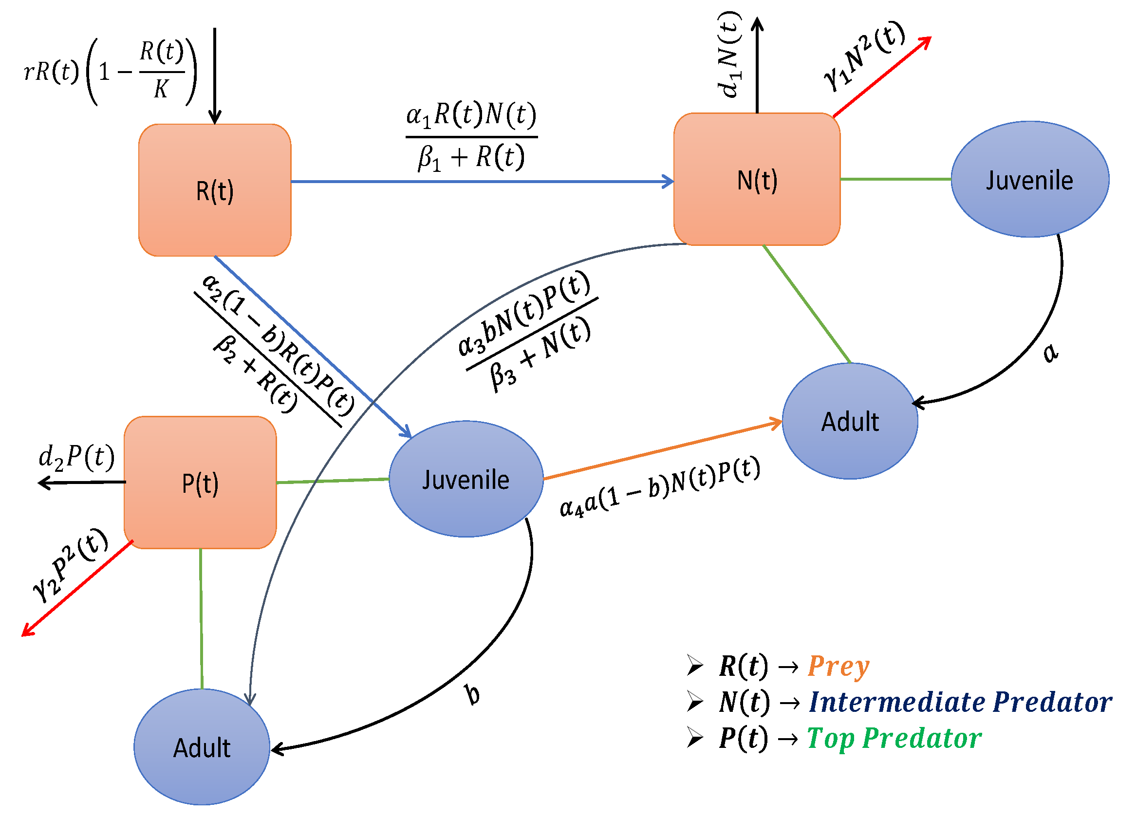
Combining all these relationships (2)–(4), the complete food web model is given by

$$\begin{array}{c}\hfill \left.\begin{array}{c}\frac{dR\left(t\right)}{dt}=rR\left(t\right)\left(1-\frac{R\left(t\right)}{K}\right)-\frac{{\alpha }_{1}R\left(t\right)N\left(t\right)}{{\beta }_1+R\left(t\right)}-\frac{{\alpha }_{2}R\left(t\right)(1-b)P\left(t\right)}{{\beta }_2+R\left(t\right)}\hfill \\ \\ \frac{dN\left(t\right)}{dt}=\frac{e_1{\alpha }_{1}R\left(t\right)N\left(t\right)}{{\beta }_1+R\left(t\right)}-\frac{{\alpha }_{3}N\left(t\right)bP\left(t\right)}{{\beta }_3+N\left(t\right)}-{\gamma }_1{N}^2\left(t\right)+e_2{\alpha }_{4}aN\left(t\right)(1-b)P\left(t\right)-d_{1}N\left(t\right)\hfill \\ \\ \frac{dP\left(t\right)}{dt}=\frac{e_3{\alpha }_{2}R\left(t\right)(1-b)P\left(t\right)}{{\beta }_2+R\left(t\right)}+\frac{e_4{\alpha }_{3}N\left(t\right)bP\left(t\right)}{{\beta }_3+N\left(t\right)}-{\gamma }_2{P}^2\left(t\right)-{\alpha }_{4}aN\left(t\right)(1-b)P\left(t\right)-d_{2}P\left(t\right)\hfill \end{array}\right\}\end{array}$$

(5)

The above discussion is also outlined in the schematic diagram in Figure 2. Here, the compartments of juvenile and adult were created for better representation. The description of state variables and parameters along with their ecological meaning of the model system (5), are shown in

Table 1. Ecological description of variables and parameters used in the system (5).

Variables
&	Ecological Meaning
Parameters
$R\left(t\right)$	Population density of prey
$N\left(t\right)$	Population density of intermediate predator
$P\left(t\right)$	Population density of top predator
r	Intrinsic growth rate of prey
K	Environmental carrying capacity of prey
${\alpha }_1$ and ${\alpha }_2$	Consumption rate of prey by each intermediate predator and juvenile member of top predator in unit time
${\beta }_1$ and ${\beta }_2$	Prey half saturation constant
a	Transition rate of intermediate predator from juvenile to adult stage with $a\in [0,1)$
b	Transition rate of top predator from immature to mature stage with $b\in [0,1)$
$e_1$	Conversion factor from prey to intermediate predator
${\alpha }_3$	Consumption rate of adult top predator to adult intermediate predator in unit time
${\beta }_3$	Adult intermediate predator half saturation constant
${\gamma }_1$ and ${\gamma }_2$	Intraspecific competition coefficient of intermediate predator and top predator
$e_3$	Conversion factor from prey to juvenile member of top predator
${\alpha }_4$	Consumption rate of adult intermediate predator to juvenile top predator
$d_1$ and $d_2$	Mortality rate of intermediate predator and top predator
$e_2$	Conversion factor from immature top predator to mature intermediate predator
$e_4$	conversion factor from mature intermediate predator to mature top predator

.

2.1. Positivity and Boundedness

Theorem 1. 

All possible solutions of the system (5) with the corresponding initial conditions always remain and bounded in the interior of ${\mathbb{R}}_{+}^3$.

Proof. 

The proof is given in the Supplementary Material. □

2.2. Persistence and Permanence

Persistence (or permanence) is the intricate property of any dynamical system. It addresses the long-term behavior of the concerned system, while permanence deals with the limits of growth for some of the system’s components. Permanence assures that the populations will recover from the infrequent disturbances often experienced by ecological systems [27]. Mathematically, persistence and permanence can be described as:

Persistence: 

The n dimensional dynamical system is said to be persistent if for any forward trajectory $T\left(c_0\right)=\{c\left(t\right)=\left(x_1\left(t\right),x_2\left(t\right),\dots ,x_n\left(t\right)\right)|t\ge 0\}$ with a positive initial condition $c_0\in R_{>0}^n$ we have ${lim}_{t\to \infty }inf{x}_i\left(t\right)>0\forall i\in \{1,2,\dots ,n\}$. Here, $R_{>0}$ is the set of strictly positive real numbers and for any integer $n>1$, we call $R_{>0}^n$ the positive orthant.

Permanence: 

The n-dimensional dynamical system is said to be permanent on a forward invariant set $D\subset R_{>0}^n$, where $R_{>0}^n$ be the positive orthant for any integer $n>1$ if ∃$ϵ>0$ such that for any forward trajectory $T\left(c_0\right)$ with a positive initial condition $c_0\in D$, we have $ϵ<{lim}_{t\to \infty }inf{x}_i\left(t\right)$ and ${lim}_{t\to \infty }sup{x}_i\left(t\right)<\frac{1}{ϵ}$.

Theorem 2. 

The proposed model system (5) is persistent under the following conditions.

(i) 

$r-{\alpha }_1{M}_N^{*}-{\alpha }_2(1-b)M_P^{*}>0$,

(ii) 

$\frac{e_1{\alpha }_1{m}_R}{{\beta }_1+K}-{\alpha }_{3}b{M}_P^{*}-d_1>0$,

(iii) 

$\frac{e_3{\alpha }_2(1-b)m_R}{{\beta }_2+K}+\frac{e_4{\alpha }_{3}b{m}_N}{{\beta }_3+M_N^{*}}-{\alpha }_{4}a(1-b)M_N^{*}-d_2>0$

Proof. 

The proof is present in the Supplementary Material. □

Theorem 3. 

The system (5) is said to be permanent if ∃ positive constants m and M, with $0<m\le M$ such that

$$min\{\underset{t\to \infty }{lim\; inf}R\left(t\right),\underset{t\to \infty }{lim\; inf}N\left(t\right),\underset{t\to \infty }{lim\; inf}P\left(t\right)\}\ge m$$

and

$$max\{\underset{t\to \infty }{lim\; sup}R\left(t\right),\underset{t\to \infty }{lim\; sup}N\left(t\right),\underset{t\to \infty }{lim\; sup}P\left(t\right)\}\le M$$

for all solutions $\left(R\left(t\right),N\left(t\right),P\left(t\right)\right)$ of the model system (5) with positive initial values.

Proof. 

The proof is present in the Supplementary Material. □

2.3. Equilibrium Points and Their Stability

The equilibrium point or the stationary point in an ecological system is defined as those points where the absolute growth velocity of the species vanishes. In our proposed model (5), six such cases arise, i.e., (i) the trivial equilibrium point $E_0$, (ii) predator-free (axial) equilibrium point $E_1$, (iii) top predator-free (planar) equilibrium point $\overline{E}$, (iv) intermediate predator-free (planar) equilibrium point $\widehat{E}$; (v) prey-free (planar) equilibrium point $\tilde{E}$, and (vi) coexisting equilibrium point $E^{*}$. A detailed description of the equilibrium points are provided in Supplementary Material.

Stability Analysis

The intricate property of any ecological or dynamical system is to maintain its stability. Equilibrium points are the static point, so they do not provide any insight into the influence of the other activities in any ecosystem. The inert nature of any ecological system will not always be perpetual, which means a dynamic flow is inevitable in that system. It is essential to nurture the behavior of the stationary points for that concerned system. The stability analysis of those equilibrium points would be the only way to serve this purpose. Our proposed model (5) also contains the six equilibrium points, so it is ubiquitous to analyze the stability of those six stationary points with respect to the corresponding prey–predator system. In this regard, we propose the following theorems to examine the stability of our proposed system (5).

Theorem 4. 

For the system (5),

•

Trivial equilibrium $E_0$ is always unstable.

•

Predator-extinction equilibrium $E_1$ is locally asymptotically stable if the following conditions hold:

${\alpha }_1<\frac{d_1}{e_1}\left(\frac{{\beta }_1}{K}+1\right)$ and ${\alpha }_2<\frac{d_2}{e_3(1-b)}\left(\frac{{\beta }_2}{K}+1\right)$.

•

Top-predator-extinction equilibrium $\overline{E}$ is locally asymptotically stable if $\left(\frac{2r\overline{R}}{K}+\frac{{\alpha }_1{\beta }_1\overline{N}}{{\beta }_1+\overline{R}}+2{\gamma }_1\overline{N}+d_1\right)>\left(r+\frac{e_1{\alpha }_1\overline{R}}{{\beta }_1+\overline{R}}\right)$, $\frac{e_1{\alpha }_1^2{\beta }_1\overline{R}\overline{N}}{{({\beta }_1+\overline{R})}^3}>\left\{\frac{{\alpha }_1{\beta }_1\overline{N}}{{\beta }_1+\overline{R}}+r(\frac{2\overline{R}}{K}-1)\right\}\left\{\frac{e_1{\alpha }_1\overline{R}}{{\beta }_1+\overline{R}}-(2{\gamma }_1\overline{N}+d_1)\right\}$ and ${\alpha }_4>{\alpha }_4^{*}$ (= threshold value of ${\alpha }_4$).

•

Intermediate predator-extinction equilibrium $\widehat{E}$ is locally asymptotically stable if the following conditions hold:

${\alpha }_3>\frac{{\beta }_3}{b\widehat{P}}\left\{\frac{e_1{\alpha }_1\widehat{R}}{{\beta }_1+\widehat{R}}+e_2{\alpha }_{4}a(1-b)\widehat{P}-d_1\right\}={\alpha }_3^{*}$ (= threshold value of ${\alpha }_3$) and $tr\left(B\right)<0$ and $det\left(B\right)>0$.

•

Prey-extinction equilibrium $\tilde{E}$ is locally asymptotically stable if $r<\frac{{\alpha }_1\tilde{N}}{{\beta }_1}+\frac{(1-b){\alpha }_2\tilde{P}}{{\beta }_2}$ and $tr\left(C\right)=(D_1+D_4)<0$ and $det\left(C\right)=(D_1{D}_4-D_2{D}_3)>0$.

Proof. 

The whole analytical work is provided in the Supplementary Material. □

Theorem 5. 

The coexisting equilibrium point ($E^{*}$) is locally asymptotically stable if ${\xi }_1>0$, ${\xi }_3>0$ and ${\xi }_1{\xi }_2-{\xi }_3>0$, where ${\xi }_1$, ${\xi }_2$ and ${\xi }_3$ are the coefficients of the characteristic equation of the Jacobian matrix ${\left[J\right]}_{E^{*}}$, which is ${\lambda }^3+{\xi }_1{\lambda }^2+{\xi }_2\lambda +{\xi }_3=0$.

Proof. 

The analytical calculation is provided in Supplementary Material. □

Furthermore, system (5) may undergo Hopf bifurcation if ${\xi }_1{\xi }_2-{\xi }_3=0$ holds.

It is worthwhile to note that the stability conditions of the coexisting equilibrium $E^{*}$ are very complicated. Consequently, it is difficult to explain the biological meaning of such mathematical expressions. We use numerical computations to verify and illustrate the stability of the prey, intermediate predator, and top predator. Figure 3 shows the local stability of the system (5) around the interior equilibrium point $\left(E^{*}\right)$. It is noted that the parametric values are mentioned in the figure caption. Figure 4 shows the global stability of the system (5) at $E^{*}$ for different initial conditions and the other parametric values are mentioned in the corresponding figure caption.

Theorem 6. 

The positive coexisting equilibrium $E^{*}(R^{*},N^{*},P^{*})$ is globally asymptotically stable with respect to all the solutions initiating in the interior of ${\mathbb{R}}_{+}^3$ if the following conditions hold:

(i) 

$e_2>1$,

(ii) 

$e_1>1$ and $A^{\prime }<{\beta }_1(e_1-1)$,

(iii) 

$\frac{A^{\prime }}{K}>\frac{{\alpha }_{1}B}{({\beta }_1+A^{\prime })({\beta }_1+R^{*})}$

Proof. 

The proof is provided in the Supplementary Material. □

2.4. Bifurcation Analysis of Main Model

The stability of any ecosystem does not always depend on its dynamic movement, rather it also sometimes relies on the intrinsic growth behavior of the species. The underlying growth actions of any species should be extensively judged through the model parameters involved in that ecosystem [22]. It is evident that certain changes in the model parameters result in disturbances in the stability of the corresponding ecosystem [3,5]. The efficacy of the bifurcation analysis is too structured to demonstrate the issue. The bifurcation of any system is defined as the qualitative change in the behavior of the equilibrium points when changing the parameter values. The selection of the model parameter as the bifurcation parameter is one of the important aspects from an ecological point of view. Here, we select the transition rate, a and b, of the intermediate and top predator, respectively, as bifurcation parameters because the prey shifts from being prey to a predator when it transitions from the juvenile to adult stage. For the predators, the scenario is different as they are always the predator during the adult stage, but during the juvenile stage, they are the victims (prey) of the adult prey.

Theorem 7. 

The necessary and sufficient condition for the occurrence of Hopf bifurcation of the system (5) at $b=b^{*}$ are

(i) 

${\xi }_i\left(b^{*}\right)>0$ for $i=1,2,3$ and ${\xi }_1\left(b^{*}\right){\xi }_2\left(b^{*}\right)-{\xi }_3\left(b^{*}\right)=0$

(ii) 

$Re{\left[\frac{d{\lambda }_i}{db}\right]}_{b=b^{*}}\ne 0$ for $i=1,2,3$

where ${\lambda }_i$ are the roots of the characteristic equation corresponding to the coexisting equilibrium point $E^{*}$.

Proof. 

The proof is provided in the Supplementary Material. □

Remark 1. 

In a similar manner, we check that Hopf bifurcation also occurs with respect to the transition rate $\left(a\right)$ of intermediate predator from the juvenile to adult stage.

3. Interplay between the Top and Intermediate Predators

Ecological literature depicts that in any tri-trophic food-chain system, the intermediate predator tends to change their role from prey to predator with respect to the top predator, due to a lack of prey or to reduce the predation risk. Although biologists routinely assign the species as prey or predator, there is sometimes no conspicuous winner, as prey can sometimes predate or inflict harm on their predators. This indicates that cyclic dominance is also noteworthy for prey–predator interactions. Indeed, role reversal between prey and predators is an evolutionary adaptation developed over time, which collaborates prey organisms in their constant struggle against their predators.

It is well documented that prey can reduce predation risk in several ways, such as through behavioral changes. Role reversals or exchanges of roles are a more common occurrence in interactive dynamics than what was once believed. In prey–predator interactions, a species’ ecological roles may change during development, from the earliest stage to maturity. It is also observed, depending on the scarcity of the prey population, that the middle or intermediate predator will switch their predation behavior on the juvenile member of the top predator. The prey–predator reversal is a biological interaction in which a species plays the role of predator in the prey–predator interaction rather than functioning as the usual prey. In population ecology, it is infrequently observed that a species act as prey during its juvenile stage and may become a predator in their adult stage [7,9,11]. In this context, it is essential to analyze the dynamics between the middle and top predators. We considered the following sub-model from the proposed system (5).

$$\begin{array}{c}\hfill \left.\begin{array}{c}\frac{dN\left(t\right)}{dt}=e_2{\alpha }_{4}aN\left(t\right)(1-b)P\left(t\right)-\frac{{\alpha }_{3}N\left(t\right)bP\left(t\right)}{{\beta }_3+N\left(t\right)}-{\gamma }_1{N}^2\left(t\right)-d_{1}N\left(t\right)\hfill \\ \\ \frac{dP\left(t\right)}{dt}=\frac{e_4{\alpha }_{3}N\left(t\right)bP\left(t\right)}{{\beta }_3+N\left(t\right)}-{\gamma }_2{P}^2\left(t\right)-{\alpha }_{4}aN\left(t\right)(1-b)P\left(t\right)-d_{2}P\left(t\right)\hfill \end{array}\right\}\end{array}$$

(6)

with non-negative initial conditions $N\left(0\right)>0$ and $P\left(0\right)>0$. The notations were the same with the system (5). The above discussion is also outlined in the following schematic diagram (see Figure 5). Note that in this flow diagram, we create the compartment of juvenile and adult for better convenience.

3.1. Analysis of Sub-Model

In this segment of the analysis, we are considered a situation where both the intermediate predator $\left(N\right(t\left)\right)$ and top predator $\left(P\right(t\left)\right)$ coexisted simultaneously and could live together in a diverse environment. So, we considered only the interior equilibrium $\left(E_s^{*}\right)$ of the sub-model (6).

Theorem 8. 

The interior equilibrium point $E_s^{*}(N_s^{*},P_s^{*})$ is locally stable if ${\mu }_1>0$ and ${\mu }_2>0$.

Proof. 

The characteristic equation of the Jacobian matrix $J\left(E_s^{*}\right)$ is provided by

$$\begin{array}{c}\hfill {\lambda }^2+{\mu }_1\lambda +{\mu }_2=0\end{array}$$

where ${\mu }_1=-(Q_{11}+Q_{22})$ and ${\mu }_2=Q_{11}{Q}_{22}-Q_{12}{Q}_{21}$

$$\begin{array}{ccc}\hfill Also,& Q_{11}=e_2{\alpha }_{4}a(1-b)P-\frac{{\alpha }_3{\beta }_{3}bP}{{({\beta }_3+N)}^2}-2{\gamma }_{1}N-d_1\hfill & \\ & Q_{12}=e_2{\alpha }_{4}a(1-b)N-\frac{{\alpha }_{3}bN}{{\beta }_3+N}\hfill & \\ & Q_{21}=\frac{e_4{\alpha }_3{\beta }_{3}bP}{{({\beta }_3+N)}^2}-{\alpha }_{4}a(1-b)P\hfill & \\ & Q_{22}=\frac{e_4{\alpha }_{3}bN}{{\beta }_3+N}-{\alpha }_{4}a(1-b)N-2{\gamma }_{2}P-d_2\hfill & \end{array}$$

Now, the eigenvalues of the above characteristic equation will be negative if ${\mu }_1>0$ and ${\mu }_2>0$.

Therefore, the interior equilibrium point $E_s^{*}$ is locally stable if ${\mu }_1>0$ and ${\mu }_2>0$. □

The stability condition of the interior equilibrium $E_s^{*}$ signifies that the intermediate predator $\left(N\right(t\left)\right)$ and top predator $\left(P\right(t\left)\right)$ populations coexist in a stable manner. However, it is difficult to interpret the explicit biological meanings of the existence and stability conditions of the coexisting equilibrium $E_s^{*}$ of the sub-model (6). On account of this, we demonstrated the existence and stability of the intermediate and top predator populations (see Figure 6) using numerical computations with ${\alpha }_3=0.73,$ ${\alpha }_4=0.65,$ $e_2=0.27,$ $e_4=0.5,$ ${\beta }_3=0.2,$ $a=0.65,$ $b=0.55,$ ${\gamma }_1=0.0003,$ ${\gamma }_2=0.002,$ $d_1=0.05,$ $d_2=0.002$. The status of stability is also reflected by the phase portrait (Figure 7a) of the system (6).

3.2. Bifurcation Analysis

The survivability of the predator species may become uncertain depending on the scarcity of the prey population. The prey switching mechanism [3], reverse feeding action [11], etc., are several important aspects that ensure the sustainability of the predator when there is a sparse amount of prey population. The studies of several authors [7,9,11] revealed that on a three-species food web, the low abundance of the common prey compels both the intermediate and top predator to change their feeding behavior. Fauchald [11] delineated this incident through the biological realms of the Atlantic cod (Gadus morhua) and the Atlantic Herring fish (Clupea harengus), where cod predates the herring fishes. Although both species have a common prey, the low abundance of the zooplankton copepod Calanus finmarchicus offered a chance to show the predatory behavior of the adult member of the herring fish on the larvae, the eggs of the cod family. The author [11] observed a reverse-feeding action in February, as this was the time of spawning for the cod fish. Again, when entering the spring season, the increase in the abundance of copepods caused C. harengus to predate C. finmarchicus, but this resulted in a greater scarcity in the cod population due to the reverse predation. So, it is quite important to nurture the underlying dynamics between the meso and top predators in the absence of the prey population.

We feel that the most critical phase that drives this growth dynamics (6) is the transition of the juvenile to the adult stage. The rate of transition should be one of the key parameters when maintaining the stability of the ecosystem. Note that any ecosystem’s strength does not always depend on its dynamic movement; instead, it also sometimes depends on the intrinsic growth behavior of the species. The underlying growth actions of any species should be extensively considered through the model parameters involved in that ecosystem [22]. It is evident that due to specific changes in the model parameters, the stability of the corresponding ecosystem is disturbed [3,5]. The efficacy of the bifurcation analysis is too well structured to demonstrate the issue. The bifurcation on any system is defined by the qualitative change of the equilibrium points’ behavior with changing the parameter values. Here, we selected both the transition rate a and b of the intermediate and top predator, respectively, for the bifurcation analysis.

For numerical computations, we chose the following set of parameter values in such a way that the sub-model (6) of the intermediate predator and top predators underwent Hopf bifurcation. ${\alpha }_3=0.75,$ ${\alpha }_4=0.7,$ $e_2=0.5,$ $e_4=0.6,$ ${\beta }_3=0.2,$ ${\gamma }_1=0.0001,$ ${\gamma }_2=0.0002,$ $d_1=0.001,$ $d_2=0.001$ We also gradually increased the transition rates (a and b) from the juvenile to adult stage of the intermediate predator and top predator, respectively. We observed that the sub-system (6) undergoes Hopf bifurcation from the stable stage during the increase in transition rates (a and b). To make this conspicuous, we drew bifurcation diagrams of the sub-system (6) with respect to a and b (see Figure 8 and Figure 9). We observed an interesting dynamical behavior of the system (6) for the variation in transition parameters. The intermediate and top predator populations coexist with the stable pattern for $0.45<a<0.7$ and the two-point limit cycle oscillation for $0.7<a<0.95$ (see Figure 8). Likewise, the system shows the stable coexistence of the species for $0.5<b<0.63$ and the two-point limit cycle oscillation for $0.63<b<0.9$ (see Figure 9). The existence of a stable limit cycle oscillation is shown in Figure 7b for $b=0.88$.

Remark 2. 

Generally, the increase or decrease in transition rate does not happen regularly. However, it has been observed that Great Lakes whitefish matured at younger ages, grew faster, and achieved larger asymptotic sizes than the inland lake fish. The transition rate of fish species from the juvenile stage to the adult stage is influenced by environmental factors, such as temperature and food availability [28,29]. Therefore, the transition rate involves the randomness of the environment, as any ecological system is an open system. In this connection, it would be best to analyze the stability of the proposed tri-trophic food chain model (5) under the stochastic environment. To meet this objective, we developed the next section where the stochastic stability of the proposed ecosystem 5 will be nurtured extensively.

Remark 3. 

The selection of the bifurcation parameter is also conducted based on the sensitivity analysis of our proposed model (6). We used the concept of Marino et al. [30] to perform this analysis. Figure 10 supports that among all the model parameters a, b turned out to be the most sensitive concerning the tri-trophic food-web system.

4. Stochastic Model

Fluctuations are the linchpin of any dynamical system. Population dynamics always confront the effect of fluctuation in several ways. Any ecological system is exposed to variations in two primary ways: the first is due to environmental factors, and the second is related to demographic factors. The demographic effect is followed by the variation among the species population. The incorporation of the environmental effect is due to the involvement of external affairs in any dynamical system. The intrinsic nature of the fluctuation fills any ecological system with a sense of randomness. Thus, the population dynamics elaborate the effect of fluctuation or randomness through the corresponding ecological system’s stochastic analysis. The (white) noise term in the stochastic analysis reflects the randomness in any ecosystem. Noise in any stochastic system can be introduced through an additive, multiplicative fashion [31] or through the model parameters [22]. Now, in general, the stochastic analog of any deterministic system can be described through the following general $It\widehat{o}$-type structure

$$dX\left(t\right)=f(t,X\left(t\right),\Theta )dt+g(t,X\left(t\right),\Theta )dW\left(t\right),t\ge 0,X\left(0\right)=x_0$$

(7)

Here $f:\mathbb{R}\times \Theta \times [0,T]\to \mathbb{R}$, $g:\mathbb{R}\times \Theta \times [0,T]\to {\mathbb{R}}^{+}$ represents the corresponding slowly varying continuous component, i.e., the drift coefficient and the rapidly fluctuating continuous random component, i.e., the corresponding diffusion coefficient of the concerned stochastic differential Equation (7), respectively. Ecologically, both the drift and the diffusion coefficient of any SDE can be viewed as the corresponding deterministic trend of the concerned process and the counterpart of the external factors involvement, respectively [12]. The general terms $X\left(t\right),\Theta ,t$ involved in both the diffusion and drift coefficient indicate the corresponding state variable, parameter space, and the time domain, respectively. Moreover, the term $W\left(t\right)$ is the corresponding white noise term, defined as the standard Wiener process following a Gaussian distribution $N(0,t)$. Now, if we consider $ϵ\left(t\right)$ as a white noise process and use $ϵ\left(t\right)dt=dW\left(t\right)$, where $dW\left(t\right)$ denotes differential form of Brownian motion, then Equation (7) becomes the following form:

$$dX\left(t\right)=f(t,X(t),\Theta )dt+g(t,X(t),\Theta )ϵ\left(t\right)dt$$

$$\mathrm{i}.\mathrm{e}.,\frac{dX\left(t\right)}{dt}=f(t,X\left(t\right),\Theta )+g(t,X\left(t\right),\Theta )ϵ\left(t\right)$$

Based on the corresponding differential equation’s construction, one can view the state variable $\left(X\right(t\left)\right)$, and the drift part, the diffusion part of the SDE as the matrix-like structure.

So, the stochastic version of our proposed tri-trophic food-web model (5) can be written as

$$\begin{array}{c}\hfill \left.\begin{array}{c}\frac{dR\left(t\right)}{dt}=rR\left(t\right)\left(1-\frac{R\left(t\right)}{K}\right)-\frac{{\alpha }_{1}R\left(t\right)N\left(t\right)}{{\beta }_1+R\left(t\right)}-\frac{{\alpha }_{2}R\left(t\right)(1-b)P\left(t\right)}{{\beta }_2+R\left(t\right)}+{\sigma }_1\left(\frac{R}{R^{*}}\right){ϵ}_1\left(t\right)\hfill \\ \\ \frac{dN\left(t\right)}{dt}=\frac{e_1{\alpha }_{1}R\left(t\right)N\left(t\right)}{{\beta }_1+R\left(t\right)}-\frac{{\alpha }_{3}N\left(t\right)bP\left(t\right)}{{\beta }_3+N\left(t\right)}-{\gamma }_1{N}^2\left(t\right)+e_2{\alpha }_{4}aN\left(t\right)(1-b)P\left(t\right)-d_{1}N\left(t\right)+{\sigma }_2\left(\frac{N}{N^{*}}\right){ϵ}_2\left(t\right)\hfill \\ \\ \frac{dP\left(t\right)}{dt}=\frac{e_3{\alpha }_{2}R\left(t\right)(1-b)P\left(t\right)}{{\beta }_2+R\left(t\right)}+\frac{e_4{\alpha }_{3}N\left(t\right)bP\left(t\right)}{{\beta }_3+N\left(t\right)}-{\gamma }_2{P}^2\left(t\right)-{\alpha }_{4}aN\left(t\right)(1-b)P\left(t\right)-d_{2}P\left(t\right)+{\sigma }_3\left(\frac{P}{P^{*}}\right){ϵ}_3\left(t\right)\hfill \end{array}\right\}\end{array}$$

(8)

Now, the state variables $R\left(t\right)$, $N\left(t\right)$, and $P\left(t\right)$ are converted to the stochastic variables with the Ito-type solution. In the system (8), the noise structure has been amalgamated with the set of deterministic Equations (5). Consequently, the behavior of the variables $R\left(t\right)$, $N\left(t\right)$, and $P\left(t\right)$ will no longer be deterministic. Hence, the incorporation of the noise structure converts the tri-trophic system into the stochastic process, which is reflected by the stochastic differential equations in the expression (8). As the construction of the model (8) is governed by the Wiener process, the analytical solution can be obtained through the Ito-calculus. In principle, solving a system of Ito differential equations is generally intractable. So, here, we follow the approach of Bhattacharya et al. [32], who proposed a simple approach for determining the equilibrium distribution of several populations in a system through a natural extension of the classical variational matrix approach. According to Bhattacharya et al. [32], this approach does not require the assumption of an underlying density for the population. The equilibrium distribution of the rate of change of each variable, given the others and their conditional moments, ensures the equilibrium distribution of the whole system. The explanation for the consideration of the deterministic counterpart is provided in Section 2. The term ${ϵ}_i\left(t\right)$ can be viewed as the error of the process, i.e., the random variable with zero mean and the unit variance. The compilation of these errors along with the noise intensity structure form the diffusion coefficient. Here, we discuss the consideration of the diffusion coefficient for our model (8) in the subsequent Section 4.1.

4.1. Selection of Diffusion Coefficient: An Ecological Relevance

The growth process in any species mainly passes through the three important zones, i.e., the lag, log, and stationary phases, respectively [33,34]. During the lag phase, the species tries to cope with the environmental conditions to initiate their growth cycle. The log phase of any species shows its natural propensity towards nature to enhance its population exponentially. As time passes on, as both the intraspecific and interspecific competition, as well as several external constraints, exert their influence, they collectively contribute to maintaining the maximum population size of that system during its stationary phase. As any dynamical system is maintained through both demographic and environmental fluctuations, the random component in the growth cycle of any species should be the convolution of the environmental and demographic effect. The demographic fluctuation generally occurs due to the variation in the population density. The environmental fluctuation is depicted through natural calamities like floods, drought, fire, etc.

Thus, we consider the diffusion coefficient of the population density as the complication of the environmental noise intensity ($\sigma$) and the ratio of the population abundance with its steady-state size, i.e., $\frac{X\left(t\right)}{X^{*}}$, with $X^{*}$ as the magnitude of the population density during its steady state. In the expression (8), the stochasticity is incorporated by the error structure mediated by the Wiener process, which possesses the characteristics of white noise. The significance of using white noise is that (i) the distribution of noise follows the Gaussian density and (ii) has an independent increment structure. As we know, various factors such as changes in temperature, humidity, and light intensity, as well as environmental pollution, pathogens, and food quality, are responsible for uncertain growth and death of interacting populations. But, these factors cannot be predetermined flawlessly. For this reason, we extended the deterministic model (5) to its stochastic analogue by introducing environmental fluctuations. Initially, in the growth process, during the lag phase, the population count was quite low with respect to the species abundance in its steady state, which indicates a smaller variation in population size. Upon entering into the log phase, the variation among the population sizes increases rapidly, and continues to its steady state. The expression $\frac{X\left(t\right)}{X^{*}}$ specifies the same issue. So, the fluctuation term in the dynamical system (8) can be described by the analytical expression $\sigma \frac{X\left(t\right)}{X^{*}}$. Bhattacharya et al. [32] also used the same expression to establish the stability of the equilibrium distribution of any multidimensional stochastic system.

4.2. Stability Analysis

The stability among the species population always maintains a healthy equilibrium in the concerned ecosystem. Most of the literature on species dynamics is delineated through the deterministic model. All of the environmental parameters involved in that deterministic system are invariant with respect to the time or any environmental fluctuations, which does not elicit the actual scenario. Most ecosystems do not follow the deterministic laws firmly; instead, they oscillate randomly about some average value. The deterministic equilibrium is no longer a fixed state [35,36]. It speculates the importance of the stability analysis for the corresponding state variables under the stochastic setup. One of the promising ways to deal with any ecological system’s stochastic stability is the method of Lyapunov function (LF). Several authors [37,38] analyzed the stability of a stochastic system through the construction of that LF. Bhattacharya et al. [35] revealed that the identification of LF for any stochastic system was a completely blind search as no such strict laws exist to construct the LF. But, it can be achieved in another way. The study of Stuart and Ord [39] delineates that the convergence of the conditional moments up to the third-order provide the equilibrium distribution of the concerned stochastic system. Bhattacharya et al. [32] demonstrated this issue and put a great effort into establishing all possible aspects of the equilibrium distribution for any stochastic prey–predator multidimensional model. The work of Bhattacharya et al. [32] is mainly characterized by four important benchmarks, i.e., the equilibrium distribution of the (i) conditional means; (ii) conditional variances; (iii) conditional covariances; and (iv) conditional skewnesses of the corresponding state variables. In the spirit of Bhattacharya et al. [32], we are also interested in nurturing the stability of our proposed stochastic system (8). The following subsections (Section 4.2.1, Section 4.2.2, Section 4.2.3, Section 4.2.4) deal with the equilibrium distributions of the corresponding stochastic state variables.

4.2.1. Equilibrium Distribution of the Conditional Means

Bhattacharya et al. [32] stated that the necessary conditions for the convergence of any population in any stochastic setup are the existence of the equilibrium distribution of the conditional means of the corresponding state variables. Here, we demonstrate this proposition for our stochastic model (8). The negative eigenvalues associated with the variational matrix of the conditional means, i.e., $E(x_i/x_j)$ with $x_i,x_j=R\left(t\right),N\left(t\right),P\left(t\right)$, will fulfill our requirements. The conditional means of the corresponding system (8) is provided by

$$\begin{array}{c}\hfill \left.\begin{array}{c}{\displaystyle E_R=E\left[\frac{dR\left(t\right)}{dt}\right]=rR\left(t\right)\left(1-\frac{R\left(t\right)}{K}\right)-\frac{{\alpha }_{1}R\left(t\right)N\left(t\right)}{{\beta }_1+R\left(t\right)}-\frac{{\alpha }_{2}R\left(t\right)(1-b)P\left(t\right)}{{\beta }_2+R\left(t\right)}}\hfill \\ {\displaystyle E_N=E\left[\frac{dN\left(t\right)}{dt}\right]=\frac{e_1{\alpha }_{1}R\left(t\right)N\left(t\right)}{{\beta }_1+R\left(t\right)}-\frac{{\alpha }_{3}N\left(t\right)bP\left(t\right)}{{\beta }_3+N\left(t\right)}-{\gamma }_1{N}^2\left(t\right)+e_2{\alpha }_{4}aN\left(t\right)(1-b)P\left(t\right)-d_{1}N\left(t\right)}\hfill \\ {\displaystyle E_P=E\left[\frac{dP\left(t\right)}{dt}\right]=\frac{e_3{\alpha }_{2}R\left(t\right)(1-b)P\left(t\right)}{{\beta }_2+R\left(t\right)}+\frac{e_4{\alpha }_{3}N\left(t\right)bP\left(t\right)}{{\beta }_3+N\left(t\right)}-{\gamma }_2{P}^2\left(t\right)-{\alpha }_{4}aN\left(t\right)(1-b)P\left(t\right)-d_{2}P\left(t\right)}\hfill \end{array}\right\}\end{array}$$

(9)

So, the variational matrix of (9) at the interior equilibrium point $E^{*}$ is provided by

$$\begin{array}{c}\hfill {\mathbf{J}}_E=\left[\begin{array}{ccc}{A}_{11}& A_{12}& A_{13}\\ A_{21}& A_{22}& A_{23}\\ A_{31}& A_{32}& A_{33}\end{array}\right]\end{array}$$

(10)

The expressions of all the $A_{ij}$’s are provided in

Table 2. Expressions of $A_{ij}$ for $i,j=1,2,3$ in the Jacobian matrix (10).

	${\displaystyle {\mathit{A}}_{11}=\frac{\mathit{\partial }{\mathit{E}}_{\mathit{R}}}{\mathit{\partial }\mathit{R}}=\mathit{r}(1-\frac{2\mathit{R}}{\mathit{K}})-\frac{{\mathit{\alpha }}_1{\mathit{\beta }}_1\mathit{N}}{{({\mathit{\beta }}_1+\mathit{R})}^2}-\frac{(1-\mathit{b}){\mathit{\alpha }}_2{\mathit{\beta }}_2\mathit{P}}{{({\mathit{\beta }}_2+\mathit{R})}^2}}$
	${\displaystyle A_{12}=\frac{\partial E_R}{\partial N}=-\frac{{\alpha }_{1}R}{{\beta }_1+R}}$
	${\displaystyle A_{13}=\frac{\partial E_R}{\partial P}=-\frac{{\alpha }_2(1-b)R}{{\beta }_2+R}}$
	${\displaystyle A_{21}=\frac{\partial E_N}{\partial R}=\frac{e_1{\alpha }_1{\beta }_{1}N}{{({\beta }_1+R)}^2}}$
	${\displaystyle A_{22}=\frac{\partial E_N}{\partial N}=\frac{e_1{\alpha }_{1}R}{{\beta }_1+R}-\frac{b{\alpha }_3{\beta }_{3}P}{{({\beta }_3+N)}^2}-2{\gamma }_{1}N+e_2{\alpha }_{4}a(1-b)P-d_1}$
	${\displaystyle A_{23}=\frac{\partial E_N}{\partial P}=-\frac{{\alpha }_{3}bN}{{\beta }_3+N}+e_2{\alpha }_{4}a(1-b)N}$
	${\displaystyle A_{31}=\frac{\partial E_P}{\partial R}=\frac{(1-b)e_3{\alpha }_2{\beta }_{2}P}{{({\beta }_2+R)}^2}}$
	${\displaystyle A_{32}=\frac{\partial E_P}{\partial N}=\frac{b{e}_4{\alpha }_3{\beta }_{3}P}{{({\beta }_3+N)}^2}-{\alpha }_{4}a(1-b)P}$
	${\displaystyle A_{33}=\frac{\partial E_P}{\partial P}=\frac{(1-b)e_3{\alpha }_{2}R}{{\beta }_2+R}+\frac{e_4{\alpha }_{3}bN}{{\beta }_3+N}-2{\gamma }_{2}P-{\alpha }_{4}a(1-b)N-d_2}$

.

Thus, the characteristic equation of the Jacobian matrix ${\mathbf{J}}_E$ at the interior equilibrium point $E^{*}$ be

$${\lambda }^3+{\eta }_1{\lambda }^2+{\eta }_2\lambda +{\eta }_3=0$$

(11)

where,

$$\begin{array}{cccc}\hfill {\eta }_1& =& -(A_{11}+A_{22}+A_{33})\hfill & \\ \hfill {\eta }_2& =& A_{11}{A}_{22}+A_{22}{A}_{33}+A_{33}{A}_{11}-A_{12}{A}_{21}-A_{23}{A}_{32}-A_{13}{A}_{31}\hfill & \\ \hfill {\eta }_3& =& A_{11}{A}_{23}{A}_{32}+A_{22}{A}_{13}{A}_{31}+A_{33}{A}_{12}{A}_{21}-A_{11}{A}_{22}{A}_{33}-A_{12}{A}_{23}{A}_{31}-A_{21}{A}_{32}{A}_{13}\hfill & \end{array}$$

The roots of the characteristic equation provide the eigen values of the above variational matrix ${\mathbf{J}}_E$. Instead of finding the closed form solution to that cubic Equation (11), we prefer some numerical techniques.

4.2.2. Equilibrium Distribution of the Conditional Variances

The expression of the conditional variance of $\frac{dR\left(t\right)}{dt}$, $\frac{dN\left(t\right)}{dt}$ and $\frac{dP\left(t\right)}{dt}$ in (8) have the following representation by our pre-consideration

$$\begin{array}{c}\hfill \left.\begin{array}{c}\hfill V_R={\sigma }_R^2{\left(\frac{R\left(t\right)}{R^{*}}\right)}^2\\ \hfill V_N={\sigma }_N^2{\left(\frac{N\left(t\right)}{N^{*}}\right)}^2\\ \hfill V_P={\sigma }_P^2{\left(\frac{P\left(t\right)}{P^{*}}\right)}^2\end{array}\right\}\end{array}$$

(12)

The expression $\sigma \frac{X\left(t\right)}{X^{*}}$ ensures that upon achieving a steady state, the conditional variance of the equilibrium distribution will be independent of the effect of population abundance. This indicates that during the stationary phase for those species, the role reversal dynamics are only affected by the environmental noise intensity.

Now, differentiating (12) with respect to t, we have

$$\begin{array}{c}\hfill \left.\begin{array}{c}\hfill {\dot{V}}_R=2{\sigma }_R^2\left(\frac{R\left(t\right)}{R^{{*}^2}}\right)\frac{dR}{dt}\\ \hfill {\dot{V}}_N=2{\sigma }_N^2\left(\frac{N\left(t\right)}{N^{{*}^2}}\right)\frac{dN}{dt}\\ \hfill {\dot{V}}_P=2{\sigma }_P^2\left(\frac{P\left(t\right)}{P^{{*}^2}}\right)\frac{dP}{dt}\end{array}\right\}\end{array}$$

(13)

where $\dot{\left(\right)}=\frac{d}{dt}\left(\right)$.

If we replace the term $\frac{dR}{dt}$, $\frac{dN}{dt}$ and $\frac{dP}{dt}$ by their expectation, then we have the following representation of the estimated rate of change for the conditional variance

$$\begin{array}{c}\hfill \left.\begin{array}{c}\widehat{{\dot{V}}_R}=2{\sigma }_R^2\left(\frac{R\left(t\right)}{R^{{*}^2}}\right)\{rR\left(t\right)\left(1-\frac{R\left(t\right)}{K}\right)-\frac{{\alpha }_{1}R\left(t\right)N\left(t\right)}{{\beta }_1+R\left(t\right)}-\frac{{\alpha }_{2}R\left(t\right)(1-b)P\left(t\right)}{{\beta }_2+R\left(t\right)}\}\hfill \\ \widehat{{\dot{V}}_N}=2{\sigma }_N^2\left(\frac{N\left(t\right)}{N^{{*}^2}}\right)\{\frac{e_1{\alpha }_{1}R\left(t\right)N\left(t\right)}{{\beta }_1+R\left(t\right)}-\frac{{\alpha }_{3}N\left(t\right)bP\left(t\right)}{{\beta }_3+N\left(t\right)}-{\gamma }_1{N}^2\left(t\right)+e_2{\alpha }_{4}aN\left(t\right)(1-b)P\left(t\right)-d_{1}N\left(t\right)\}\hfill \\ \widehat{{\dot{V}}_P}=2{\sigma }_P^2\left(\frac{P\left(t\right)}{P^{{*}^2}}\right)\{\frac{e_3{\alpha }_{2}R\left(t\right)(1-b)P\left(t\right)}{{\beta }_2+R\left(t\right)}+\frac{e_4{\alpha }_{3}N\left(t\right)bP\left(t\right)}{{\beta }_3+N\left(t\right)}-{\gamma }_2{P}^2\left(t\right)-{\alpha }_{4}aN\left(t\right)(1-b)P\left(t\right)-d_{2}P\left(t\right)\}\hfill \end{array}\right\}\end{array}$$

(14)

Now, the variational matrix of (14) at $E^{*}$ is provided by

$$\begin{array}{c}\hfill {\mathbf{J}}_V=\left[\begin{array}{ccc}{\displaystyle \frac{\partial \widehat{{\dot{V}}_R}}{\partial R}}& {\displaystyle \frac{\partial \widehat{{\dot{V}}_R}}{\partial N}}& {\displaystyle \frac{\partial \widehat{{\dot{V}}_R}}{\partial P}}\\ {\displaystyle \frac{\partial \widehat{{\dot{V}}_N}}{\partial R}}& {\displaystyle \frac{\partial \widehat{{\dot{V}}_N}}{\partial N}}& {\displaystyle \frac{\partial \widehat{{\dot{V}}_N}}{\partial P}}\\ {\displaystyle \frac{\partial \widehat{{\dot{V}}_P}}{\partial R}}& {\displaystyle \frac{\partial \widehat{{\dot{V}}_P}}{\partial N}}& {\displaystyle \frac{\partial \widehat{{\dot{V}}_P}}{\partial P}}\end{array}\right]\end{array}$$

(15)

The detailed expression of the elements of the variational matrix ${\mathbf{J}}_V$ is provided in

Table 3. Expressions related to the all entries of the Jacobian matrix (15).

$\frac{\mathit{\partial }\widehat{{\dot{\mathit{V}}}_{\mathit{R}}}}{\mathit{\partial }\mathit{R}}=\frac{2{\mathit{\sigma }}_{\mathit{R}}^2}{{\mathit{R}}^{*}}\left\{2\mathit{r}-\frac{3\mathit{r}{\mathit{R}}^{*}}{\mathit{K}}-\frac{{\mathit{\alpha }}_1{\mathit{N}}^{*}(2{\mathit{\beta }}_1+{\mathit{R}}^{*})}{{({\mathit{\beta }}_1+{\mathit{R}}^{*})}^2}-\frac{{\mathit{\alpha }}_2(1-\mathit{b}){\mathit{P}}^{*}(2{\mathit{\beta }}_2+{\mathit{R}}^{*})}{{({\mathit{\beta }}_2+{\mathit{R}}^{*})}^2}\right\}$	$\frac{\mathit{\partial }\widehat{{\dot{\mathit{V}}}_{\mathit{R}}}}{\mathit{\partial }\mathit{N}}=-\frac{2{\mathit{\sigma }}_{\mathit{R}}^2{\mathit{\alpha }}_1}{{\mathit{\beta }}_1+{\mathit{R}}^{*}}$
$\frac{\partial \widehat{{\dot{V}}_R}}{\partial P}=-\frac{2{\sigma }_R^2{\alpha }_2(1-b)}{{\beta }_2+R^{*}}$	$\frac{\partial \widehat{{\dot{V}}_N}}{\partial R}=\frac{2{\sigma }_N^2{e}_1{\alpha }_1}{{\beta }_1+R^{*}}$
$\frac{\partial \widehat{{\dot{V}}_N}}{\partial N}=\frac{2{\sigma }_N^2}{N^{*}}\left\{\frac{2e_1{\alpha }_1{R}^{*}}{{\beta }_1+R^{*}}-\frac{{\alpha }_{3}b{P}^{*}(2{\beta }_3+N^{*})}{{({\beta }_3+N^{*})}^2}-3{\gamma }_1{N}^{*}+2e_2{\alpha }_{4}a(1-b)P^{*}-2d_1\right\}$	$\frac{\partial \widehat{{\dot{V}}_N}}{\partial P}=2{\sigma }_N^2\left\{e_2{\alpha }_{4}a(1-b)-\frac{{\alpha }_{3}b}{{\beta }_3+N^{*}}\right\}$
$\frac{\partial \widehat{{\dot{V}}_P}}{\partial R}=\frac{2{\sigma }_P^2{e}_3{\alpha }_2(1-b){\beta }_2}{{({\beta }_2+R^{*})}^2}$	$\frac{\partial \widehat{{\dot{V}}_P}}{\partial N}=2{\sigma }_P^2\left\{\frac{e_4{\alpha }_{3}b{\beta }_3}{{({\beta }_3+N^{*})}^2}-{\alpha }_{4}a(1-b)\right\}$
$\frac{\partial \widehat{{\dot{V}}_P}}{\partial P}=\frac{2{\sigma }_P^2}{P^{*}}\left\{\frac{2e_3{\alpha }_2(1-b)R^{*}}{{\beta }_2+R^{*}}+\frac{2e_4{\alpha }_{3}b{N}^{*}}{{\beta }_3+N^{*}}-3{\gamma }_2{P}^{*}-2{\alpha }_{4}a(1-b)N^{*}-2d_2\right\}$

.

4.2.3. Equilibrium Distribution of the Conditional Covariances

In ref. [32], if $x_i\left(t\right)$ and $x_j\left(t\right)$ are the time-dependent $(i,j)$-th pair of the stochastic variable, ${x_i}^{*}$ and ${x_j}^{*}$ are their respective equilibrium values and ${ϵ}_i\left(t\right)$ and ${ϵ}_j\left(t\right)$ are random variables with zero mean and unit variance, then the covariance between ${ϵ}_i\left(t\right)$ and ${ϵ}_j\left(t\right)$ for the $(i,j)$-th pair is a function of $|x_i\left(t\right)-x_j\left(t\right)|$ and is provided by $\rho \left(\right|x_i\left(t\right)-x_j\left(t\right)\left|\right)$ and the conditional covariance has the form

$$C_{i,j}=\rho \left(\right|x_i\left(t\right)-x_j\left(t\right)\left|\right){\sigma }_i\left(\frac{x_i}{{x_i}^{*}}\right){\sigma }_j\left(\frac{x_j}{{x_j}^{*}}\right)$$

In order to keep the discussion simple, we considered $\rho$ to be a constant to avoid complexity. So, the simplifies form is

$$C_{i,j}=\rho {\sigma }_i\left(\frac{x_i}{{x_i}^{*}}\right){\sigma }_j\left(\frac{x_j}{{x_j}^{*}}\right)$$

Now, differentiating the above equation with respect to t, we have,

$${\dot{C}}_{i,j}=\frac{d{C}_{i,j}}{dt}=\rho \frac{{\sigma }_i{\sigma }_j}{{x_i}^{*}{x_j}^{*}}\left\{x_j\frac{d{x}_i}{dt}+x_i\frac{d{x}_j}{dt}\right\}$$

Keeping the above discussion in mind, according to the stochastic model (8), we can write the conditional covariance as follows

$$\begin{array}{ccc}\hfill {\dot{C}}_{R,N}& =& \rho \frac{{\sigma }_R{\sigma }_N}{R^{*}{N}^{*}}\left(N\frac{dR}{dt}+R\frac{dN}{dt}\right)\hfill \\ \hfill {\dot{C}}_{N,P}& =& \rho \frac{{\sigma }_N{\sigma }_P}{N^{*}{P}^{*}}\left(P\frac{dN}{dt}+N\frac{dP}{dt}\right)\hfill \\ \hfill {\dot{C}}_{P,R}& =& \rho \frac{{\sigma }_P{\sigma }_R}{P^{*}{R}^{*}}\left(R\frac{dP}{dt}+P\frac{dR}{dt}\right)\hfill \end{array}$$

If we replace the terms $\frac{dR}{dt}$, $\frac{dN}{dt}$, and $\frac{dP}{dt}$ by their expectations, then we have the following representation of the estimated rate of change for the conditional covariance

$$\begin{array}{ccc}\hfill \widehat{{\dot{C}}_{R,N}}& =& \rho \frac{{\sigma }_R{\sigma }_N}{R^{*}{N}^{*}}\left[N\left(rR(1-\frac{R}{K})-\frac{{\alpha }_{1}RN}{{\beta }_1+R}-\frac{{\alpha }_{2}R(1-b)P}{{\beta }_2+R}\right)+R\left(\frac{e_1{\alpha }_{1}RN}{{\beta }_1+R}-\frac{{\alpha }_{3}NbP}{{\beta }_3+N}-{\gamma }_1{N}^2+e_2{\alpha }_{4}aN(1-b)P-d_{1}N\right)\right]\hfill \\ \hfill \widehat{{\dot{C}}_{N,P}}& =& \rho \frac{{\sigma }_N{\sigma }_P}{N^{*}{P}^{*}}[P\left(\frac{e_1{\alpha }_{1}RN}{{\beta }_1+R}-\frac{{\alpha }_{3}NbP}{{\beta }_3+N}-{\gamma }_1{N}^2+e_2{\alpha }_{4}aN(1-b)P-d_{1}N\right)\hfill \\ & & +N\left(\frac{e_3{\alpha }_{2}R(1-b)P}{{\beta }_2+R}+\frac{e_4{\alpha }_{3}NbP}{{\beta }_3+N}-{\gamma }_2{P}^2-{\alpha }_{4}aN(1-b)P-d_{2}P\right)]\hfill \\ \hfill \widehat{{\dot{C}}_{P,R}}& =& \rho \frac{{\sigma }_P{\sigma }_R}{P^{*}{R}^{*}}\left[R\left(\frac{e_3{\alpha }_{2}R(1-b)P}{{\beta }_2+R}+\frac{e_4{\alpha }_{3}NbP}{{\beta }_3+N}-{\gamma }_2{P}^2-{\alpha }_{4}aN(1-b)P-d_{2}P\right)+P\left(rR(1-\frac{R}{K})-\frac{{\alpha }_{1}RN}{{\beta }_1+R}-\frac{{\alpha }_{2}R(1-b)P}{{\beta }_2+R}\right)\right]\hfill \end{array}$$

Now,

$$\begin{array}{ccc}\hfill \frac{\partial \widehat{{\dot{C}}_{R,N}}}{\partial R}& =& \rho \frac{{\sigma }_R{\sigma }_N}{R^{*}}\left[r-\frac{2r{R}^{*}}{K}+\frac{e_1{\alpha }_1{R}^{*}(2{\beta }_1+R^{*})-{\alpha }_1{\beta }_1{N}^{*}}{{({\beta }_1+R^{*})}^2}-\frac{{\alpha }_{3}b{P}^{*}}{{\beta }_3+N^{*}}-\frac{{\alpha }_2(1-b){\beta }_2{P}^{*}}{{({\beta }_2+R^{*})}^2}-{\gamma }_1{N}^{*}+e_2{\alpha }_{4}a(1-b)P^{*}-d_1\right]\hfill \\ \hfill \frac{\partial \widehat{{\dot{C}}_{R,N}}}{\partial N}& =& \rho \frac{{\sigma }_R{\sigma }_N}{N^{*}}\left[r-\frac{r{R}^{*}}{K}+\frac{e_1{\alpha }_1{R}^{*}-2{\alpha }_1{N}^{*}}{{\beta }_1+R^{*}}-\frac{{\alpha }_2(1-b)P^{*}}{{\beta }_2+R^{*}}-\frac{{\alpha }_3{\beta }_{3}b{P}^{*}}{{({\beta }_3+N^{*})}^2}-2{\gamma }_1{N}^{*}+e_2{\alpha }_{4}a(1-b)P^{*}-d_1\right]\hfill \\ \hfill \frac{\partial \widehat{{\dot{C}}_{N,P}}}{\partial N}& =& \rho \frac{{\sigma }_N{\sigma }_P}{N^{*}}[\frac{e_1{\alpha }_1{R}^{*}}{{\beta }_1+R^{*}}+\frac{e_4{\alpha }_{3}bN*(2{\beta }_3+N^{*})-{\alpha }_3{\beta }_{3}b{P}^{*}}{{({\beta }_3+N^{*})}^2}+\frac{e_3{\alpha }_2(1-b)R^{*}}{{\beta }_2+R^{*}}+{\alpha }_{4}a(1-b)(e_2{P}^{*}-2N^{*})\hfill \\ & & -2{\gamma }_1{N}^{*}-{\gamma }_2{P}^{*}-(d_1+d_2)]\hfill \\ \hfill \frac{\partial \widehat{{\dot{C}}_{N,P}}}{\partial P}& =& \rho \frac{{\sigma }_N{\sigma }_P}{P^{*}}\left[\frac{e_1{\alpha }_1{R}^{*}}{{\beta }_1+R^{*}}+\frac{e_3{\alpha }_2(1-b)R^{*}}{{\beta }_2+R^{*}}\frac{{\alpha }_{3}b(e_4{N}^{*}-2P^{*})}{{\beta }_3+N^{*}}+{\alpha }_{4}a(1-b)(2e_2{P}^{*}-N^{*})-{\gamma }_1{N}^{*}-2{\gamma }_2{P}^{*}-(d_1+d_2)\right]\hfill \\ \hfill \frac{\partial \widehat{{\dot{C}}_{P,R}}}{\partial P}& =& \rho \frac{{\sigma }_P{\sigma }_R}{P^{*}}\left[\frac{{\alpha }_2(1-b)(e_3{R}^{*}-2P^{*})}{{\beta }_2+R^{*}}+\frac{e_4{\alpha }_{3}b{N}^{*}}{{\beta }_3+N^{*}}-2{\gamma }_2{P}^{*}-{\alpha }_{4}a(1-b)N^{*}-d_2+r(1-\frac{R^{*}}{K})-\frac{{\alpha }_1{N}^{*}}{{\beta }_1+R^{*}}\right]\hfill \\ \hfill \frac{\partial \widehat{{\dot{C}}_{P,R}}}{\partial R}& =& \rho \frac{{\sigma }_P{\sigma }_R}{R^{*}}[\frac{{\alpha }_2(1-b)\{e_3{R}^{*}(2{\beta }_2+R^{*})-{\beta }_2{P}^{*}\}}{{({\beta }_2+R^{*})}^2}+\frac{e_4{\alpha }_{3}b{N}^{*}}{{\beta }_3+N^{*}}-{\gamma }_2{P}^{*}-{\alpha }_{4}a(1-b)N^{*}-d_2+r(1-\frac{2R^{*}}{K})\hfill \\ & & -\frac{{\alpha }_1{\beta }_1{N}^{*}}{{({\beta }_1+R^{*})}^2}-\frac{{\alpha }_2(1-b){\beta }_2{P}^{*}}{{({\beta }_2+R^{*})}^2}]\hfill \end{array}$$

4.2.4. Equilibrium Distribution of the Conditional Skewnesses

The third order conditional central moment of $x_i\left(t\right)$ is provided by ${(x_i-c{x_i}^{*})}^3$ with $x_i=R\left(t\right),P\left(t\right),N\left(t\right)$. The nature of the skewness, i.e., positivity and negativity, depends on whether c is less than or greater than $\left(\frac{x_i}{{x_i}^{*}}\right)$. So, the parameter c acts as the tuning parameter responsible for determining the sign of the skewness, as the denominator of the skewness formula is always positive. So, the conditional skewness of $R_{x_i}\left(t\right)$ has the following representation

$$S_{x_i}=\frac{{(x_i-c{x_i}^{*})}^3}{{{\sigma }_i}^3{\left(\frac{x_i\left(t\right)}{{x_i}^{*}}\right)}^3}$$

Now, according to proposed stochastic model (8), the conditional skewnesses of $\frac{dR\left(t\right)}{dt}$, $\frac{dR\left(t\right)}{dt}$, and $\frac{dR\left(t\right)}{dt}$ in (8) have the following representation

$$\begin{array}{c}\hfill \left.\begin{array}{c}\hfill {\displaystyle S_R=\frac{{(R-c{R}^{*})}^3}{{{\sigma }_R}^3{\left(\frac{R}{R^{*}}\right)}^3}}\\ \hfill {\displaystyle S_N=\frac{{(N-c{N}^{*})}^3}{{{\sigma }_N}^3{\left(\frac{N}{N^{*}}\right)}^3}}\\ \hfill {\displaystyle S_P=\frac{{(P-c{P}^{*})}^3}{{{\sigma }_P}^3{\left(\frac{P}{P^{*}}\right)}^3}}\end{array}\right\}\end{array}$$

(16)

Now, differentiating the above Equation (16) with respect to t, we have

$$\begin{array}{c}\hfill \left.\begin{array}{c}\hfill {\displaystyle {\dot{S}}_R=\frac{3c}{{{\sigma }_R}^3}\frac{{R^{*}}^4}{R^4}{(R-c{R}^{*})}^2\frac{dR}{dt}}\\ \hfill {\displaystyle {\dot{S}}_N=\frac{3c}{{{\sigma }_N}^3}\frac{{N^{*}}^4}{N^4}{(N-c{N}^{*})}^2\frac{dN}{dt}}\\ \hfill {\displaystyle {\dot{S}}_P=\frac{3c}{{{\sigma }_P}^3}\frac{{P^{*}}^4}{P^4}{(P-c{P}^{*})}^2\frac{dP}{dt}}\end{array}\right\}\end{array}$$

(17)

If we replace the terms $\frac{dR}{dt}$, $\frac{dN}{dt}$, and $\frac{dP}{dt}$ by their expectations, then we the following representation of the estimated rate of change of the conditional skewness

$$\begin{array}{c}\hfill \left.\begin{array}{c}{\displaystyle \widehat{{\dot{S}}_R}=\frac{3c}{{{\sigma }_R}^3}\frac{{R^{*}}^4}{R^4}{(R-c{R}^{*})}^2\left[rR(1-\frac{R}{K})-\frac{{\alpha }_{1}RN}{{\beta }_1+R}-\frac{{\alpha }_{2}R(1-b)P}{{\beta }_2+R}\right]}\hfill \\ {\displaystyle \widehat{{\dot{S}}_N}=\frac{3c}{{{\sigma }_N}^3}\frac{{N^{*}}^4}{N^4}{(N-c{N}^{*})}^2\left[\frac{e_1{\alpha }_{1}RN}{{\beta }_1+R}-\frac{{\alpha }_{3}NbP}{{\beta }_3+N}-{\gamma }_1{N}^2+e_2{\alpha }_{4}aN(1-b)P-d_{1}N\right]}\hfill \\ {\displaystyle \widehat{{\dot{S}}_P}=\frac{3c}{{{\sigma }_P}^3}\frac{{P^{*}}^4}{P^4}{(P-c{P}^{*})}^2\left[\frac{e_3{\alpha }_{2}R(1-b)P}{{\beta }_2+R}+\frac{e_4{\alpha }_{3}NbP}{{\beta }_3+N}-{\gamma }_2{P}^2-{\alpha }_{4}aN(1-b)P-d_{2}P\right]}\hfill \end{array}\right\}\end{array}$$

(18)

Now, the expected Jacobian matrix of (18) at $E^{*}$ is provided by

$$\begin{array}{c}\hfill {\mathbf{J}}_S=\left[\begin{array}{ccc}{\displaystyle \frac{\partial \widehat{{\dot{S}}_R}}{\partial R}}& {\displaystyle \frac{\partial \widehat{{\dot{S}}_R}}{\partial N}}& {\displaystyle \frac{\partial \widehat{{\dot{S}}_R}}{\partial P}}\\ {\displaystyle \frac{\partial \widehat{{\dot{S}}_N}}{\partial R}}& {\displaystyle \frac{\partial \widehat{{\dot{S}}_N}}{\partial N}}& {\displaystyle \frac{\partial \widehat{{\dot{V}}_S}}{\partial P}}\\ {\displaystyle \frac{\partial \widehat{{\dot{S}}_P}}{\partial R}}& {\displaystyle \frac{\partial \widehat{{\dot{S}}_P}}{\partial N}}& {\displaystyle \frac{\partial \widehat{{\dot{S}}_P}}{\partial P}}\end{array}\right]\end{array}$$

(19)

The detailed expression of the elements of the variational matrix ${\mathbf{J}}_S$ is provided in

Table 4. Expressions related to all the entries of the Jacobian matrix (19).

	${\displaystyle {\mathit{M}}_1=\frac{3\mathit{c}{{\mathit{R}}^{*}}^4}{{{\mathit{\sigma }}_{\mathit{R}}}^3}}$         ${\displaystyle {\mathit{M}}_2=\frac{3\mathit{c}{{\mathit{N}}^{*}}^4}{{{\mathit{\sigma }}_{\mathit{N}}}^3}}$         ${\displaystyle {\mathit{M}}_3=\frac{3\mathit{c}{{\mathit{P}}^{*}}^4}{{{\mathit{\sigma }}_{\mathit{P}}}^3}}$
	${\displaystyle \frac{\partial \widehat{{\dot{S}}_R}}{\partial R}=\frac{M_1(1-c)}{{R^{*}}^2}\left[r(3c-1)-\frac{2rc{R}^{*}}{K}-\frac{{\alpha }_1{N}^{*}\{2(2c-1)R^{*}+{\beta }_1(3c-1)\}}{{({\beta }_1+R^{*})}^2}-\frac{{\alpha }_2(1-b)P^{*}\{2(2c-1)R^{*}+{\beta }_2(3c-1)\}}{{({\beta }_2+R^{*})}^2}\right]}$
	${\displaystyle \frac{\partial \widehat{{\dot{S}}_R}}{\partial N}=-M_1\frac{{\alpha }_1{(1-c)}^2}{R^{*}({\beta }_1+R^{*})}}$
	${\displaystyle \frac{\partial \widehat{{\dot{S}}_R}}{\partial P}=-M_1\frac{{\alpha }_2(1-b){(1-c)}^2}{R^{*}({\beta }_2+R^{*})}}$
	${\displaystyle \frac{\partial \widehat{{\dot{S}}_N}}{\partial R}=M_2\frac{e_1{\alpha }_1{(1-c)}^2{\beta }_1}{N^{*}{({\beta }_1+R^{*})}^2}}$
	${\displaystyle \frac{\partial \widehat{{\dot{S}}_N}}{\partial N}=\frac{M_2(1-c)}{{N^{*}}^2}\left[\frac{e_1{\alpha }_1(3c-1)R^{*}}{{\beta }_1+R^{*}}-\frac{{\alpha }_{3}b{P}^{*}\{2(2c-1)N^{*}+{\beta }_3(3c-1)\}}{{({\beta }_3+N^{*})}^2}-2{\gamma }_{1}c{N}^{*}+e_2{\alpha }_{4}a(1-b)(3c-1)P^{*}-d_1(3c-1)\right]}$
	${\displaystyle \frac{\partial \widehat{{\dot{S}}_N}}{\partial P}=M_2\frac{{(1-c)}^2}{N^{*}}\left[e_2{\alpha }_{4}a(1-b)-\frac{{\alpha }_{3}b}{{\beta }_3+N^{*}}\right]}$
	${\displaystyle \frac{\partial \widehat{{\dot{S}}_P}}{\partial R}=M_3\frac{e_3{\alpha }_2(1-b){(1-c)}^2{\beta }_2}{P^{*}{({\beta }_2+R^{*})}^2}}$
	${\displaystyle \frac{\partial \widehat{{\dot{S}}_P}}{\partial N}=M_3\frac{{(1-c)}^2}{P^{*}}\left[\frac{e_4{\alpha }_{3}b{\beta }_3}{{({\beta }_3+N^{*})}^2}-{\alpha }_{4}a(1-b)\right]}$
	${\displaystyle \frac{\partial \widehat{{\dot{S}}_P}}{\partial P}=\frac{M_3(1-c)}{{P^{*}}^2}\left[\frac{e_3{\alpha }_2(1-b)(3c-1)R^{*}}{{\beta }_2+R^{*}}+\frac{e_4{\alpha }_{3}b(3c-1)N^{*}}{{\beta }_3+N^{*}}-2{\gamma }_{2}c{P}^{*}-{\alpha }_{4}a(1-b)(3c-1)N^{*}-d_2(3c-1)\right]}$

.

The system (18) converges to the interior equilibrium point $E^{*}$ if the eigenvalues associated with the Jacobian matrix (19) have negative real parts.

5. Results and Discussion

The interactive dynamics of the role-reversal mechanism between the three categories of species, i.e., the common prey, the intermediate predator, and the top predator, are reflected through the modeling framework (5). We developed Section 2.3 and Section 3 to analyze the intricate property of the proposed model (5). The theoretical analysis on the equilibrium points (Theorems 4 and 5) delineated several important conditions for the system stability around those six equilibrium points. We figured out the time-series profile for all six equilibrium points by following our proposed conditions. Note that the whole numerical simulation work was conducted in MATLAB, using R-software. MATLAB has several facilities for finding numerical solutions for initial value differential equation problems. For this purpose, we used the ode 45 solver in our problem. This solver was used to solve non-stiff initial value ordinary differential equations (ODEs).

Here, we chose the following set of parameter values to continue our numerical experiments.

$r=1.5,$  $K=35,$  ${\alpha }_1=0.05,$  ${\beta }_1=0.6,$  ${\alpha }_2=0.18,$  ${\beta }_2=0.4,$  $e_1=0.4,$  ${\alpha }_3=0.08,$  $a=0.8,$  $b=0.55,$  ${\beta }_3=0.1,$  ${\gamma }_1=0.001,$  ${\gamma }_2=0.01,$  $e_4=0.6,$  ${\alpha }_4=0.003,$  $e_2=0.5,$  $e_3=0.7,$  $d_1=0.0432,$  $d_2=0.001$.

The above set of parametric values give us that the positive coexisting equilibrium point which is $E^{*}$ (23.7, 224.2, 6.82). Since the characteristic equation of the Jacobian matrix around coexisting equilibrium $E^{*}$ is ${\lambda }^3+{\xi }_1{\lambda }^2+{\xi }_2\lambda +{\xi }_3=0$. By calculation we have ${\xi }_1=3.7179(>0)$, ${\xi }_2=1.8850(>0)$ and ${\xi }_3=0.2763(>0)$. Now according to Routh-Hurwitz criterion, since ${\xi }_1>0$, ${\xi }_3>0$ and ${\xi }_1{\xi }_2(=7.0082)>{\xi }_3(=0.2763)$, the eigenvalues of the characteristic equation must be negative or roots have a negative real part. After calculating, we obtained the three eigenvalues, which were $-3.1468$ and $-0.2856\pm 0.0791i$. As one eigenvalue is negative and other two eigenvalues have a negative real part, this clearly depicts the stability of the coexisting equilibrium point $E^{*}$. 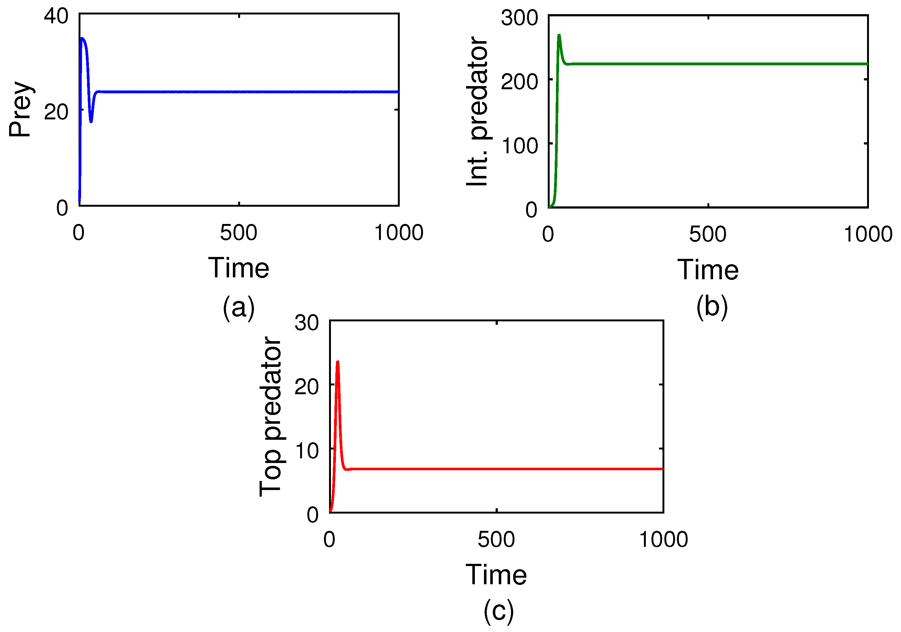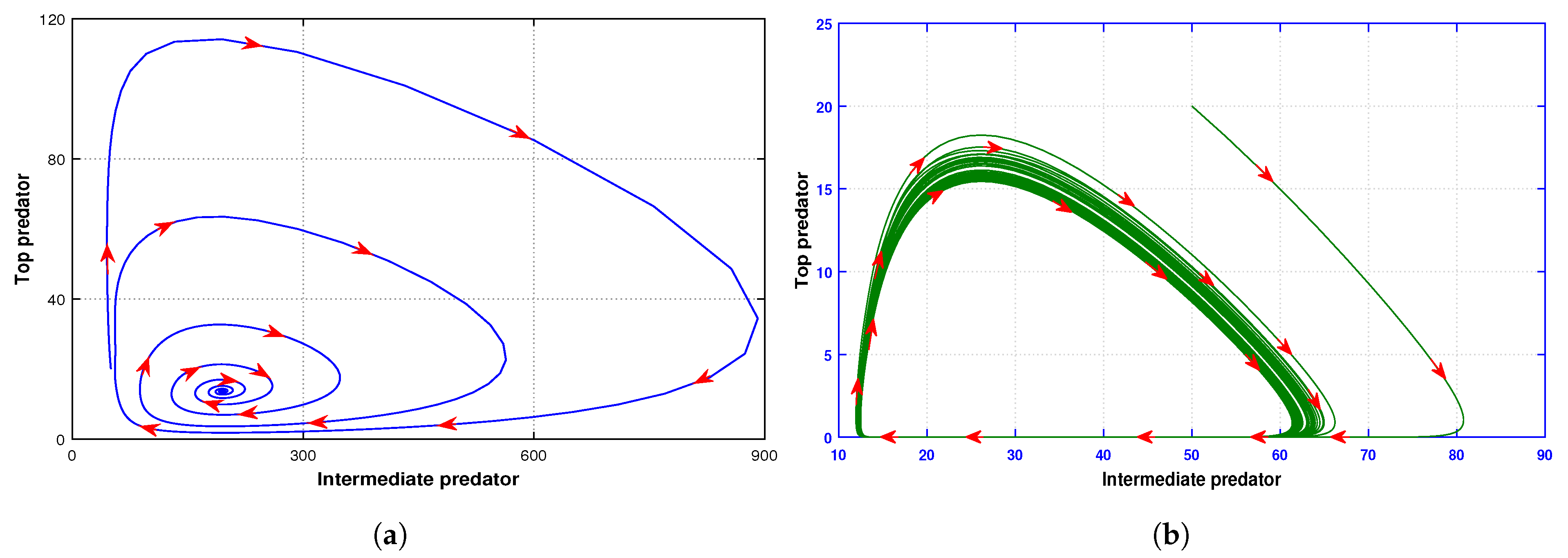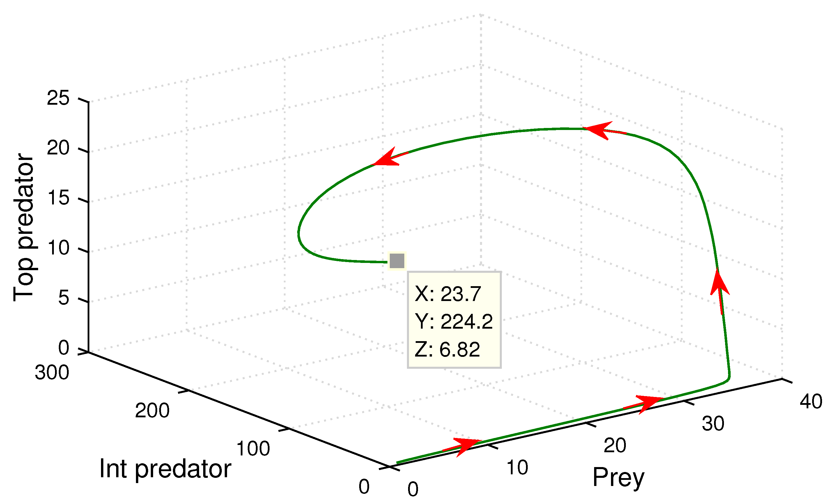Thus, we can conclude from here that the prey, intermediate predator, and top predator population coexist simultaneously (see Figure 11). Moreover, in order to analyze any dynamical behavior, a phase plane diagram is treated as one of the major tools in the non-linear system. In this connection, in Figure 12, we illustrate the phase plane nature among prey, intermediate predator, and top predator populations around the coexisting equilibrium point $E^{*}$. The figure also demonstrates the stable characteristics of the system (5).

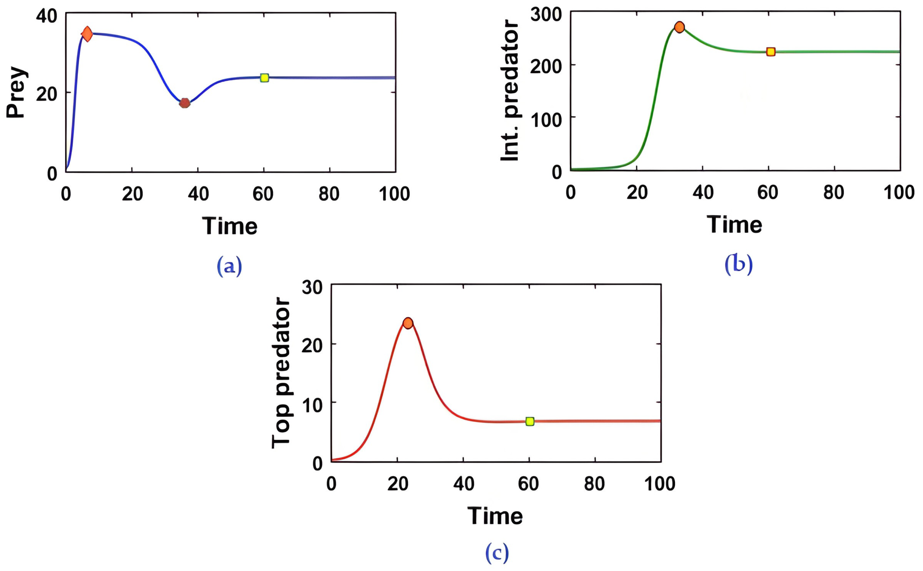
Co-existence between species is one of the essential aspects in any ecosystem. This phenomenon is well explained by Figure 3. The size profile (see Figure 3) delineates the prey population’s logistic growth with an intrinsic growth rate of $r=1.5$ and other model parameter’s magnitudes are present in the caption of that Figure 3. At the initial stage, because of the low abundance of intermediate and top predator populations, the prey population increases at a rate of $r=1.5$. But, when both the intermediate predator and top predator start to predate the prey, the predator population density begins to increase, and that of the prey population decreases rapidly. The profile Figure 3 also describes that with increasing time, i.e., $25<t<60$, the reverse-feeding mechanism takes place, i.e., the density of both the intermediate and top predators decrease simultaneously. The total feeding action is then continued between the middle and top predator, so the entire predation pressure is removed from the prey population. As a consequence, the prey species increases rapidly. Finally, all three populations achieve their steady state after a specific time $(t=60)$, and the system (5) shows stable behavior. So, it is evident that species’ co-existence is always an important issue in any ecosystem. In this regard, we propose the Theorem 6 describing the condition on which the food chains of the three species can always maintain their stability in any ecosystem.

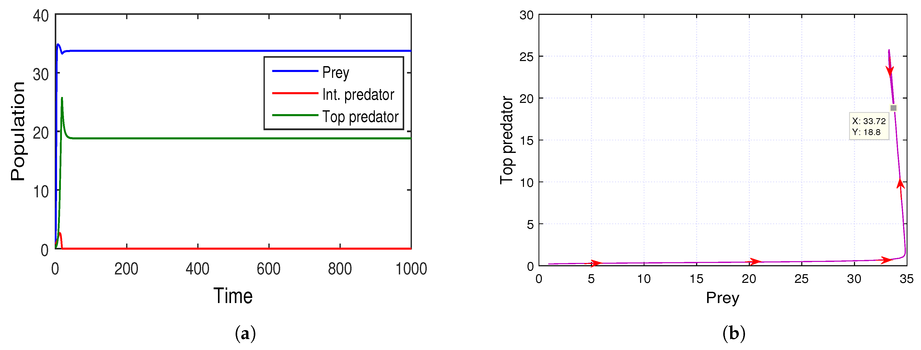
The stability of the prey-free equilibrium point $\tilde{E}(0,\tilde{N},\tilde{P})$ is also demonstrated by the Figure 13a. The figure illustrates that in the absence of the prey population, intermediate predators will face a huge amount of predation risk. The above set of parameter values provides us the prey-free equilibrium point $\tilde{E}(0,63.76,10.58)$, which is depicted in Figure 13b. We also justify the analytical conditions: (i) $r(=1.5)<\left\{\frac{{\alpha }_1\tilde{N}}{{\beta }_1}+\frac{(1-b){\alpha }_2\tilde{P}}{{\beta }_2}\right\}(=7.45)$, (ii) $tr\left(C\right)=D_1+D_4=-0.0145 (<0)$ and (iii) $det\left(C\right)=D_1{D}_4-D_2{D}_3=0.0037 (>0)$ for the stability of the system (5) at the equilibrium point $\tilde{E}$. From this observation, we determined that the predation pressure on intermediate predators by top predators should be high, as there is not enough common prey for both predators to survive. As a consequence, intermediate predators change their role from prey to predator with respect to the super-predator, i.e., the role reversal mechanism takes place in the community for the survival prospect.

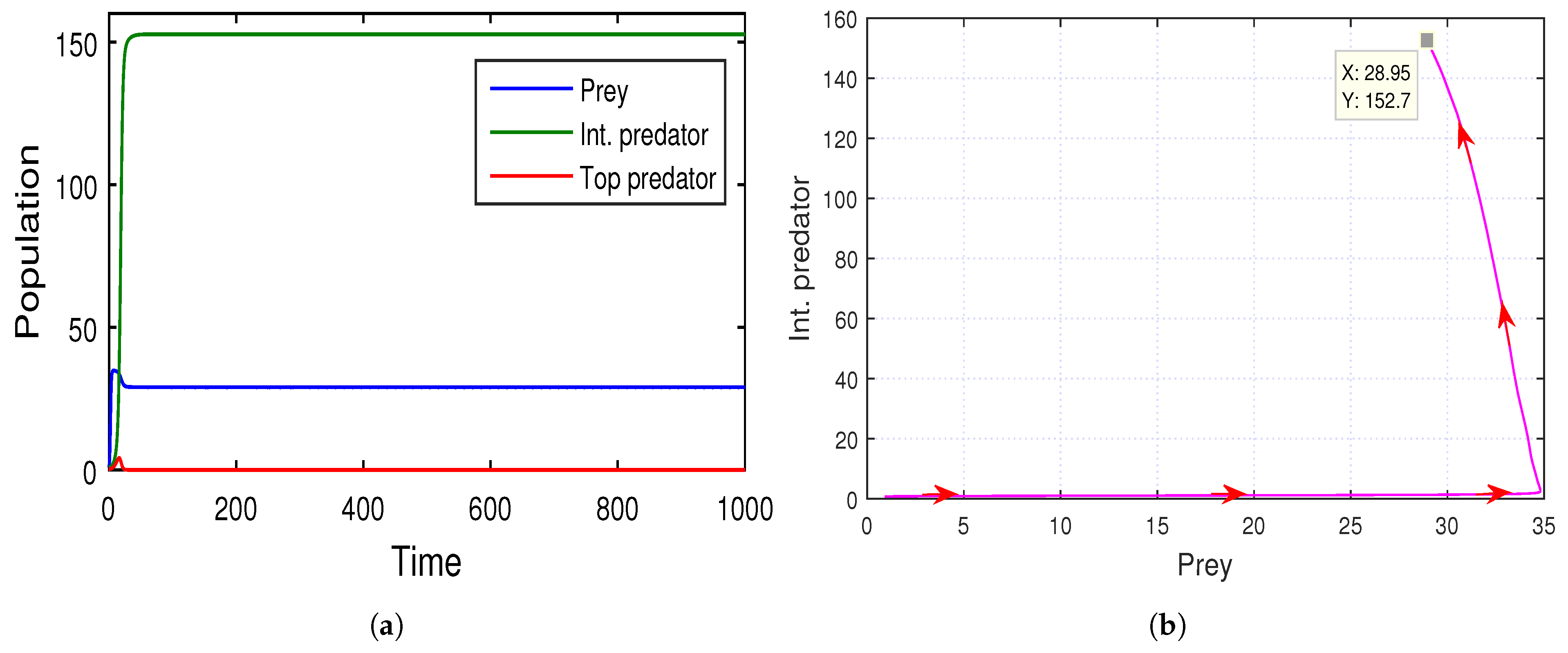
Similarly, in Figure 14, the stability of the intermediate-predator-free equilibrium point $\widehat{E}(\widehat{R},0,\widehat{P})$ is studied, where $r=1.7,$ $K=35,$ ${\alpha }_1=0.05,$ ${\beta }_1=0.6,$ ${\alpha }_2=0.25,$ ${\beta }_2=0.4,$ $e_1=0.4$, ${\alpha }_3=0.08,$ $a=0.8,$ $b=0.55,$ ${\beta }_3=0.1,$ ${\gamma }_1=0.001,$ ${\gamma }_2=0.01,$ $e_4=0.6,$ ${\alpha }_4=0.001,$ $e_2=0.5,$ $e_3=0.7,$ $d_1=0.0432,$ $d_2=0.001$, and we find that the capture rate $\left({\alpha }_2\right)$ of the immature top predator on prey and the conversion coefficient $\left(e_4\right)$ from intermediate predator to mature top predator increases. On the other hand, the value of the consumption rate $\left({\alpha }_4\right)$ of the mature intermediate predator on their immature top predator decreases, and that is why the conversion efficiency $\left(e_2\right)$ from immature top predator to mature intermediate predator also decreases due to the low rate of predation.

In Figure 15, the stability behavior of the top-predator-free equilibrium point $\overline{E}(\overline{R},\overline{N},0)$ is analyzed using the parameter set $r=1.5,$ $K=35,$ ${\alpha }_1=0.05,$ ${\beta }_1=0.6,$ ${\alpha }_2=0.18,$ ${\beta }_2=0.4,$ $e_1=0.4,$ ${\alpha }_3=0.08,$ $a=0.8,$ $b=0.25,$ ${\beta }_3=0.1,$ ${\gamma }_1=0.001,$ ${\gamma }_2=0.01,$ $e_4=0.6$, ${\alpha }_4=0.01,$ $e_2=0.5,$ $e_3=0.7,$ $d_1=0.0432,$ $d_2=0.001$, and we find that the value of consumption rates (${\alpha }_2$ and ${\alpha }_4$) of intermediate predator on prey and top predator, respectively, increase and the coefficient of intra-specific competition (${\gamma }_1$) of the intermediate predator decreases due to the availability of their food. For this reason, the axial equilibrium point $E_1(K,0,0)$ becomes unstable and the planar top predator-free equilibrium point $\overline{E}(\overline{R},\overline{N},0)$ becomes stable.

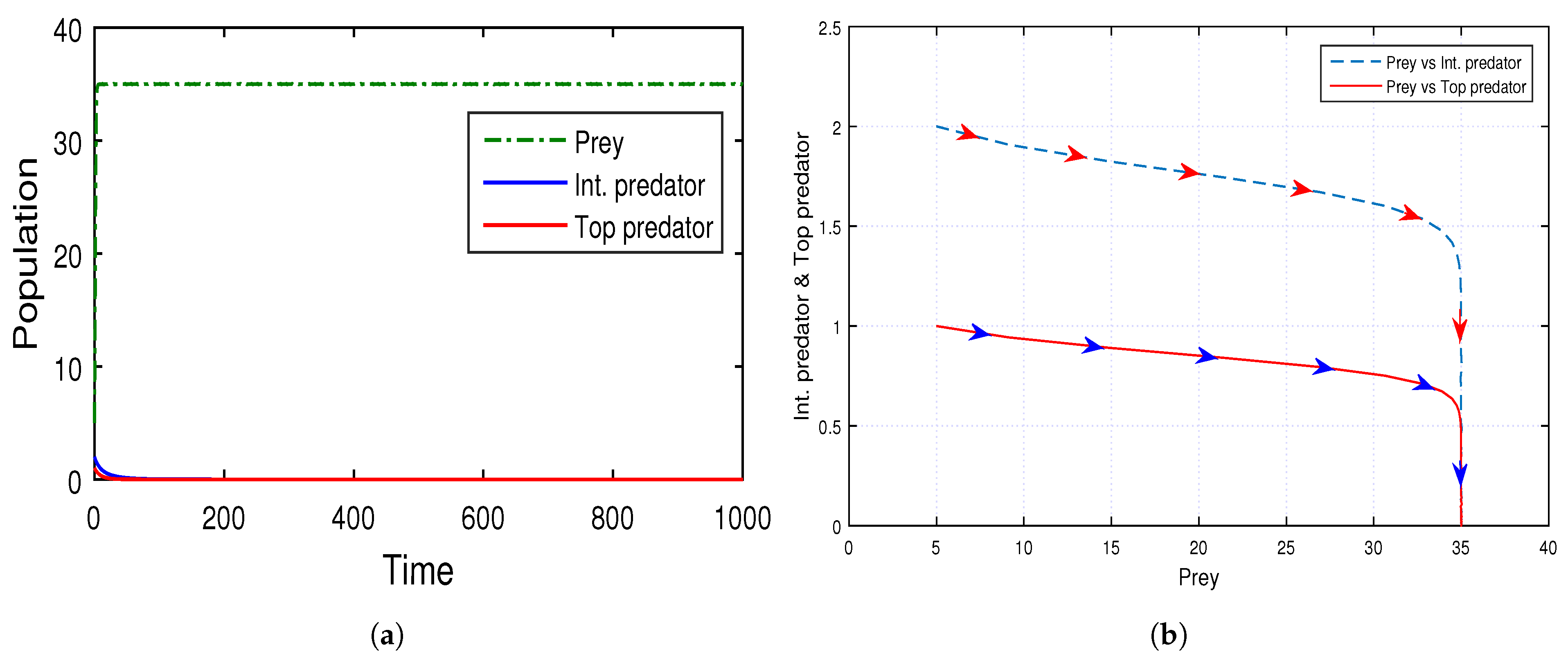
In Figure 16, we show the stability of both of the (intermediate and top) predator-free equilibrium points $E_1(K,0,0)$ by using time series with parameter values $r=1.5,$ $K=35,$ ${\alpha }_1=0.01,$ ${\beta }_1=0.6,$ ${\alpha }_2=0.01,$ ${\beta }_2=0.6,$ $e_1=0.4,$ ${\alpha }_3=0.02,$ $a=0.2,$ $b=0.15,$ ${\beta }_3=0.1,$ ${\gamma }_1=0.03,$ ${\gamma }_2=0.02,$ $e_4=0.6,$ ${\alpha }_4=0.003,$ $e_2=0.5,$ $e_3=0.7,$ $d_1=0.0432,$ $d_2=0.1$, and we find that the system (5) achieved stability at the equilibrium point $E_1$, where both intermediate and top predator populations reach extinction and the prey population reaches K (=35).

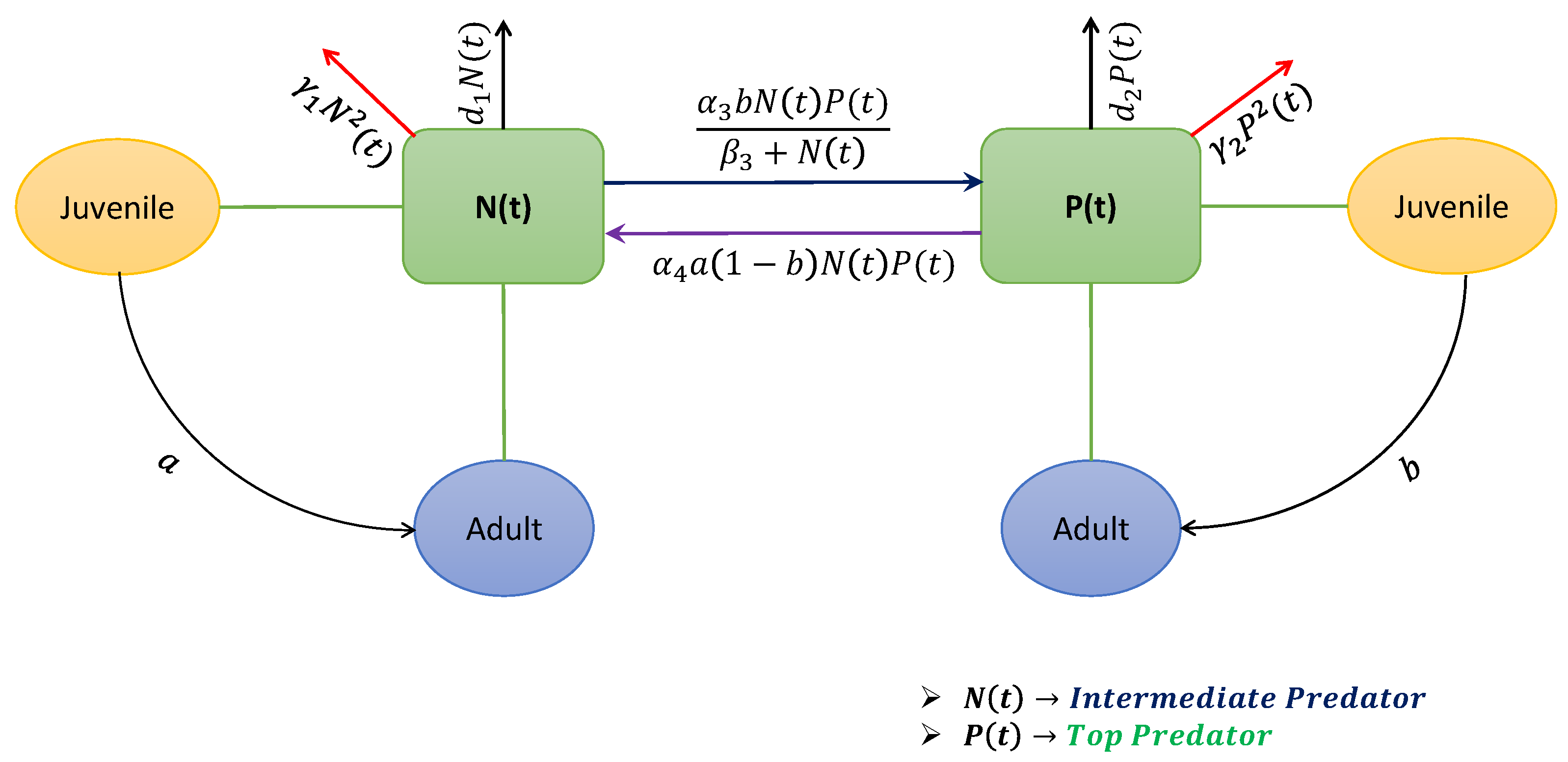
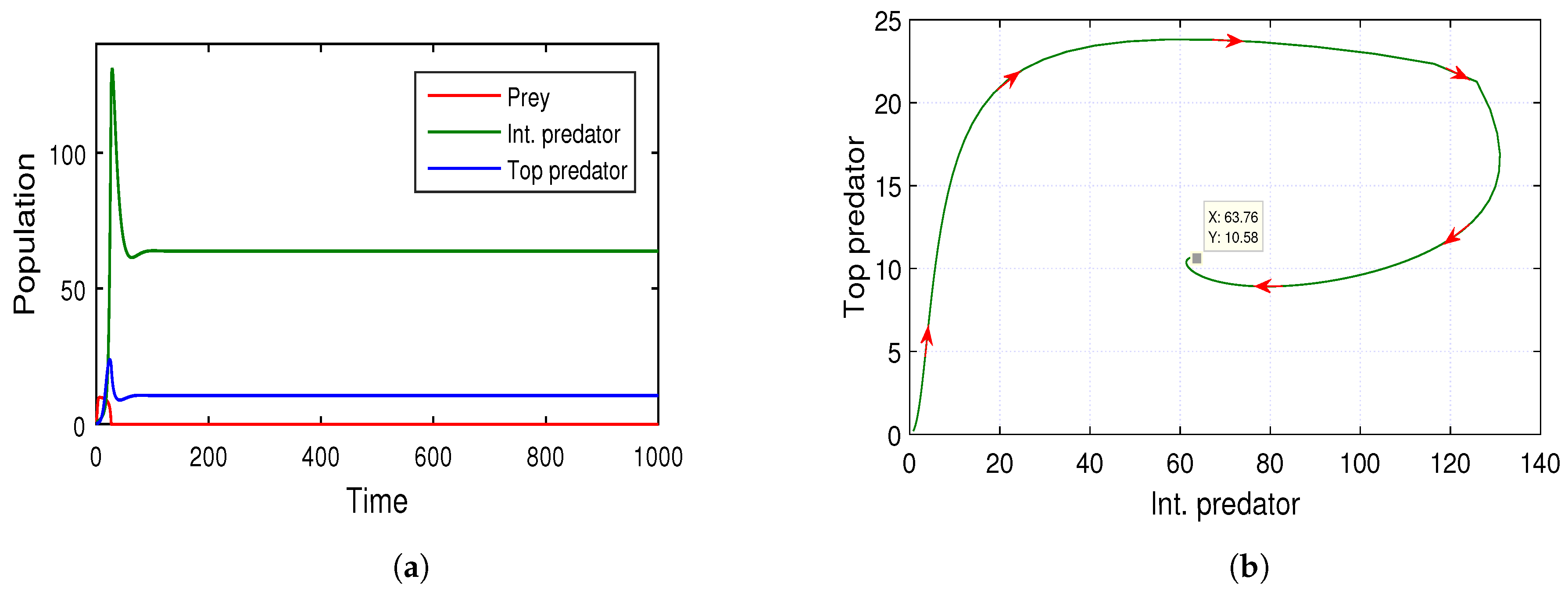
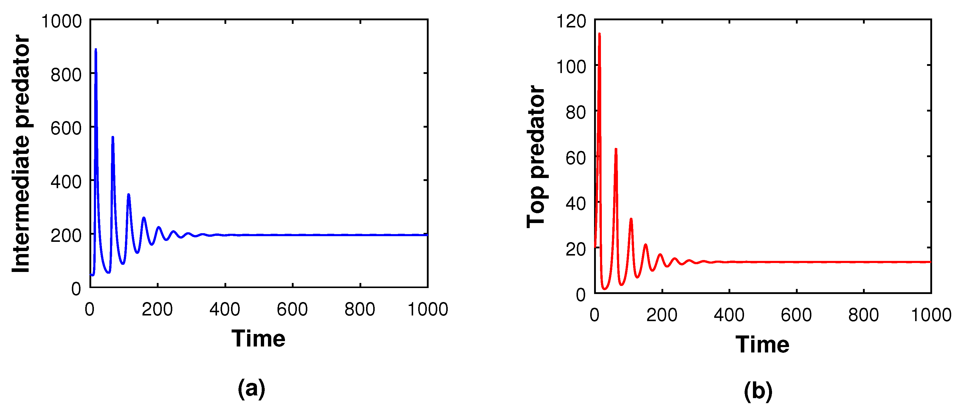
Apart from the co-existing structure, sometimes it is noticed that, in some seasons, the abundance of the prey population decreases much lower [11]. Consequently, the dynamical system of the three species is then restricted between the middle and top predators only. In this connection, we provide a necessary condition (Theorem 8) for the co-existence of the intermediate predator and the top predator in any ecosystem. This theoretical consideration is also illustrated with the numerical means in Figure 7a,b. Both of these two-dimensional figures illustrate the stability condition of the model (6). Note that the proposed condition of stability in Theorem 8 highly depends on the model parameters a, b, i.e., the transition rates from the immature to the adult stage of the intermediate and the top predator, respectively. Thus, the changing magnitudes of these transition rates will surely alter the stability of the sub-model (6). In this context, we also propose the Theorem 7 to analyze the dynamical system’s stability under the variability of the model parameters a and b. 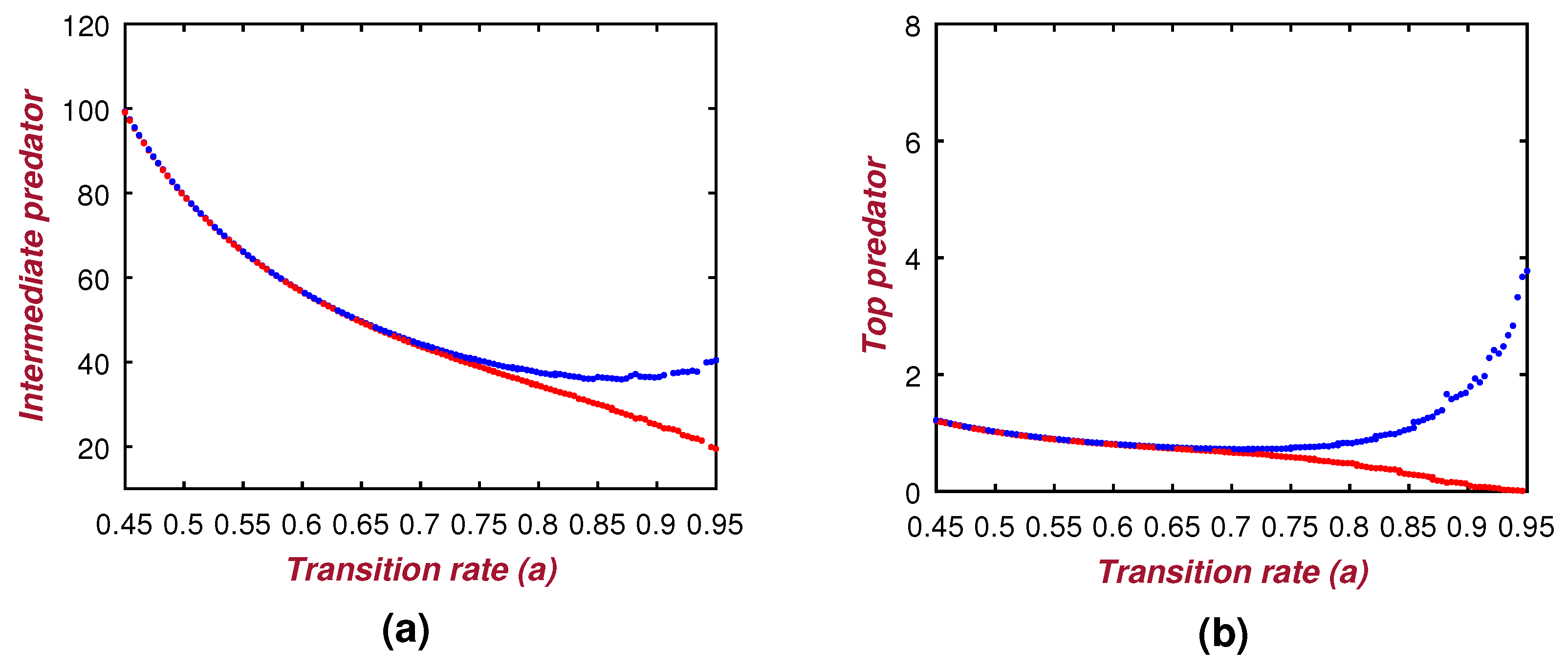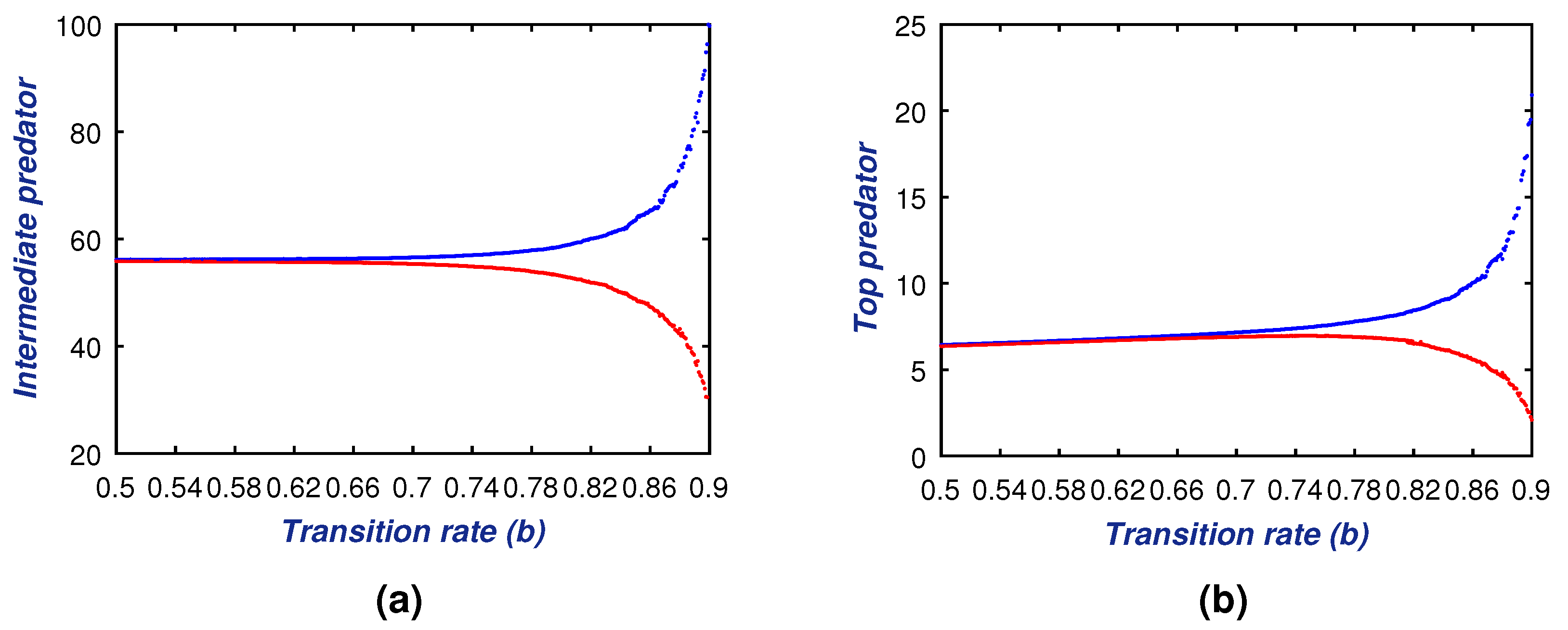The Theorem 7 with Figure 8 and Figure 9 indicate that the system (6) shows the Hopf bifurcation about the two transition rate parameters of a and b, respectively. We considered the range of these rate parameters as the semi-closed interval $[0,1)$. The bifurcation diagram (see Figure 8) indicates that the low rate of transition from the juvenile to adult stage maintains a healthy equilibrium among the intermediate and top predators. However, the high transition rates from the juvenile to adult stage enhance the effect of predation for both predatory species. As a consequence, the system (6) will show its unstable behavior. These phenomena is well explained in both of the Figure 8 and Figure 9, where it is claimed that upon exceeding the threshold values of a (i.e., 0.7) and b (i.e., 0.63), the total system becomes unstable.

Hitherto, we have discussed the deterministic scenario of the proposed tri-trophic food-web system (5). But, ecological systems are open systems, which deal with environmental influences, making any ecosystem random. Thus, it is essential to analyze the stability of any system under a stochastic environment. In this regard, we constructed the model (8) under Section 4 to discuss the stochastic nature of the tri-trophic food-web system. We followed the concept of [32] to nurture the stability in the stochastic model (8), which uses population density as the random variable. The authors elucidated that the steady state behavior of any stochastic system depends on the stability of the first three conditional central moments, i.e., the mean, variance, and skewness of the concerned random variable. 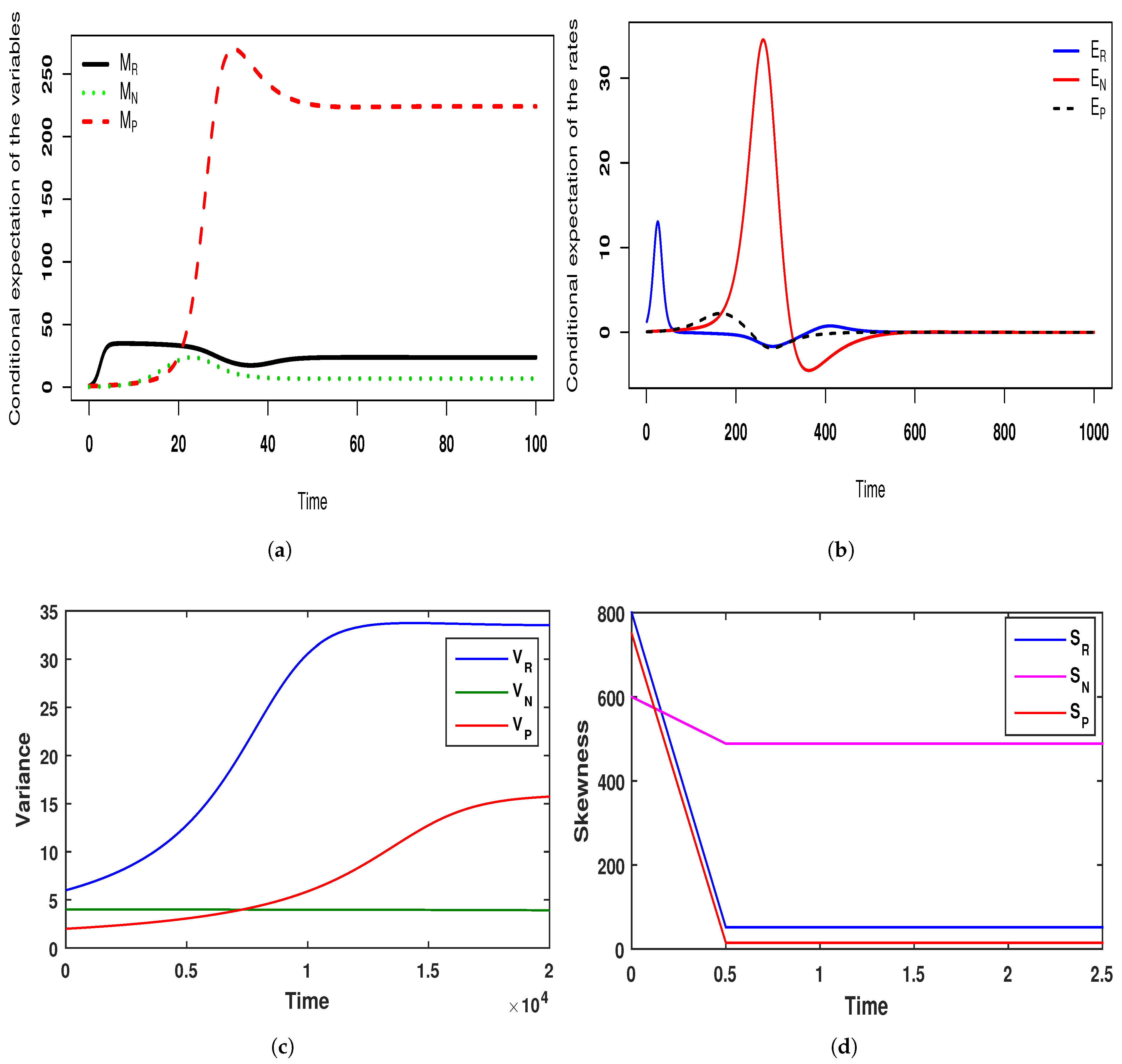To meet this objective, we established some theoretical facts for the stability of the first three conditional moments of the population random variables $R\left(t\right)$, $N\left(t\right)$, and $P\left(t\right)$, respectively. The theoretical means are also supported by the numerical scheme. 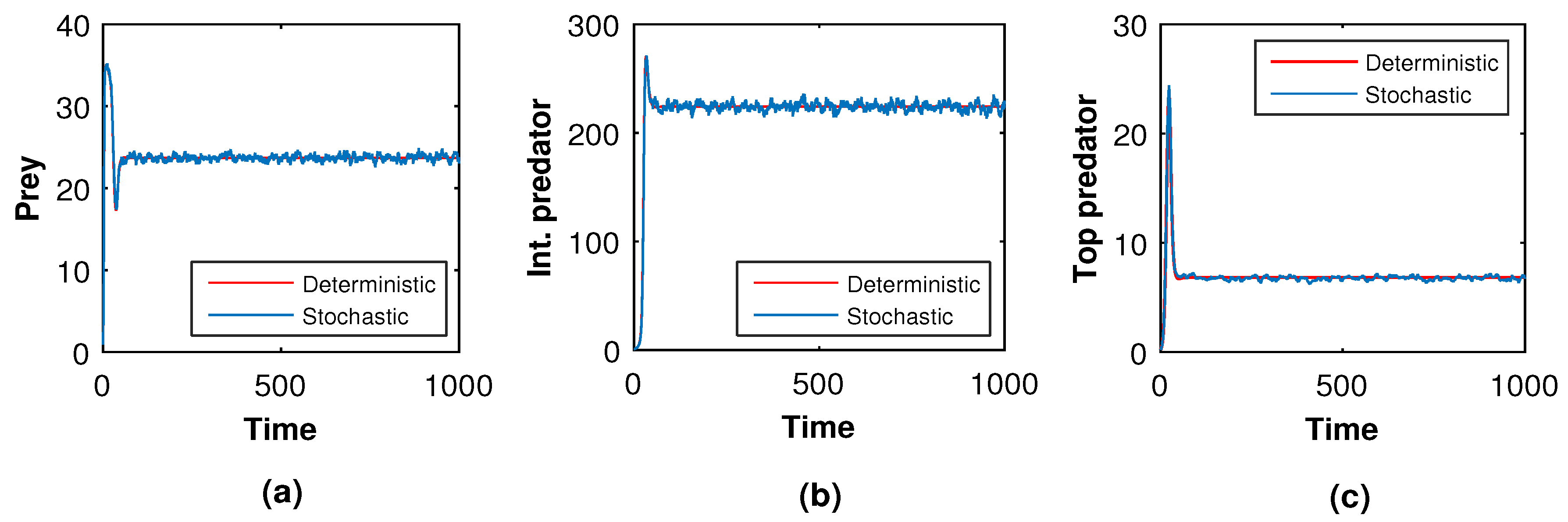In Figure 17, we see that all of the conditional moments of the species abundance converge towards their equilibrium distribution. Note that this phenomenon is justified by the time series diagram (Ref. Figure 18) and this figure shows that the solution curves of the stochastic system oscillate around the solution curves of the deterministic system. The oscillation that occurred for the stochastic system was due to the environmental noise. If the noise level is very low (Ref. Figure 19), then the solution curves for both deterministic and stochastic systems are almost identical. This clearly shows that for a certain range of parameter values, the tri-trophic food-web attains its stability in both the deterministic and stochastic case. However, we also performed a case study to observe the convergence of the equilibrium distributions for the population density as the function of control parameters. We feel that this situation can be well demonstrated by the scale parameter ${\sigma }_i(i=1,2,3)$. We considered two sets of triplet values of intensity of noise: in the first set, we considered the comparatively low intensity of noise ${\sigma }_1=0.04$, ${\sigma }_2=0.05$, and ${\sigma }_3=0.09$, and in the second set, we considered the comparatively high intensity of noise ${\sigma }_1=0.2$, ${\sigma }_2=0.3$, and ${\sigma }_3=0.5$, where the initial conditions were $R\left(0\right)=0.9,N\left(0\right)=0.8$, and $P\left(0\right)=0.2$ and the other model-associated parametric values were the same. 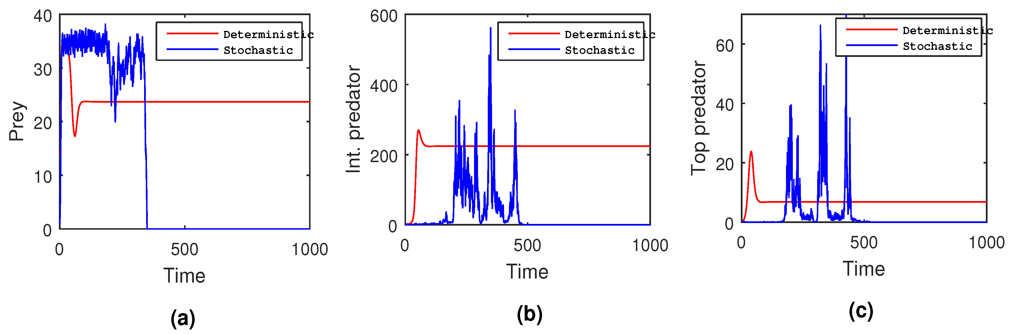The fluctuations generated in Figure 18 for the stochastic system (8) were due to the set of triplet values of intensity of noise ${\sigma }_1=0.04$, ${\sigma }_2=0.05$, and ${\sigma }_3=0.09$ and the other parametric values are mentioned in the caption of Figure 18. Taking the second set of triplet values for intensity of noise, i.e., ${\sigma }_1=0.2$, ${\sigma }_2=0.3$, and ${\sigma }_3=0.5$, with the same initial conditions and the same parametric values as for Figure 18, we created Figure 20. 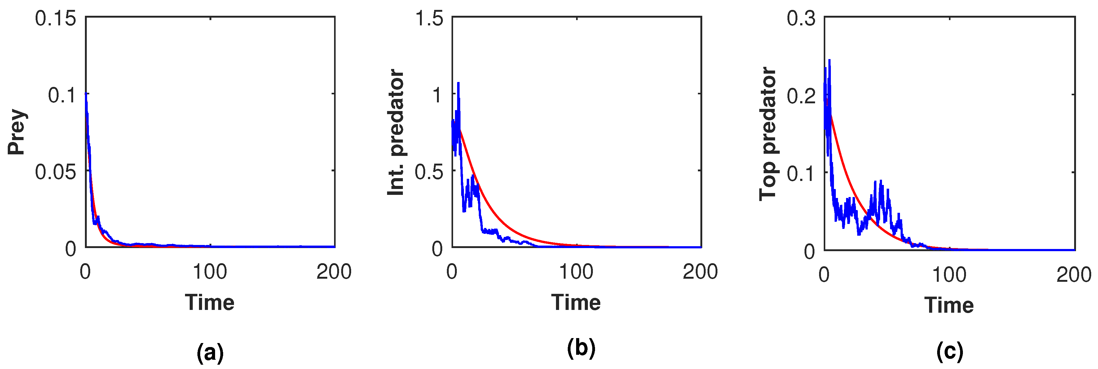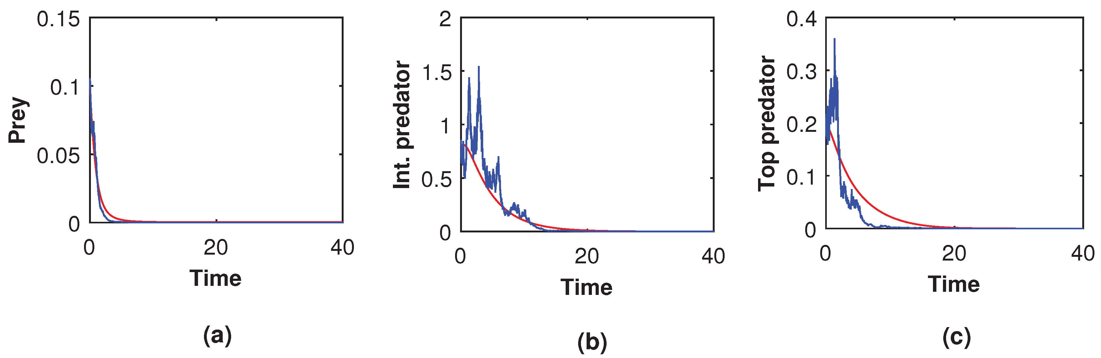From this figure (see Figure 20), it is observed that all species of the deterministic system (5) remained stable, the same as Figure 18, but all species of the stochastic system (8) disappeared completely due to the high intensity of noise. Hence, it can be concluded that various factors, such as changes in temperature, humidity, light intensity, environmental pollution, pathogens, and food quality, are responsible for the uncertain growth and deaths of interacting populations. However, these factors cannot be predetermined flawlessly. Thus, consideration of the stochastic model is more justified than the deterministic model setup.

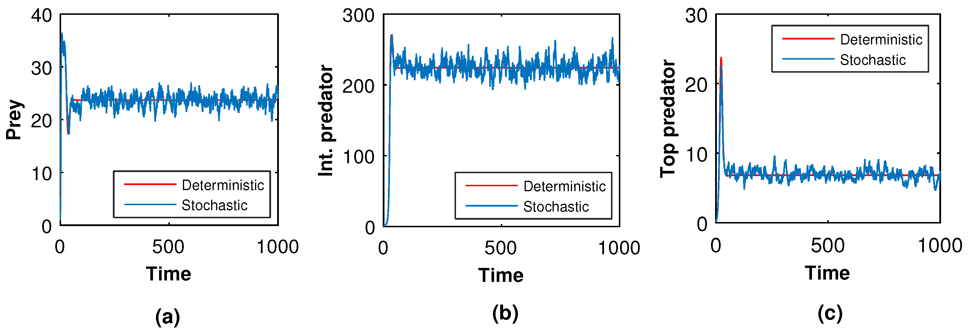
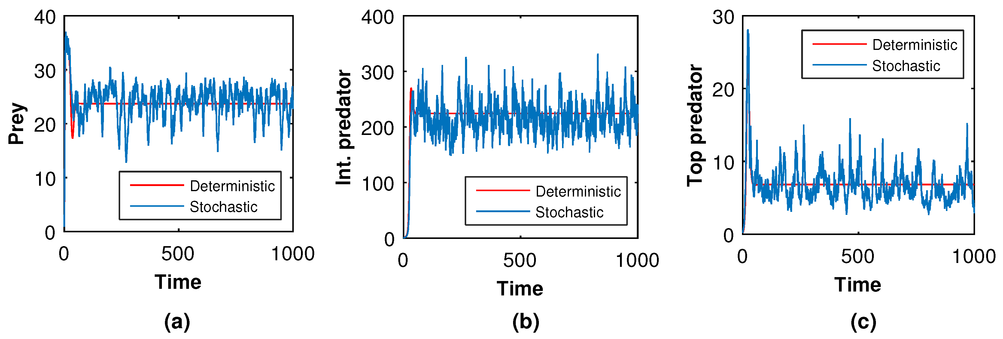
Next, we slowly raised the noise level from low to high to see what happened in the tri-trophic prey–predator interactive food chain system. Then, we showed the solution curves for both deterministic and stochastic systems for different values of the intensity of noise. In Figure 19, Figure 20, Figure 21 and Figure 22, we took the initial conditions $R\left(0\right)=0.9,$ $N\left(0\right)=0.8$, $P\left(0\right)=0.2$ and parameters $r=1.5,$ $K=35,$ ${\alpha }_1=0.2,$ ${\beta }_1=0.6,$ ${\alpha }_2=0.18,$ ${\beta }_2=0.4,$ $a=0.75,$ $b=0.5,$ $e_1=0.4,$ ${\alpha }_3=0.8,$ $e_2=0.5,$ ${\beta }_3=0.1,$ ${\gamma }_1=0.03,$ ${\gamma }_2=0.01,$ ${\alpha }_4=0.1,$ $e_3=0.7,$ $e_4=0.6,$ $d_1=0.002,$ $d_2=0.001$. The only difference among Figure 19, Figure 20, Figure 21 and Figure 22 is the intensities of environmental changes. Specially, we choose ${\sigma }_1={\sigma }_2={\sigma }_3=0.01$ in Figure 19; in Figure 21, we chose ${\sigma }_1={\sigma }_2={\sigma }_3=0.055$ and in Figure 22, we chose ${\sigma }_1={\sigma }_2={\sigma }_3=0.09$. From Figure 19, Figure 20, Figure 21 and Figure 22, we observed that the coexisting equilibrium $E^{*}(R^{*},N^{*},P^{*})$ solution curves of the stochastic model (8) always oscillated with respect to the curves of the deterministic model (5). Those figures depicted that if the intensity of the environmental changes increased, the fluctuations of the solution also increased. So, from Figure 19, Figure 20, Figure 21 and Figure 22, we arrived at the conclusion that the decrease in values of ${\sigma }_1$, ${\sigma }_2$, and ${\sigma }_3$ fluctuations fo the solution curves of the stochastic system were reduced and coincided with that of the solution curves of the deterministic system.

Under parametric values $r=0.02,$ $K=10,$ ${\alpha }_1=0.6,$ ${\beta }_1=0.6,$ ${\alpha }_2=0.8,$ ${\beta }_2=0.4,$ $a=0.75,$ $b=0.5,$ $e_1=0.4,$ ${\alpha }_3=0.8,$ $e_2=0.5,$ ${\beta }_3=0.1,$ ${\gamma }_1=0.03,$ ${\gamma }_2=0.01,$ ${\alpha }_4=0.5,$ $e_3=0.7,$ $e_4=0.6,$ $d_1=0.23,$ $d_2=0.3$ and initial conditions $R\left(0\right)=0.1,N\left(0\right)=0.7$, and $P\left(0\right)=0.1$, we created Figure 23 by taking a low intensity of noise, i.e., ${\sigma }_1=0.01$, ${\sigma }_2=0.02$, and ${\sigma }_3=0.02$, and we created Figure 24 by considering a high intensity of noise ${\sigma }_1=0.4$, ${\sigma }_2=0.3$, and ${\sigma }_3=0.8$. From both figures (Ref. Figure 23 and Figure 24), it is seen that all the species of the stochastic system (8), as well as the corresponding deterministic system (5), disappeared completely. Therefore, if the deterministic system experienced extinction, the stochastic system also experienced extinction, in which case the solution was not dependent on the intensity of the noise value (compare Figure 23 and Figure 24).

6. Conclusions

It is frequently observed that the adults of prey species sometimes show their predation mechanism on juvenile predators. Ecological literature has described this phenomenon as prey–predator role-reversal dynamics. Numerous authors have observed and explained the biological mechanism behind this feeding behavior [7,11]. However, the development of models addressing role of reversal dynamics have hardly been found in the literature, except in a few publications [20,21]. We explained the role reversal mechanism with a catastrophic change in population towards extinction through a simple prey–predator dynamic governed by two-dimensional differential equations. We believe the entire dynamics will change if an intermediate predator and stochasticity are introduced to the system. The predation mechanism of juvenile and adult members of the top and intermediate predators has a substantial impact on this reversal mechanism. Keeping these things in mind, we frame a tri-trophic food-web structure to incorporate the role-reversal dynamics. The model contains common prey with intermediate and top predators. The top predator has the ability to predate both the intermediate predator and the prey simultaneously. Because of the scarcity of the prey population and to reduce the predation risk, the intermediate predators exhibit a reverse feeding strategy towards the top predator.

A feeding mechanism due to role reversal is inevitable in ecosystems. Still, the rate at which both the intermediate and top predator populations move from being young to adults can affect how well the species can survive. The bifurcation analysis conveys that the rate of transformation rate from juvenile to adult is the key parameter for maintaining stability in this ecosystem. The transition from adolescence to adulthood creates a significant change in the characteristics of any population and achieving the subsequent reproductive qualifications of that population. The transition rate from the juvenile to adult stage of a species plays a meaningful role in predator–prey interactive dynamics. From this study, it is observed that the model system (5) transitions from a stable state to an unstable state due to the increasing value of transition rates (a and b) from juvenile to adult stage of the intermediate predator and top predator populations, respectively (Ref Figure 8 and Figure 9). The intermediate and top predator populations coexist with a stable pattern for $0.45<a<0.7$ and 2-point limit cycle oscillation for $0.7<a<0.95$. Likewise, the system shows stable coexistence of the species for $0.5<b<0.63$ and 2-point limit cycle oscillation for $0.63<b<0.9$. Therefore, a low transition rate from adolescence to adulthood maintains a healthy equilibrium among intermediate and top predators. But, the high transition rate from the juvenile to adult stage results in the model system (5) changing from a steady state to an unstable state. However, the high transition rate enhances the predation efficiency of both of the predatory species.

Moreover, we introduced stochasticity through additive noise and studied the stochastic stability of the system based on the first three-order conditional moments of the population. The convergence of the equilibrium distributions supports that under stochastic perturbation, the system (8) attains its stability. As depicted in Figure 20, the species exhibit stability in the deterministic system (5), but in the stochastic system (8), all species undergo extinction due to the exceedingly elevated noise level. Changes in light intensity, temperature, humidity, environmental pollution, pathogens, and dietary quality are, therefore, among the variables that contribute to the unpredictability of the growth and mortality of interacting populations. However, these factors cannot be perfectly predicted in a deterministic way. Therefore, the stochastic model configuration is more reasonable as a consideration in comparison with the deterministic model. To sum up, the high level of environmental noise during reversal dynamics with stochasticity causes the population to completely disappear, which is a catastrophic change compared with the deterministic counterpart.