A Finite Difference Method for Solving the Wave Equation with Fractional Damping

Abstract

In this paper, we develop a finite difference method for solving the wave equation with fractional damping in 1D and 2D cases, where the fractional damping is given based on the Caputo fractional derivative. Firstly, based on the weighted method, we propose a new numerical approximation for the Caputo fractional derivative and apply it for the 1D case to obtain a time-stepping method. We then develop an alternating direction implicit (ADI) scheme for the 2D case. Using the discrete energy method, we prove that the proposed difference schemes are unconditionally stable and convergent in both 1D and 2D cases. Finally, several numerical examples are given to verify the theoretical results.

1. Introduction

Recently, the study of damping effects has been a hot research topic because it appears in a variety of the dynamic processes of complex systems, including electromagnetic shunt [1], extensible beams [2], swelling porous elastic [3], vibration [4], and so on [5,6,7,8,9,10,11,12,13]. In this paper, we consider the initial value problem for the wave equation with fractional damping as follows:

$$\begin{array}{cc}\hfill & {\lambda }_1\frac{{\partial }^{2}u(\mathbf{x},t)}{\partial t^2}+{\lambda }_2{}_0^C{\mathcal{D}}_t^{\alpha }u(\mathbf{x},t)=D\mathsf{\Delta }u(\mathbf{x},t)+f(\mathbf{x},t),\mathbf{x}\in \mathsf{\Omega },t\in (0,T],\hfill \end{array}$$

(1)

$$\begin{array}{cc}\hfill & u(\mathbf{x},0)=\varphi \left(\mathbf{x}\right),u_t(\mathbf{x},0)=\psi \left(\mathbf{x}\right),\mathbf{x}\in \overline{\mathsf{\Omega }},\hfill \end{array}$$

(2)

$$\begin{array}{cc}\hfill & {u(\mathbf{x},t)|}_{\mathbf{x}\in \partial \mathsf{\Omega }}=\phi (\mathbf{x},t),t\in [0,T],\hfill \end{array}$$

(3)

where $\mathsf{\Omega }=(a,b)\subset {\mathbf{R}}^1$ or $\mathsf{\Omega }=(a,b)\times (c,d)\subset {\mathbf{R}}^2$, $\partial \mathsf{\Omega }$ is the boundary of $\mathsf{\Omega }$, $\mathsf{\Delta }$ is the Laplacian operator, $D(>0)$ is the diffusion coefficient, $f(\mathbf{x},t)$, $\psi (\mathbf{x},t)$, $\varphi \left(\mathbf{x}\right)$ and $\phi \left(\mathbf{x}\right)$ are given functions, and the operator ${}_0^C{\mathcal{D}}_t^{\alpha }$ denotes the Caputo fractional derivative defined by

$$\begin{array}{c}\hfill {}_0^C{\mathcal{D}}_t^{\alpha }u(\mathbf{x},t)=\frac{1}{\mathsf{\Gamma }(2-\alpha )}{\int }_0^t\frac{{\partial }^{2}u(\mathbf{x},s)}{\partial s^2}\frac{ds}{{(t-s)}^{\alpha -1}},1<\alpha <2.\end{array}$$

(4)

In an overdamped bistable system, the governing model (1)–(3) presents a double-resonance pattern [14]. The fractional derivative in Equation (1) is referred as a damping term, and can account for the memory effects in the system. The case $\alpha =\frac{3}{2}$ in Equation (1) is known as the Lokshin model, which appears in the study of the propagation of the air inside a duct when taking into account viscothermal losses [15,16]. The case $\alpha =1$ in Equation (1) is known as the damped Klein–Gordon model, arising in relativistic quantum mechanics [17]. The case $\alpha =2$ in Equation (1) is known as the classical wave equation. Compared with the above commonly discussed models, Equation (1) is more physically flexible due to the term ${}_0^C{\mathcal{D}}_t^{\alpha }u(\mathbf{x},t)$ and the parameter $\lambda$. Moreover, the inclusion of the time fractional derivative allows for the simulation of the anomalous diffusion and other non-classical transport phenomena.

Although some linear and special fractional partial differential Equations (FPDEs) can be solved using analytical methods, the analytical solutions of the most generalized FPDEs (e.g., multi-term FPDEs) cannot be worked out. Consequently, the study of efficient numerical algorithms for solving the FPDEs plays a critical role in scientific computing and engineering applications. At present, many numerical methods have been developed for solving the FPDEs, such as finite difference methods [18,19,20,21,22,23,24,25], finite element methods [26,27,28,29,30], and spectral methods [31,32].

To the best of our knowledge, only a few numerical methods for the wave equation with fractional damping in Equations (1)–(3) have been considered. Saffarian and Mohebbi [33] developed and analyzed an ADI spectral element method for solving the time fractional damped nonlinear Klein–Gordon equation, in which the equation includes the second-order derivative and the Caputo fractional derivative of order $\alpha \in (0,1)$ in the temporal direction. The WSGL scheme was used to discretize the Caputo derivative based on the relation between the Reimann–Liouville and the Caputo derivative in [33]. Wu et al. [34] used the reduced-order method to develop a Crank–Nicolson compact difference scheme of the time-fractional damped plate vibration equation, in which the equation includes the second-order derivative and the Caputo fractional derivative of order $\alpha \in (1,2)$ in the temporal direction. Based on an efficient sum-of-exponentials (SOE) approximation for the kernel function $t^{-\beta -1}$ with $\beta \in (0,1)$, Lyu et al. [35] presented a fast linearized finite difference scheme for the 1D nonlinear multi-term time-fractional wave equation, where all fractional orders are in $(1,2)$.

In this paper, we aim to propose a new finite difference method for the one- and two-dimensional wave equations with fractional damping in Equations (1)–(3). Note that a direct application of the classic $L1$ approximation to the Caputo derivative in Equation (1) at $t=t_n$ leads to a numerical scheme with only first-order temporal convergence accuracy (see [36]). The difficulty of obtaining a high-order algorithm for Equations (1)–(3) in time lies in how to design a numerical approximation with high accuracy for the following problem:

$${\lambda }_1{u}^{″}\left(t\right)+{\lambda }_2{}_0^C{\mathcal{D}}_t^{\alpha }u\left(t\right)=f\left(t\right),t\in [0,T].$$

(5)

Therefore, we first consider the difference scheme with high accuracy for Equation (5) in this study. Specifically, we consider the Caputo fractional derivative ${}_0^C{\mathcal{D}}_t^{\alpha }u\left(t\right)$ and the second-order derivative $u^{″}\left(t\right)$ as a whole in the numerical discretization, and then take its weighted average at $t=t_{n-1}$ and $t=t_{n+1}$. After careful analysis, a (3–$\alpha$)-order numerical approximation for Equation (5) is then obtained. This is one key contribution of this paper. In addition, we apply this technique of time discretization to derive numerical algorithms for the wave equation with fractional damping in Equations (1)–(3) in both 1D and 2D cases. We then use the discrete energy method to prove the unconditional stability and convergence of the proposed difference schemes. This is another novelty of our work. For the 2D case, we add some small perturbations to obtain an alternating direction implicit (ADI) scheme in order to reduce the huge computational work and storage. Finally, numerical examples are provided to verify the theoretical analysis, and to show some new diffusion-wave phenomena based on fractional damping.

2. Numerical Discretization for a Fractionally Damped System

In this section, we derive a difference scheme for solving the following fractionally damped system with initial conditions

$$\begin{array}{c}\hfill {\lambda }_1{u}^{″}\left(t\right)+{\lambda }_2{}_0^C{\mathcal{D}}_t^{\alpha }u\left(t\right)=f\left(t\right),t\in (0,T],\end{array}$$

(6)

$$\begin{array}{c}\hfill u\left(0\right)=\varphi ,u^{\prime }\left(0\right)=\psi ,\end{array}$$

(7)

where the fractional order is $\alpha \in (1,2)$, and $f\left(t\right)$ is a given source term. Here, $u^{\prime }\left(t\right)$ and $u^{″}\left(t\right)$ denote the first-order and second-order derivative with respect to t, respectively.

Take a uniform partition of the computing interval $[0,T]$, i.e., $t_n=n\tau ,0\le n\le N$ with the step size $\tau =\frac{T}{N}$, where N is a given positive integer. The numerical accuracy reaches no more than first order if we directly consider the difference scheme of Equation (6) at $t=t_n$. In order to obtain a stable difference scheme with high accuracy for Equation (6), we average the results of Equation (6) at $t=t_{n-1}$ and $t=t_{n+1}$, i.e.,

$${\lambda }_1\frac{u^{″}\left(t_{n-1}\right)+u^{″}\left(t_{n+1}\right)}{2}+{\lambda }_2\frac{{}_0^C{\mathcal{D}}_t^{\alpha }u\left(t_{n-1}\right)+{}_0^C{\mathcal{D}}_t^{\alpha }u\left(t_{n+1}\right)}{2}=\frac{f\left(t_{n-1}\right)+f\left(t_{n+1}\right)}{2}.$$

(8)

For simplicity, we define grid functions $U^n=u\left(t_n\right),n\ge 0$. Furthermore, we introduce some difference quotient operators

$${\mathsf{\Delta }}_{\tau }{U}^n=\frac{U^{n+1}-U^{n-1}}{2\tau },{\delta }_t{U}^{n-\frac{1}{2}}=\frac{U^n-U^{n-1}}{\tau },{\delta }_t^2{U}^n=\frac{{\delta }_t{U}^{n+\frac{1}{2}}-{\delta }_t{U}^{n-\frac{1}{2}}}{\tau }.$$

Firstly, we can obtain a second-order approximation for the weighted average of $u^{″}\left(t\right)$ at $t=t_{n-1}$ and $t=t_{n+1}$ by using the Taylor expansion, i.e.,

$$\frac{u^{″}\left(t_{n-1}\right)+u^{″}\left(t_{n+1}\right)}{2}={\delta }_t^2{U}^n+O\left({\tau }^2\right).$$

(9)

Next, we adopt the reduced-order method to construct our numerical formula for the Caputo derivative ${}_0^C{\mathcal{D}}_t^{\alpha }u\left(t\right)$. Let $\beta =\alpha -1,v\left(t\right)=u^{\prime }\left(t\right)$. We transform ${}_0^C{\mathcal{D}}_t^{\alpha }u\left(t\right)$ into its substitute as ${}_0^C{\mathcal{D}}_t^{\beta }v\left(t\right)$, i.e.,

$${}_0^C{\mathcal{D}}_t^{\beta }v\left(t\right)=\frac{1}{\mathsf{\Gamma }(1-\beta )}{\int }_0^t\frac{v^{\prime }\left(s\right)ds}{{(t-s)}^{\beta }}.$$

The following lemma states the truncation error of the $L1$-type fractional formula.

Lemma 1

(see [37]). Suppose $g\left(t\right)\in C^2[0,t_n]$. Then

$$\begin{array}{cc}\hfill & \left|{\int }_0^{t_n}{g}^{\prime }\left(t\right)\frac{dt}{{(t_n-t)}^{\beta }}-\frac{1}{\tau }\left[{\tilde{a}}_{0}g\left(t_n\right)-\sum _{k=1}^{n-1}({\tilde{a}}_{n-k-1}-{\tilde{a}}_{n-k})g\left(t_k\right)-{\tilde{a}}_{n-1}g\left(t_0\right)\right]\right|\hfill \\ \hfill & \le \frac{1}{1-\beta }\left[\frac{1-\beta }{12}+\frac{2^{2-\beta }}{2-\beta }-(1+2^{-\beta })\right]\underset{0\le t\le t_n}{max}\left|g^{″}\left(t\right)\right|{\tau }^{2-\beta },\hfill \end{array}$$

(10)

where $0<\beta <1$, and

$${\tilde{a}}_l={\int }_{t_l}^{t_{l+1}}\frac{dt}{t^{\beta }}=\frac{1}{1-\beta }[{\left(t_{l+1}\right)}^{1-\beta }-{\left(t_l\right)}^{1-\beta }]=\frac{{\tau }^{1-\beta }}{1-\beta }[{(l+1)}^{1-\beta }-l^{1-\beta }],l\ge 0.$$

We assume that the solution $u\left(t\right)$ of Equation (6) is smooth. Accordingly, $v\left(t\right)$ is smooth. By Lemma 1, we have the following discrete formula at grid point $t=t_n$, i.e.,

$$\begin{array}{cc}\hfill {}_0^C{\mathcal{D}}_t^{\beta }v\left(t_n\right)& =\frac{{\tau }^{-\beta }}{\mathsf{\Gamma }(2-\beta )}\left[a_0^{\left(\beta \right)}v\left(t_n\right)-\sum _{k=1}^{n-1}(a_{n-k-1}^{\left(\beta \right)}-a_{n-k}^{\left(\beta \right)})v\left(t_k\right)-a_{n-1}^{\left(\beta \right)}v\left(t_0\right)\right]+{\left(r_1\right)}^n,\hfill \end{array}$$

(11)

where $a_l^{\left(\beta \right)}={(l+1)}^{1-\beta }-l^{1-\beta },l\ge 0$, and there exists a constant $c_1$ which satisfies $|{\left(r_1\right)}^n|\le c_1{\tau }^{2-\beta }$.

Noticing the relations $\alpha =\beta +1$ and $u^{\prime }\left(t\right)=v\left(t\right)$, we then calculate the weighted average of ${}_0^C{\mathcal{D}}_t^{\alpha }u\left(t_{n+1}\right)$ and ${}_0^C{\mathcal{D}}_t^{\alpha }u\left(t_{n-1}\right)$ to yield

$$\begin{array}{cc}\hfill & \frac{{}_0^C{\mathcal{D}}_t^{\alpha }u\left(t_{n-1}\right)+{}_0^C{\mathcal{D}}_t^{\alpha }u\left(t_{n+1}\right)}{2}=\frac{{}_0^C{\mathcal{D}}_t^{\beta }v\left(t_{n-1}\right)+{}_0^C{\mathcal{D}}_t^{\beta }v\left(t_{n+1}\right)}{2}\hfill \\ \hfill & =\frac{{\tau }^{-\beta }}{\mathsf{\Gamma }(2-\beta )}[a_0^{\left(\beta \right)}\frac{v\left(t_{n-1}\right)+v\left(t_{n+1}\right)}{2}-\sum _{k=1}^{n-1}(a_{n-k-1}^{\left(\beta \right)}-a_{n-k}^{\left(\beta \right)})\frac{v\left(t_{k-1}\right)+v\left(t_{k+1}\right)}{2}\hfill \\ \hfill & -a_{n-1}^{\left(\beta \right)}\frac{v\left(t_0\right)+v\left(t_1\right)}{2}+a_n^{\left(\beta \right)}\frac{v\left(t_1\right)-v\left(t_0\right)}{2}]+\frac{{\left(r_1\right)}^{n-1}+{\left(r_1\right)}^{n+1}}{2}\hfill \\ \hfill & =\frac{{\tau }^{1-\alpha }}{\mathsf{\Gamma }(3-\alpha )}[b_0^{\left(\alpha \right)}\frac{u^{\prime }\left(t_{n-1}\right)+u^{\prime }\left(t_{n+1}\right)}{2}-\sum _{k=1}^{n-1}(b_{n-k-1}^{\left(\alpha \right)}-b_{n-k}^{\left(\alpha \right)})\frac{u^{\prime }\left(t_{k-1}\right)+u^{\prime }\left(t_{k+1}\right)}{2}\hfill \\ \hfill & -b_{n-1}^{\left(\alpha \right)}\frac{u^{\prime }\left(t_0\right)+u^{\prime }\left(t_1\right)}{2}+b_n^{\left(\alpha \right)}\frac{u^{\prime }\left(t_1\right)-u^{\prime }\left(t_0\right)}{2}]+\frac{{\left(r_1\right)}^{n-1}+{\left(r_1\right)}^{n+1}}{2},\hfill \end{array}$$

(12)

where $b_l^{\left(\alpha \right)}={(l+1)}^{2-\alpha }-l^{2-\alpha },l\ge 0$. Based on the Taylor expansion, the averaging operators in Equation (12) can be approximated using

$$\frac{1}{2}[u^{\prime }\left(t_{k-1}\right)+u^{\prime }\left(t_{k+1}\right)]={\mathsf{\Delta }}_{\tau }{U}^k+{\left(r_2\right)}^k,1\le k\le n,$$

(13)

and

$$\frac{1}{2}[u^{\prime }\left(t_k\right)+u^{\prime }\left(t_{k-1}\right)]={\delta }_t{U}^{k-\frac{1}{2}}+{\left(r_3\right)}^k,1\le k\le n,$$

(14)

where

$${\left(r_2\right)}^k=-\frac{{\tau }^2}{4}{\int }_0^1[u^{‴}(t_k-s\tau )+u^{‴}(t_k+s\tau )]{(1-s)}^{2}ds,$$

(15)

and

$${\left(r_3\right)}^k=-\frac{{\tau }^2}{16}{\int }_0^1[u^{‴}(t_{k-\frac{1}{2}}-\frac{\tau }{2}s)+u^{‴}(t_{k-\frac{1}{2}}+\frac{\tau }{2}s)]{(1-s)}^{2}ds.$$

(16)

In Equation (12), we transform $\frac{u^{\prime }\left(t_1\right)-u^{\prime }\left(t_0\right)}{2}$ into the form $\frac{u^{\prime }\left(t_1\right)+u^{\prime }\left(t_0\right)}{2}-u^{\prime }\left(t_0\right)$, and then substitute the approximations in Equations (13) and (14) into Equation (12). This gives

$$\begin{array}{cc}\hfill \frac{{}_0^C{\mathcal{D}}_t^{\alpha }u\left(t_{n-1}\right)+{}_0^C{\mathcal{D}}_t^{\alpha }u\left(t_{n+1}\right)}{2}=& \frac{{\tau }^{1-\alpha }}{\mathsf{\Gamma }(3-\alpha )}[b_0^{\left(\alpha \right)}{\mathsf{\Delta }}_{\tau }{U}^n-\sum _{k=1}^{n-1}(b_{n-k-1}^{\left(\alpha \right)}-b_{n-k}^{\left(\alpha \right)}){\mathsf{\Delta }}_{\tau }{U}^k\hfill \\ \hfill & -b_{n-1}^{\left(\alpha \right)}{\delta }_t{U}^{\frac{1}{2}}+b_n^{\left(\alpha \right)}({\delta }_t{U}^{\frac{1}{2}}-\psi )]+{\left(r_4\right)}^n,\hfill \end{array}$$

(17)

where ${\left(r_4\right)}^n$ denotes

$$\begin{array}{cc}\hfill {\left(r_4\right)}^n=& \frac{{\tau }^{1-\alpha }}{\mathsf{\Gamma }(3-\alpha )}\left[b_0^{\left(\alpha \right)}{\left(r_2\right)}^n-\sum _{k=1}^{n-1}(b_{n-k-1}^{\left(\alpha \right)}-b_{n-k}^{\left(\alpha \right)}){\left(r_2\right)}^k+(b_n^{\left(\alpha \right)}-b_{n-1}^{\left(\alpha \right)}){\left(r_3\right)}^1\right]\hfill \\ \hfill & +\frac{{\left(r_1\right)}^{n-1}+{\left(r_1\right)}^{n+1}}{2}=O\left({\tau }^{3-\alpha }\right).\hfill \end{array}$$

(18)

For simplicity, we define the operator ${\delta }_{\tau }^{\alpha }(U^n,\psi )$ as

$${\delta }_{\tau }^{\alpha }(U^n,\psi )=\frac{{\tau }^{1-\alpha }}{\mathsf{\Gamma }(3-\alpha )}\left[b_0^{\left(\alpha \right)}{\mathsf{\Delta }}_{\tau }{U}^n-\sum _{k=1}^{n-1}(b_{n-k-1}^{\left(\alpha \right)}-b_{n-k}^{\left(\alpha \right)}){\mathsf{\Delta }}_{\tau }{U}^k-b_{n-1}^{\left(\alpha \right)}{\delta }_t{U}^{\frac{1}{2}}+b_n^{\left(\alpha \right)}({\delta }_t{U}^{\frac{1}{2}}-\psi )\right].$$

(19)

Hence, based on the above numerical formulas in Equations (9) and (17), we obtain a numerical discretization for Equation (6) from the second level to the N-th level as follows:

$${\lambda }_1{\delta }_t^2{U}^n+{\lambda }_2{\delta }_{\tau }^{\alpha }(U^n,\psi )=\frac{f\left(t_{n-1}\right)+f\left(t_{n+1}\right)}{2}+R^n,1\le n\le N,$$

(20)

where $R^n=O\left({\tau }^{3-\alpha }\right)$. We now consider the numerical discretization at the first level. Since ${}_0^C{\mathcal{D}}_t^{\alpha }u\left(t_0\right)=0$, Equation (6) at $t=t_0$ reads

$${\lambda }_1{u}^{\prime \prime }\left(t_0\right)=f\left(t_0\right).$$

(21)

We apply the Taylor expansion to obtain

$$\begin{array}{c}\hfill \frac{2{\lambda }_1}{\tau }\left[{\delta }_t{U}^{\frac{1}{2}}-\psi \right]=f\left(t_0\right)+R^0,\end{array}$$

(22)

where $R^n=O\left(\tau \right)$.

Let $u^n$ be the approximate solution of $u\left(t_n\right)$. We drop the truncation error $R^n$ in Equation (20) and the truncation error $R^0$ in Equation (22) and obtain a difference scheme for Equation (6) as

$$\left\{\begin{array}{c}{\lambda }_1{\delta }_t^2{u}^n+{\lambda }_2{\delta }_{\tau }^{\alpha }(u^n,\psi )=\frac{f\left(t_{n-1}\right)+f\left(t_{n+1}\right)}{2},n\ge 1,\hfill \\ \frac{2{\lambda }_1}{\tau }\left[{\delta }_t{u}^{\frac{1}{2}}-\psi \right]=f\left(t_0\right)\hfill \end{array}\right.$$

(23)

with $u^0=\varphi$.

To verify the accuracy of the above scheme, we present an example here.

Example 1.

We take ${\lambda }_1={\lambda }_2=1$, $T=1$, $f\left(t\right)=12t^2+\frac{24}{\mathsf{\Gamma }(5-\alpha )}{t}^{4-\alpha }$ in Equation (6).

The exact solution of Example 1 is $u\left(t\right)=t^4$. In our computation, we use the difference scheme (23) to solve this problem. The numerical error was computed by

$$E_{\infty }\left(\tau \right)=\underset{0\le n\le N}{max}|u\left(t_n\right)-u^n|,$$

and the corresponding convergence order was calculated by Order $={log}_2\left(\frac{E_{\infty }\left(\tau \right)}{E_{\infty }\left(\frac{\tau }{2}\right)}\right)$.

We chose $\alpha =1.3,1.5,1.7$, respectively, to test the convergence accuracy.

Table 1. Numerical approximation error and convergence accuracy in Example 1.

$\mathit{\alpha }$	$\mathit{\tau }$	${\mathit{E}}_{\mathit{\infty }}\left(\mathit{\tau }\right)$	Order
1.3	1/2000	7.0435 × 10${}^{-7}$	-
	1/4000	2.4095 × 10${}^{-7}$	1.5476
	1/8000	8.0200 × 10${}^{-8}$	1.5871
	1/16,000	2.6193 × 10${}^{-8}$	1.6144
	1/32,000	8.4323 × 10${}^{-9}$	1.6352
	1/64,000	2.6448 × 10${}^{-9}$	1.6728
1.5	1/2000	6.4252 × 10${}^{-6}$	-
	1/4000	2.3176 × 10${}^{-6}$	1.4711
	1/8000	8.3087 × 10${}^{-7}$	1.4799
	1/16,000	2.9662 × 10${}^{-7}$	1.4860
	1/32,000	1.0558 × 10${}^{-7}$	1.4903
	1/64,000	3.7468 × 10${}^{-8}$	1.4946
1.7	1/2000	3.9280 × 10${}^{-5}$	-
	1/4000	1.6027 × 10${}^{-5}$	1.2933
	1/8000	6.5273 × 10${}^{-6}$	1.2959
	1/16,000	2.6555 × 10${}^{-6}$	1.2975
	1/32,000	1.0796 × 10${}^{-6}$	1.2985
	1/64,000	4.3871 × 10${}^{-7}$	1.2992

shows the numerical errors and the corresponding convergence accuracy for each fixed $\alpha$. As expected, our scheme (23) generates the numerical approximation accuracy with $\mathcal{O}\left({\tau }^{3-\alpha }\right)$.

3. 1D Wave Equation with Fractional Damping

In this section, we propose a finite difference method for solving Equations (1)–(3) in a one-dimensional case, i.e.,

$$\begin{array}{cc}\hfill & {\lambda }_1\frac{{\partial }^{2}u(x,t)}{\partial t^2}+{\lambda }_2{}_0^C{\mathcal{D}}_t^{\alpha }u(x,t)=D\frac{{\partial }^{2}u(x,t)}{\partial x^2}+f(x,t),x\in (a,b),t\in (0,T],\hfill \end{array}$$

(24)

$$\begin{array}{cc}\hfill & u(a,t)={\phi }_l\left(t\right),u(b,t)={\phi }_r\left(t\right),t\in (0,T],\hfill \end{array}$$

(25)

$$\begin{array}{cc}\hfill & u(x,0)=\varphi \left(x\right),\frac{\partial u(x,0)}{\partial t}=\psi \left(x\right),x\in [a,b].\hfill \end{array}$$

(26)

We then analyze the unconditional stability and convergence of the present difference method.

3.1. Derivation of the Finite Difference Method

We first consider the spatial semi-discretization for Equation (24). To this end, we design a set of the grid points as ${\mathsf{\Omega }}_h=\left\{x_i|x_i=a+ih,0\le i\le M\right\}$, where the step size $h=(b-a)/M$ and M is a positive integer. Furthermore, we define a space as

$${\mathcal{U}}_h=\{u=(u_0,u_1,\dots ,u_M)\mathrm{is}\mathrm{a}\mathrm{grid}\mathrm{function}\mathrm{on}{\mathsf{\Omega }}_h\mathrm{and}{u}_0=u_M=0\}.$$

For simplicity, we introduce some difference operators as

$${\delta }_x{u}_{i-\frac{1}{2}}=\frac{1}{h}(u_i-u_{i-1}),{\delta }_x^2{u}_i=\frac{1}{h}({\delta }_x{u}_{i+\frac{1}{2}}-{\delta }_x{u}_{i-\frac{1}{2}}),\forall u\in {\mathcal{U}}_h.$$

Suppose the solution $u(x,t)\in C_{x,t}^{(4,3)}([a,b]\times [0,T])$ of Equations (24)–(26). Here, we employ a simple second-order difference scheme for Equation (24) in spatial discretization. For simplicity, we denote $U_i\left(t\right)=u(x_i,t),0\le i\le M$. Thus, at the point $(x_i,t)$, we obtain a spatial semi-discretization scheme for Equation (24) as follows:

$${\lambda }_1\frac{{\partial }^2{U}_i\left(t\right)}{\partial t^2}+{\lambda }_2{}_0^C{\mathcal{D}}_t^{\alpha }{U}_i\left(t\right)=D{\delta }_x^2{U}_i\left(t\right)+f(x_i,t)+{\left(R_x\right)}_i\left(t\right),1\le i\le M-1,$$

(27)

where ${\left(R_x\right)}_i\left(t\right)=O\left(h^2\right)$.

Next, we apply the difference method in Equation (23) to derive the temporal discretization for Equation (24). For $n=1,\cdots ,N$, we average Equation (27) at $t=t_{n-1}$ and $t_{n+1}$ to obtain

$$\begin{array}{cc}\hfill & \frac{{\lambda }_1}{2}\left(\frac{{\partial }^2{U}_i\left(t_{n-1}\right)}{\partial t^2}+\frac{{\partial }^2{U}_i\left(t_{n+1}\right)}{\partial t^2}\right)+\frac{{\lambda }_2}{2}\left({}_0^C{\mathcal{D}}_t^{\alpha }{U}_i\left(t_{n-1}\right)+{}_0^C{\mathcal{D}}_t^{\alpha }{U}_i\left(t_{n+1}\right)\right)\hfill \\ \hfill & =\frac{D}{2}\left({\delta }_x^2{U}_i\left(t_{n-1}\right)+{\delta }_x^2{U}_i\left(t_{n+1}\right)\right)+\frac{f(x_i,t_{n-1})+f(x_i,t_{n+1})}{2}+\frac{{\left(R_x\right)}_i\left(t_{n-1}\right)+{\left(R_x\right)}_i\left(t_{n+1}\right)}{2}.\hfill \end{array}$$

(28)

For simplicity, we denote the grid points $U_i^n=u(x_i,t_n),0\le i\le M,0\le n\le N$ and introduce a symbol $U^{\overline{n}}=\frac{1}{2}(U^{n-1}+U^{n+1})$. Applying Equations (9) and (17) to Equation (28), we have

$${\lambda }_1{\delta }_t^2{U}_i^n+{\lambda }_2{\delta }_{\tau }^{\alpha }(U_i^n,{\psi }_i)=D{\delta }_x^2{U}_i^{\overline{n}}+f_i^{\overline{n}}+R_i^n,1\le i\le M-1,1\le n\le N,$$

(29)

where the truncation error $R_i^n$ satisfies

$$|R_i^n|\le c_2({\tau }^{3-\alpha }+h^2),1\le i\le M-1,1\le n\le N$$

(30)

with $c_2$ being a positive constant.

We consider Equation (27) at $t=t_0$, and then transform the result into the following equation:

$$\begin{array}{c}\hfill {\lambda }_1\frac{{\partial }^2{U}_i\left(t_0\right)}{\partial t^2}+{\lambda }_2{}_0^C{\mathcal{D}}_t^{\alpha }{U}_i\left(t_0\right)=D{\delta }_x^2{U}_i^{\frac{1}{2}}+f_i^0-\frac{D}{2}({\delta }_x^2{U}_i\left(t_1\right)-{\delta }_x^2{U}_i\left(t_0\right))+{\left(R_x\right)}_i\left(t_0\right),\end{array}$$

(31)

where $U_i^{n-\frac{1}{2}}=\frac{1}{2}(U_i^n+U_i^{n-1})$. We notice ${}_0^C{\mathcal{D}}_t^{\alpha }{U}_i\left(t_0\right)=0$ and apply the Taylor expansion to the first term in Equation (31). This gives

$$\begin{array}{c}\hfill \frac{2{\lambda }_1}{\tau }\left[{\delta }_t{U}_i^{\frac{1}{2}}-{\psi }_i\right]=D{\delta }_x^2{U}_i^{\frac{1}{2}}+f_i^0+R_i^0,\end{array}$$

(32)

where the truncation error $R_i^0$ satisfies

$$|R_i^0|\le c_3(\tau +h^2),1\le i\le M-1,$$

(33)

with $c_3$ being a positive constant.

Using the boundary conditions in Equation (25)

$$U_0^n={\phi }_l\left(t_n\right),U_M^n={\phi }_r\left(t_n\right),1\le n\le N,$$

(34)

and the initial condition in Equation (26)

$$U_i^0=\varphi \left(x_i\right),0\le i\le M,$$

(35)

dropping the small term $R_i^n$ in Equation (29) and the small term $R_i^0$ in Equation (32), and replacing $U_i^n$ with its numerical approximation $u_i^n$, we obtain a difference scheme for Equations (24)–(26) as

$$\begin{array}{cc}\hfill & {\lambda }_1{\delta }_t^2{u}_i^n+{\lambda }_2{\delta }_{\tau }^{\alpha }(u_i^n,{\psi }_i)=D{\delta }_x^2{u}_i^{\overline{n}}+f_i^{\overline{n}},1\le i\le M-1,1\le n\le N,\hfill \end{array}$$

(36)

$$\begin{array}{cc}\hfill & \frac{2{\lambda }_1}{\tau }\left[{\delta }_t{u}_i^{\frac{1}{2}}-{\psi }_i\right]=D{\delta }_x^2{u}_i^{\frac{1}{2}}+f_i^0,1\le i\le M-1,\hfill \end{array}$$

(37)

$$\begin{array}{cc}\hfill & u_0^n={\phi }_l\left(t_n\right),u_M^n={\phi }_r\left(t_n\right),1\le n\le N,\hfill \end{array}$$

(38)

$$\begin{array}{cc}\hfill & u_i^0=\varphi \left(x_i\right),0\le i\le M-1,\hfill \end{array}$$

(39)

where the truncation error is $\mathcal{O}(\tau +h^2)$ when $n=1$, and $\mathcal{O}({\tau }^{3-\alpha }+h^2)$ when $n=2,\cdots N$.

3.2. Analysis of the Difference Scheme

We now analyze the optimal error estimate of the difference scheme (36)–(39). To this end, we first define some discrete inner products and norms. For $u,v\in {\mathcal{U}}_h$, we introduce the following inner products

$$(u,v)=h\sum _{i=1}^{M-1}{u}_i{v}_i,\langle {\delta }_{x}u,{\delta }_{x}v\rangle =h\sum _{i=1}^M\left({\delta }_x{u}_{i-\frac{1}{2}}\right){\delta }_x{v}_{i-\frac{1}{2}},$$

and the corresponding norms:

$$\Vert u\Vert =\sqrt{(u,u)},{\left|u\right|}_1=\sqrt{\langle {\delta }_{x}u,{\delta }_{x}u\rangle }.$$

From the definition of ${\left\{b_n^{\left(\alpha \right)}\right\}}_{n=0}^{\infty }$ in Equation (12), we readily obtain that the properties $b_n^{\left(\alpha \right)}>0$, $b_{n-1}^{\left(\alpha \right)}>b_n^{\left(\alpha \right)},n\ge 1$. The following lemma gives an estimate of ${\delta }_{\tau }^{\alpha }({\mathsf{\Delta }}_{\tau }{v}^n,\psi )$ defined in Equation (19), which plays a crucial role in the analysis.

Lemma 1.

Let ${\delta }_{\tau }^{\alpha }({\mathsf{\Delta }}_{\tau }{v}^n,\psi )$ be defined in Equation (19). Then, we have

$$\begin{array}{cc}\hfill & \left({\delta }_{\tau }^{\alpha }({\mathsf{\Delta }}_{\tau }{v}^n,\psi )\right){\mathsf{\Delta }}_{\tau }{v}^n\hfill \\ \hfill & \ge \frac{1}{\tau }\left[\frac{{\tau }^{2-\alpha }}{2\mathsf{\Gamma }(3-\alpha )}\sum _{k=1}^n{b}_{n-k}^{\left(\alpha \right)}{\left({\mathsf{\Delta }}_{\tau }{v}^k\right)}^2-\frac{{\tau }^{2-\alpha }}{2\mathsf{\Gamma }(3-\alpha )}\sum _{k=1}^{n-1}{b}_{n-k-1}^{\left(\alpha \right)}{\left({\mathsf{\Delta }}_{\tau }{v}^k\right)}^2\right]\hfill \\ \hfill & +\frac{b_{n-1}^{\left(\alpha \right)}{\tau }^{1-\alpha }}{4\mathsf{\Gamma }(3-\alpha )}{\left({\mathsf{\Delta }}_{\tau }{v}^n\right)}^2-\frac{{\tau }^{1-\alpha }}{\mathsf{\Gamma }(3-\alpha )}\left[(b_{n-1}^{\left(\alpha \right)}-b_n^{\left(\alpha \right)}){\left({\delta }_t{v}^{\frac{1}{2}}\right)}^2+b_n^{\left(\alpha \right)}{\psi }^2\right].\hfill \end{array}$$

(40)

Proof. 

We re-write ${\delta }_{\tau }^{\alpha }({\mathsf{\Delta }}_{\tau }{v}^n,\psi )$ as the following form

$${\delta }_{\tau }^{\alpha }({\mathsf{\Delta }}_{\tau }{v}^n,\psi )=\frac{{\tau }^{1-\alpha }}{\mathsf{\Gamma }(3-\alpha )}\left[b_0^{\left(\alpha \right)}{\mathsf{\Delta }}_{\tau }{v}^n-\sum _{k=1}^{n-1}(b_{n-k-1}^{\left(\alpha \right)}-b_{n-k}^{\left(\alpha \right)}){\mathsf{\Delta }}_{\tau }{v}^k-(b_{n-1}^{\left(\alpha \right)}-b_n^{\left(\alpha \right)}){\delta }_t{v}^{\frac{1}{2}}-b_n^{\left(\alpha \right)}\psi \right].$$

(41)

Multiplying Equation (41) by ${\mathsf{\Delta }}_{\tau }{v}^n$ and using the Cauchy–Schwarz inequality, we have

$$\begin{array}{cc}\hfill ({\delta }_{\tau }^{\alpha }& ({\mathsf{\Delta }}_{\tau }{v}^n,\psi )){\mathsf{\Delta }}_{\tau }{v}^n\hfill \\ \hfill & =\frac{{\tau }^{1-\alpha }}{\mathsf{\Gamma }(3-\alpha )}[b_0^{\left(\alpha \right)}{\left({\mathsf{\Delta }}_{\tau }{v}^n\right)}^2-\sum _{k=1}^{n-1}(b_{n-k-1}^{\left(\alpha \right)}-b_{n-k}^{\left(\alpha \right)})\left({\mathsf{\Delta }}_{\tau }{v}^k\right)·{\mathsf{\Delta }}_{\tau }{v}^n\hfill \\ \hfill & -(b_{n-1}^{\left(\alpha \right)}-b_n^{\left(\alpha \right)})·\left({\delta }_t{v}^{\frac{1}{2}}\right)·{\mathsf{\Delta }}_{\tau }{v}^n-b_n^{\left(\alpha \right)}·\psi ·{\mathsf{\Delta }}_{\tau }{v}^n]\hfill \\ \hfill & \ge \frac{{\tau }^{1-\alpha }}{\mathsf{\Gamma }(3-\alpha )}[b_0^{\left(\alpha \right)}{\left({\mathsf{\Delta }}_{\tau }{v}^n\right)}^2-\sum _{k=1}^{n-1}(b_{n-k-1}^{\left(\alpha \right)}-b_{n-k}^{\left(\alpha \right)})\frac{{\left({\mathsf{\Delta }}_{\tau }{v}^k\right)}^2+{\left({\mathsf{\Delta }}_{\tau }{v}^n\right)}^2}{2}\hfill \\ \hfill & -(b_{n-1}^{\left(\alpha \right)}-b_n^{\left(\alpha \right)})\left(\frac{1}{4}{\left({\mathsf{\Delta }}_{\tau }{v}^n\right)}^2+{\left({\delta }_t{v}^{\frac{1}{2}}\right)}^2\right)-b_n^{\left(\alpha \right)}\left(\frac{1}{4}{\left({\mathsf{\Delta }}_{\tau }{v}^n\right)}^2+{\psi }^2\right)]\hfill \\ \hfill & \ge \frac{1}{\tau }\left[\frac{{\tau }^{2-\alpha }}{2\mathsf{\Gamma }(3-\alpha )}\sum _{k=1}^n{b}_{n-k}^{\left(\alpha \right)}{\left({\mathsf{\Delta }}_{\tau }{v}^k\right)}^2-\frac{{\tau }^{2-\alpha }}{2\mathsf{\Gamma }(3-\alpha )}\sum _{k=1}^{n-1}{b}_{n-k-1}^{\left(\alpha \right)}{\left({\mathsf{\Delta }}_{\tau }{v}^k\right)}^2\right]\hfill \\ \hfill & +\frac{b_{n-1}^{\left(\alpha \right)}{\tau }^{1-\alpha }}{4\mathsf{\Gamma }(3-\alpha )}{\left({\mathsf{\Delta }}_{\tau }{v}^n\right)}^2-\frac{{\tau }^{1-\alpha }}{\mathsf{\Gamma }(3-\alpha )}\left[(b_{n-1}^{\left(\alpha \right)}-b_n^{\left(\alpha \right)}){\left({\delta }_t{v}^{\frac{1}{2}}\right)}^2+b_n^{\left(\alpha \right)}{\psi }^2\right].\hfill \end{array}$$

(42)

Hence, we have completed the proof. □

We now derive a prior estimate of the scheme (36)–(39).

Lemma 2.

Suppose that $\left\{v_i^n\right\}$ is the solution of the scheme

$$\begin{array}{cc}\hfill & {\lambda }_1{\delta }_t^2{v}_i^n+{\lambda }_2{\delta }_{\tau }^{\alpha }(v_i^n,{\tilde{\psi }}_i)=D{\delta }_x^2{v}_i^{\overline{n}}+g_i^{\overline{n}},1\le i\le M-1,1\le n\le N,\hfill \end{array}$$

(43)

$$\begin{array}{cc}\hfill & \frac{2{\lambda }_1}{\tau }\left[{\delta }_t{v}_i^{\frac{1}{2}}-{\tilde{\psi }}_i\right]=D{\delta }_x^2{v}_i^{\frac{1}{2}}+g_i^0,1\le i\le M-1,\hfill \end{array}$$

(44)

$$\begin{array}{cc}\hfill & v_0^n=0,v_M^n=0,1\le n\le N,\hfill \end{array}$$

(45)

$$\begin{array}{cc}\hfill & v_i^0={\tilde{\varphi }}_i,0\le i\le M-1.\hfill \end{array}$$

(46)

Then, it holds that

$$|v^n{|}_1^2\le C(D,{\lambda }_1,{\lambda }_2,T,\alpha )\left(\right|v^0{|}_1^2+\parallel \tilde{\psi }{\parallel }^2+{\tau }^2\parallel g^0{\parallel }^2+\tau \sum _{m=1}^n\parallel g^{\overline{m}}{\parallel }^2).$$

(47)

Proof. 

We take an inner product of Equation (44) with ${\delta }_t{v}^{\frac{1}{2}}$ to obtain

$$\frac{2{\lambda }_1}{\tau }({\delta }_t{v}^{\frac{1}{2}}-\tilde{\psi },{\delta }_t{v}^{\frac{1}{2}})=D({\delta }_x^2{v}^{\frac{1}{2}},{\delta }_t{v}^{\frac{1}{2}})+(g^0,{\delta }_t{v}^{\frac{1}{2}}).$$

(48)

Multiplying both sides of Equation (48) by $\tau$, we obtain

$$2{\lambda }_1{\parallel {\delta }_t{v}^{\frac{1}{2}}\parallel }^2=D\tau ({\delta }_x^2{v}^{\frac{1}{2}},{\delta }_t{v}^{\frac{1}{2}})+2{\lambda }_1(\tilde{\psi },{\delta }_t{v}^{\frac{1}{2}})+\tau (g^0,{\delta }_t{v}^{\frac{1}{2}}).$$

(49)

Applying the summation by parts to the first term on the right-hand side of Equation (49) leads to

$$D\tau ({\delta }_x^2{v}^{\frac{1}{2}},{\delta }_t{v}^{\frac{1}{2}})=-\frac{D}{2}(|v^1{|}_1^2+|v^0{|}_1^2)+D|v^0{|}_1^2.$$

(50)

Using the Cauchy–Schwarz inequality to the last two terms on the right-hand side of Equation (49) gives

$$2{\lambda }_1(\tilde{\psi },{\delta }_t{v}^{\frac{1}{2}})\le \frac{{\lambda }_1}{2}\parallel {\delta }_t{v}^{\frac{1}{2}}{\parallel }^2+2{\lambda }_1{\parallel \tilde{\psi }\parallel }^2,$$

(51)

and

$$\tau (g^0,{\delta }_t{v}^{\frac{1}{2}})\le \frac{{\lambda }_1}{2}\parallel {\delta }_t{v}^{\frac{1}{2}}{\parallel }^2+\frac{{\tau }^2}{2{\lambda }_1}{\parallel g^0\parallel }^2.$$

(52)

Inserting Equations (50)–(52) into Equation (49) leads to

$${\lambda }_1\parallel {\delta }_t{v}^{\frac{1}{2}}{\parallel }^2+\frac{D}{2}\left(\right|v^1{|}_1^2+|v^0{|}_1^2)\le D|v^0{|}_1^2+2{\lambda }_1\parallel \tilde{\psi }{\parallel }^2+\frac{{\tau }^2}{2{\lambda }_1}{\parallel g^0\parallel }^2.$$

(53)

We take an inner product of Equation (43) with ${\mathsf{\Delta }}_{\tau }{v}^n$ as

$${\lambda }_1({\delta }_t^2{v}^n,{\mathsf{\Delta }}_{\tau }{v}^n)+{\lambda }_2({\delta }_{\tau }^{\alpha }(v^n,\tilde{\psi }),{\mathsf{\Delta }}_{\tau }{v}^n)=D({\delta }_x^2{v}^{\overline{n}},{\mathsf{\Delta }}_{\tau }{v}^n)+(g^{\overline{n}},{\mathsf{\Delta }}_{\tau }{v}^n).$$

(54)

After careful analysis, we obtain

$${\lambda }_1({\delta }_t^2{v}^n,{\mathsf{\Delta }}_{\tau }{v}^n)=\frac{{\lambda }_1}{2\tau }\left(\Vert {\delta }_t{v}^{n+\frac{1}{2}}{\Vert }^2-{\Vert {\delta }_t{v}^{n-\frac{1}{2}}\Vert }^2\right).$$

(55)

Applying the summation by parts to the first term on the right-hand side of Equation (54) and noticing the boundary conditions in Equation (45), we have

$$D({\delta }_x^2{v}^{\overline{n}},{\mathsf{\Delta }}_{\tau }{v}^n)=-\frac{D}{4\tau }\left(\right|v^{n+1}{|}_1^2-|v^{n-1}{|}_1^2).$$

(56)

We denote $E^n=\frac{{\lambda }_2{\tau }^{2-\alpha }}{2\mathsf{\Gamma }(3-\alpha )}{\displaystyle \sum _{k=1}^n}{b}_{n-k}^{\left(\alpha \right)}{\parallel {\mathsf{\Delta }}_{\tau }{v}^k\parallel }^2$. By Lemma 1, we obtain

$$\begin{array}{cc}\hfill {\lambda }_2({\delta }_{\tau }^{\alpha }(v^n,\tilde{\psi }),{\mathsf{\Delta }}_{\tau }{v}^n)\ge & \frac{1}{\tau }(E^n-E^{n-1})+\frac{{\lambda }_2{b}_{n-1}^{\left(\alpha \right)}{\tau }^{1-\alpha }}{4\mathsf{\Gamma }(3-\alpha )}{\parallel {\mathsf{\Delta }}_{\tau }{v}^n\parallel }^2\hfill \\ \hfill & -\frac{{\lambda }_2{\tau }^{1-\alpha }}{\mathsf{\Gamma }(3-\alpha )}\left[(b_{n-1}^{\left(\alpha \right)}-b_n^{\left(\alpha \right)})\parallel {\delta }_t{v}^{\frac{1}{2}}{\parallel }^2+b_n^{\left(\alpha \right)}{\parallel \tilde{\psi }\parallel }^2\right].\hfill \end{array}$$

(57)

We further apply the Cauchy–Schwarz inequality to the last term on the right-hand side of Equation (54). This gives

$$(g^{\overline{n}},{\mathsf{\Delta }}_{\tau }{v}^n)\le \frac{{\lambda }_2{b}_{n-1}^{\left(\alpha \right)}{\tau }^{1-\alpha }}{4\mathsf{\Gamma }(3-\alpha )}\parallel {\mathsf{\Delta }}_{\tau }{v}^n{\parallel }^2+\frac{\mathsf{\Gamma }(2-\alpha )t_n^{\alpha -1}}{{\lambda }_2}{\parallel \overline{g}\parallel }^2.$$

(58)

For simplicity, we denote $F^n=E^n+\frac{{\lambda }_1}{2}\parallel {\delta }_t{v}^{n+\frac{1}{2}}{\parallel }^2+\frac{D}{4}\left(\right|v^{n+1}{|}_1^2+|v^n{|}_1^2)$. Substituting Equations (55)–(58) into Equation (54) leads to

$$\begin{array}{c}\hfill \frac{1}{\tau }(F^n-F^{n-1})\le \frac{{\lambda }_2{\tau }^{1-\alpha }}{\mathsf{\Gamma }(3-\alpha )}\left[(b_{n-1}^{\left(\alpha \right)}-b_n^{\left(\alpha \right)})\parallel {\delta }_t{v}^{\frac{1}{2}}{\parallel }^2+b_n^{\left(\alpha \right)}{\parallel \tilde{\psi }\parallel }^2\right]+\frac{\mathsf{\Gamma }(2-\alpha )t_n^{\alpha -1}}{{\lambda }_2}{\parallel g^{\overline{n}}\parallel }^2.\end{array}$$

(59)

Multiplying Equation (59) by $\tau$, we obtain

$$F^n\le F^{n-1}+\frac{{\lambda }_2{\tau }^{2-\alpha }}{\mathsf{\Gamma }(3-\alpha )}\left[(b_{n-1}^{\left(\alpha \right)}-b_n^{\left(\alpha \right)})\parallel {\delta }_t{v}^{\frac{1}{2}}{\parallel }^2+b_n^{\left(\alpha \right)}{\parallel \tilde{\psi }\parallel }^2\right]+\frac{\mathsf{\Gamma }(2-\alpha )t_n^{\alpha -1}}{{\lambda }_2}\tau {\parallel g^{\overline{n}}\parallel }^2.$$

(60)

Replacing n with m in Equation (60) and then summing up for m from 1 to n on both sides of the result, we have

$$\begin{array}{cc}\hfill F^n\le & F^0+\frac{{\lambda }_2{\tau }^{2-\alpha }}{\mathsf{\Gamma }(3-\alpha )}\left[\sum _{m=1}^n(b_{m-1}^{\left(\alpha \right)}-b_m^{\left(\alpha \right)})\parallel {\delta }_t{v}^{\frac{1}{2}}{\parallel }^2+\sum _{m=1}^n{b}_m^{\left(\alpha \right)}{\parallel \tilde{\psi }\parallel }^2\right]\hfill \\ \hfill & +\frac{\mathsf{\Gamma }(2-\alpha )}{{\lambda }_2}\tau \sum _{m=1}^n{t}_m^{\alpha -1}{\parallel g^{\overline{m}}\parallel }^2.\hfill \end{array}$$

(61)

Using the following relations

$$\sum _{m=1}^n(b_{m-1}^{\left(\alpha \right)}-b_m^{\left(\alpha \right)})=b_0^{\left(\alpha \right)}-b_n^{\left(\alpha \right)}<b_0^{\left(\alpha \right)}=1,$$

(62)

$$\sum _{m=1}^n{b}_m^{\left(\alpha \right)}=\sum _{m=1}^n[{(m+1)}^{2-\alpha }-m^{2-\alpha }]={(n+1)}^{2-\alpha }-1<{(n+1)}^{2-\alpha },$$

(63)

and $t_m^{\alpha -1}\le t_n^{\alpha -1}$, $m=1,2,\cdots ,n$ for Equation (61), we obtain

$$F^n\le F^0+\frac{{\lambda }_2{\tau }^{2-\alpha }}{\mathsf{\Gamma }(3-\alpha )}\parallel {\delta }_t{v}^{\frac{1}{2}}{\parallel }^2+\frac{{\lambda }_2{t}_{n+1}^{2-\alpha }}{\mathsf{\Gamma }(3-\alpha )}\parallel \tilde{\psi }{\parallel }^2+\frac{\mathsf{\Gamma }(2-\alpha )t_n^{\alpha -1}}{{\lambda }_2}\tau \sum _{m=1}^n{\parallel g^{\overline{m}}\parallel }^2.$$

(64)

Applying Equation (53) to estimate $F^0$ and $\parallel {\delta }_t{v}^{\frac{1}{2}}{\parallel }^2$, we have

$$\begin{array}{cc}\hfill F^n\le & \left(\frac{D}{2}+\frac{{\lambda }_{2}D{\tau }^{2-\alpha }}{{\lambda }_1\mathsf{\Gamma }(3-\alpha )}\right)|v^0{|}_1^2+\left({\lambda }_1+\frac{2{\lambda }_2{\tau }^{2-\alpha }}{\mathsf{\Gamma }(3-\alpha )}+\frac{{\lambda }_2{t}_{n+1}^{2-\alpha }}{\mathsf{\Gamma }(3-\alpha )}\right){\parallel \tilde{\psi }\parallel }^2\hfill \\ \hfill & +\frac{{\lambda }_2{\tau }^{4-\alpha }}{2{\lambda }_1^2\mathsf{\Gamma }(3-\alpha )}\parallel g^0{\parallel }^2+\frac{\mathsf{\Gamma }(2-\alpha )t_n^{\alpha -1}}{{\lambda }_2}\tau \sum _{m=1}^n{\parallel g^{\overline{m}}\parallel }^2.\hfill \end{array}$$

(65)

Hence, we have completed the proof. □

Based on Lemma 2, we have the following theorem for stability of the scheme (36)–(39).

Theorem 3

(Stability). Assume that $\left\{{\left(u^1\right)}_i^n\right\}$ and $\left\{{\left(u^2\right)}_i^n\right\}$ are two numerical solutions obtained based on the scheme (36)–(39) with same initial and boundary conditions but different source terms ${\left(f^{\left(1\right)}\right)}_i^n$ and ${\left(f^{\left(2\right)}\right)}_i^n$. Let $u_i^n={\left(u^{\left(1\right)}\right)}_i^n-{\left(u^{\left(2\right)}\right)}_i^n$ and $f_i^n={\left(f^{\left(1\right)}\right)}_i^n-{\left(f^{\left(2\right)}\right)}_i^n$. Then, it holds that

$$\parallel u^n{\parallel }_{\infty }^2\le C(D,{\lambda }_1,{\lambda }_2,T,\alpha )({\tau }^2\parallel f^0{\parallel }^2+\tau \sum _{m=1}^n\parallel f^{\overline{m}}{\parallel }^2).$$

(66)

This implies that the scheme (36)–(39) is unconditionally stable.

We now give the error estimate of the difference scheme (36)–(39). Let $e_i^n=U_i^n-u_i^n,0\le i\le M,0\le n\le N$. Subtracting Equations (36)–(39) from Equations (29), (32), (34) and (35), we obtain error equations as follows:

$$\begin{array}{cc}\hfill & {\lambda }_1{\delta }_t^2{e}_i^n+{\lambda }_2{\delta }_{\tau }^{\alpha }(e_i^n,0)=D{\delta }_x^2{e}_i^{\overline{n}}+R_i^n,1\le i\le M-1,1\le n\le N,\hfill \end{array}$$

(67)

$$\begin{array}{cc}\hfill & \frac{2{\lambda }_1}{\tau }{\delta }_t{e}_i^{\frac{1}{2}}=D{\delta }_x^2{e}_i^{\frac{1}{2}}+R_i^0,1\le i\le M-1,\hfill \end{array}$$

(68)

$$\begin{array}{cc}\hfill & e_0^n=0,e_M^n=0,1\le n\le N,\hfill \end{array}$$

(69)

$$\begin{array}{cc}\hfill & e_i^0=0,0\le i\le M-1.\hfill \end{array}$$

(70)

Theorem 4

(Convergence). Suppose that the solution $u(x,t)\in C_{x,t}^{(4,3)}([a,b]\times [0,T])$ of 1D wave equation with fractional damping (24)–(26), and $\left\{u_i^n\right|0\le i\le M,0\le n\le N\}$ is the solution of the difference scheme (36)–(39). Then, the following optimal error estimate holds

$$\parallel U^n-u^n{\parallel }_{\infty }\le C({\tau }^{3-\alpha }+h^2),1\le n\le N,$$

(71)

which implies that the numerical solution is convergent to the analytical solution with the error $O({\tau }^{3-\alpha }+h^2)$.

Proof. 

We take an inner product of Equation (68) with ${\delta }_t{e}^{\frac{1}{2}}$ and Equation (67) with ${\mathsf{\Delta }}_{\tau }{e}^n$, respectively. This gives

$$\frac{2{\lambda }_1}{\tau }({\delta }_t{e}^{\frac{1}{2}},{\delta }_t{e}^{\frac{1}{2}})=D({\delta }_x^2{e}^{\frac{1}{2}},{\delta }_t{e}^{\frac{1}{2}})+(R^0,{\delta }_t{e}^{\frac{1}{2}}),$$

(72)

and

$${\lambda }_1({\delta }_t^2{e}^n,{\mathsf{\Delta }}_{\tau }{e}^n)+{\lambda }_2({\delta }_{\tau }^{\alpha }(e^n,0),{\mathsf{\Delta }}_{\tau }{e}^n)=D({\delta }_x^2{e}^{\overline{n}},{\mathsf{\Delta }}_{\tau }{e}^n)+(R^n,{\mathsf{\Delta }}_{\tau }{e}^n).$$

(73)

Adopting the analysis strategy in Lemma 2, we have

$$\parallel e^n{\parallel }_{\infty }^2\le C(D,{\lambda }_1,{\lambda }_2,T,\alpha )({\tau }^2\parallel R^0{\parallel }^2+\tau \sum _{m=1}^n\parallel R^m{\parallel }^2).$$

(74)

Using the estimates of the truncation errors in Equations (30) and (33) for Equation (74), we have completed the proof. □

4. 2D Wave Equation with Fractional Damping

4.1. Derivation of the Difference Scheme

We derive an alternating direction implicit (ADI) scheme for solving Equations (1)–(3) in two dimensions

$$\begin{array}{cc}\hfill & {\lambda }_1\frac{{\partial }^{2}u(x,y,t)}{\partial t^2}+{\lambda }_2{}_0^C{\mathcal{D}}_t^{\alpha }u(x,y,t)=D\mathsf{\Delta }u+f(x,y,t),(x,y,t)\in \mathsf{\Omega }\times (0,T],\hfill \end{array}$$

(75)

$$\begin{array}{cc}\hfill & u(x,y,t)=\phi (x,y,t),(x,y,t)\in \partial \mathsf{\Omega }\times (0,T],\hfill \end{array}$$

(76)

$$\begin{array}{cc}\hfill & u(x,y,0)=\varphi (x,y),\frac{\partial u(x,y,0)}{\partial t}=\psi (x,y),(x,y)\in \overline{\mathsf{\Omega }},\hfill \end{array}$$

(77)

where $\mathsf{\Omega }=(a,b)\times (c,d)$. We take two positive integers $M_1$ and $M_2$, and design a set of the grid points as ${\overline{\mathsf{\Omega }}}_h=\left\{(x_i,y_j)\right|x_i=a+i{h}_1,y_j=c+j{h}_2,0\le i\le M_1,0\le j\le M_2\}$ with step sizes $h_1=(b-a)/M_1$ and $h_2=(d-c)/M_2$, and $\partial {\mathsf{\Omega }}_h={\overline{\mathsf{\Omega }}}_h\cap \partial \mathsf{\Omega }$. For $v=\left\{v_{i,j}\right|0\le i\le M_1,0\le j\le M_2\}$, we denote

$$\begin{array}{cc}\hfill & {\delta }_x{v}_{i-\frac{1}{2},j}=\frac{1}{h_1}(v_{i,j}-v_{i-1,j}),{\delta }_x^2{v}_{i,j}=\frac{1}{h_1}({\delta }_x{v}_{i+\frac{1}{2},j}-{\delta }_x{v}_{i-\frac{1}{2},j}),\hfill \\ \hfill & {\delta }_y{v}_{i,j-\frac{1}{2}}=\frac{1}{h_2}(v_{i,j}-v_{i,j-1}),{\delta }_y^2{v}_{i,j}=\frac{1}{h_2}({\delta }_y{v}_{i,j+\frac{1}{2}}-{\delta }_y{v}_{i,j-\frac{1}{2}}).\hfill \end{array}$$

We further denote the grid function as

$$U_{i,j}^n=u(x_i,y_j,t_n),(x_i,y_j)\in {\overline{\mathsf{\Omega }}}_h,0\le n\le N.$$

Suppose the solution $u(\mathbf{x},t)\in C_{\mathbf{x},t}^{(4,3)}(\overline{\mathsf{\Omega }}\times [0,T])$ of Equations (75)–(77) with $\mathbf{x}=(x,y)$. Following the derivation of the difference scheme in one-dimensional case, we construct

$$\begin{array}{cc}\hfill & {\lambda }_1{\delta }_t^2{U}_{i,j}^n+{\lambda }_2{\delta }_{\tau }^{\alpha }(U_{i,j}^n,{\psi }_{i,j})=D({\delta }_x^2{U}_{i,j}^{\overline{n}}+{\delta }_y^2{U}_{i,j}^{\overline{n}})+f_{i,j}^{\overline{n}}\hfill \end{array}$$

$$\begin{array}{cc}\hfill & +O({\tau }^{3-\alpha }+h_1^2+h_2^2),(x_i,y_j)\in {\mathsf{\Omega }}_h,1\le n\le N,\hfill \end{array}$$

(78)

$$\begin{array}{cc}\hfill & \frac{2{\lambda }_1}{\tau }\left[{\delta }_t{U}_{i,j}^{\frac{1}{2}}-{\psi }_{i,j}\right]=D({\delta }_x^2{U}_{i,j}^{\frac{1}{2}}+{\delta }_y^2{U}_{i,j}^{\frac{1}{2}})+f_{i,j}^0+O(\tau +h_1^2+h_2^2),(x_i,y_j)\in {\mathsf{\Omega }}_h.\hfill \end{array}$$

(79)

We define $\omega ={\lambda }_1+{\lambda }_2\frac{{\tau }^{2-\alpha }}{2\mathsf{\Gamma }(3-\alpha )}$. Adding small perturbations $\frac{D^2{\tau }^3}{4\omega }{\mathsf{\Delta }}_{\tau }{\delta }_x^2{\delta }_y^2{U}_{i,j}^n$ and $\frac{D^2{\tau }^3}{8{\lambda }_1}{\delta }_t{\delta }_x^2{\delta }_y^2{U}_{i,j}^{\frac{1}{2}}$ to both sides of Equations (78) and (79), respectively, we have

$$\begin{array}{cc}\hfill & {\lambda }_1{\delta }_t^2{U}_{i,j}^n+{\lambda }_2{\delta }_{\tau }^{\alpha }(U_{i,j}^n,{\psi }_{i,j})+\frac{D^2{\tau }^3}{4\omega }{\mathsf{\Delta }}_{\tau }{\delta }_x^2{\delta }_y^2{U}_{i,j}^n=D({\delta }_x^2{U}_{i,j}^{\overline{n}}+{\delta }_y^2{U}_{i,j}^{\overline{n}})+f_{i,j}^{\overline{n}}+R_{i,j}^n,\hfill \end{array}$$

$$\begin{array}{cc}\hfill & (x_i,y_j)\in {\mathsf{\Omega }}_h,1\le n\le N,\hfill \end{array}$$

(80)

$$\begin{array}{cc}\hfill & \frac{2{\lambda }_1}{\tau }\left[{\delta }_t{U}_{i,j}^{\frac{1}{2}}-{\psi }_{i,j}\right]+\frac{D^2{\tau }^3}{8{\lambda }_1}{\delta }_t{\delta }_x^2{\delta }_y^2{U}_{i,j}^{\frac{1}{2}}=D({\delta }_x^2{U}_{i,j}^{\frac{1}{2}}+{\delta }_y^2{U}_{i,j}^{\frac{1}{2}})+f_{i,j}^0+R_{i,j}^0,(x_i,y_j)\in {\mathsf{\Omega }}_h,\hfill \end{array}$$

(81)

where there exists a positive constant $c_4$ satisfying

$$|R_{i,j}^n|\le c_4({\tau }^{3-\alpha }+h_1^2+h_2^2),\left|R_{i,j}^0\right|\le c_4(\tau +h_1^2+h_2^2).$$

(82)

Using the boundary condition in Equation (76)

$$U_{i,j}^n=\phi (x_i,y_j,t_n),(x_i,y_j)\in \partial {\mathsf{\Omega }}_h,1\le n\le N,$$

(83)

and the initial condition in Equation (77)

$$U_{i,j}^0=\varphi (x_i,y_j),(x_i,y_j)\in {\overline{\mathsf{\Omega }}}_h,$$

(84)

and dropping the small term $R_{i,j}^n$ in Equation (80) and the small term $R_{i,j}^0$ in Equation (81), and then replacing $U_{i,j}^n$ with its numerical approximation $u_{i,j}^n$, we obtain a difference scheme as

$$\begin{array}{cc}\hfill & {\lambda }_1{\delta }_t^2{u}_{i,j}^n+{\lambda }_2{\delta }_{\tau }^{\alpha }(u_{i,j}^n,{\psi }_{i,j})+\frac{D^2{\tau }^3}{4\omega }{\mathsf{\Delta }}_{\tau }{\delta }_x^2{\delta }_y^2{u}_{i,j}^n=D({\delta }_x^2{u}_{i,j}^{\overline{n}}+{\delta }_y^2{u}_{i,j}^{\overline{n}})+f_{i,j}^{\overline{n}},\hfill \end{array}$$

$$\begin{array}{cc}\hfill & (x_i,y_j)\in {\mathsf{\Omega }}_h,1\le n\le N,\hfill \end{array}$$

(85)

$$\begin{array}{cc}\hfill & \frac{2{\lambda }_1}{\tau }\left[{\delta }_t{u}_{i,j}^{\frac{1}{2}}-{\psi }_{i,j}\right]+\frac{D^2{\tau }^3}{8{\lambda }_1}{\delta }_t{\delta }_x^2{\delta }_y^2{u}_{i,j}^{\frac{1}{2}}=D({\delta }_x^2{u}_{i,j}^{\frac{1}{2}}+{\delta }_y^2{u}_{i,j}^{\frac{1}{2}})+f_{i,j}^0,(x_i,y_j)\in {\mathsf{\Omega }}_h,\hfill \end{array}$$

(86)

$$\begin{array}{cc}\hfill & u_{i,j}^n=\phi (x_i,y_j,t_n),(x_i,y_j)\in \partial {\mathsf{\Omega }}_h,1\le n\le N,\hfill \end{array}$$

(87)

$$\begin{array}{cc}\hfill & u_{i,j}^0=\varphi (x_i,y_j),(x_i,y_j)\in {\overline{\mathsf{\Omega }}}_h.\hfill \end{array}$$

(88)

We multiply Equations (85) and (86) by ${\tau }^2$, and then factorize the results. This gives

$$\begin{array}{cc}\hfill & \left(\sqrt{w}\mathcal{I}-\frac{D{\tau }^2}{2\sqrt{w}}{\delta }_x^2\right)\left(\sqrt{w}\mathcal{I}-\frac{D{\tau }^2}{2\sqrt{w}}{\delta }_y^2\right)u_{i,j}^{n+1}=F_{i,j}^n,(x_i,y_j)\in {\mathsf{\Omega }}_h,1\le n\le N,\hfill \end{array}$$

(89)

$$\begin{array}{cc}\hfill & \left(\sqrt{2{\lambda }_1}\mathcal{I}-\frac{D{\tau }^2}{2\sqrt{2{\lambda }_1}}{\delta }_x^2\right)\left(\sqrt{2{\lambda }_1}\mathcal{I}-\frac{D{\tau }^2}{2\sqrt{2{\lambda }_1}}{\delta }_y^2\right)u_{i,j}^1=F_{i,j}^0,(x_i,y_j)\in {\mathsf{\Omega }}_h,\hfill \end{array}$$

(90)

where

$$\begin{array}{cc}\hfill F^n=& 2{\lambda }_1{u}_{i,j}^n+\left(\frac{{\lambda }_2{\tau }^{2-\alpha }}{2\mathsf{\Gamma }(3-\alpha )}-{\lambda }_1\right)u_{i,j}^{n-1}+\frac{D{\tau }^2}{2}({\delta }_x^2{u}_{i,j}^{n-1}+{\delta }_y^2{u}_{i,j}^{n-1})+{\tau }^2{f}_{i,j}^{\overline{n}}\hfill \end{array}$$

$$\begin{array}{cc}\hfill & +\frac{{\lambda }_2{\tau }^{3-\alpha }}{\mathsf{\Gamma }(3-\alpha )}\left[\sum _{k=1}^{n-1}(b_{n-k-1}^{\left(\alpha \right)}-b_{n-k-1}^{\left(\alpha \right)}){\mathsf{\Delta }}_{\tau }{u}_{i,j}^k+b_{n-1}^{\left(\alpha \right)}{\delta }_t{u}_{i,j}^{\frac{1}{2}}-b_n^{\left(\alpha \right)}({\delta }_t{u}_{i,j}^{\frac{1}{2}}-{\psi }_{i,j})\right];\hfill \end{array}$$

(91)

$$\begin{array}{cc}\hfill F^0=& 2{\lambda }_1{u}_{i,j}^0+2{\lambda }_1\tau {\psi }_{i,j}+\frac{D{\tau }^2}{2}({\delta }_x^2{u}_{i,j}^0+{\delta }_y^2{u}_{i,j}^0)+{\tau }^2{f}_{i,j}^0.\hfill \end{array}$$

(92)

We then introduce the intermediate variables $u_{i,j}^{*}$ and $v_{i,j}^{*}$ to obtain a D’Yakonov type of ADI scheme:

$$\begin{array}{cc}\hfill & \left(\sqrt{w}\mathcal{I}-\frac{D{\tau }^2}{2\sqrt{w}}{\delta }_x^2\right)u_{i,j}^{*}=F_{i,j}^n,(x_i,y_j)\in {\mathsf{\Omega }}_h,1\le n\le N,\hfill \end{array}$$

(93)

$$\begin{array}{cc}\hfill & \left(\sqrt{w}\mathcal{I}-\frac{D{\tau }^2}{2\sqrt{w}}{\delta }_y^2\right)u_{i,j}^{n+1}=u_{i,j}^{*},(x_i,y_j)\in {\mathsf{\Omega }}_h,1\le n\le N,\hfill \end{array}$$

(94)

$$\begin{array}{cc}\hfill & \left(\sqrt{2{\lambda }_1}\mathcal{I}-\frac{D{\tau }^2}{2\sqrt{2{\lambda }_1}}{\delta }_x^2\right)v_{i,j}^{*}=F_{i,j}^0,(x_i,y_j)\in {\mathsf{\Omega }}_h,\hfill \end{array}$$

(95)

$$\begin{array}{cc}\hfill & \left(\sqrt{2{\lambda }_1}\mathcal{I}-\frac{D{\tau }^2}{2\sqrt{2{\lambda }_1}}{\delta }_y^2\right)u_{i,j}^1=v_{i,j}^{*},(x_i,y_j)\in {\mathsf{\Omega }}_h.\hfill \end{array}$$

(96)

The detailed computation is described as follows:

Firstly, we solve $u_{i,j}^1$ of the scheme (95)–(96) by computing two sets of independent one-dimensional problems. Specially, for fixed $j(1\le j\le M_2-1)$, we obtain $\left\{v_{i,j}^{*}\right|(x_i,y_j)\in {\mathsf{\Omega }}_h\}$ by solving the following linear equations

$$\begin{array}{cc}\hfill & \left(\sqrt{2{\lambda }_1}\mathcal{I}-\frac{D{\tau }^2}{2\sqrt{2{\lambda }_1}}{\delta }_x^2\right)v_{i,j}^{*}=F_{i,j}^0,1\le i\le M_1-1,\hfill \end{array}$$

(97)

$$\begin{array}{cc}\hfill & v_{0,j}^{*}=\left(\sqrt{2{\lambda }_1}\mathcal{I}-\frac{D{\tau }^2}{2\sqrt{2{\lambda }_1}}{\delta }_y^2\right)u_{0,j}^1,v_{M_1,j}^{*}=\left(\sqrt{2{\lambda }_1}\mathcal{I}-\frac{D{\tau }^2}{2\sqrt{2{\lambda }_1}}{\delta }_y^2\right)u_{M_1,j}^1.\hfill \end{array}$$

(98)

For fixed $i(1\le i\le M_1-1)$, we then obtain $u_{i,j}^1$ by solving the following linear equations

$$\begin{array}{cc}\hfill & \left(\sqrt{2{\lambda }_1}\mathcal{I}-\frac{D{\tau }^2}{2\sqrt{2{\lambda }_1}}{\delta }_y^2\right)u_{i,j}^1=v_{i,j}^{*},1\le j\le M_2-1,\hfill \end{array}$$

(99)

$$\begin{array}{cc}\hfill & u_{i,0}^1=\phi (x_i,y_0,t_1),u_{i,M_2}^1=\phi (x_i,y_M,t_1).\hfill \end{array}$$

(100)

Following the above idea, we can solve $u_{i,j}^n$ of the scheme (93)–(94) for $n\ge 2$ by computing two sets of independent one-dimensional problems.

4.2. Analysis of the Difference Scheme

We now give the optimal error estimate of the difference scheme (85)–(88). To this end, we first define a space as

$${\mathcal{V}}_h=\left\{v\right|v=\left\{v_{i,j}\right\}\mathrm{is}\mathrm{a}\mathrm{grid}\mathrm{function}\mathrm{on}{\mathsf{\Omega }}_h\mathrm{and}{v}_{i,j}=0\mathrm{if}(x_i,y_j)\in \partial {\mathsf{\Omega }}_h\}.$$

For $u,v\in {\mathcal{V}}_h$, we introduce some inner products

$$\begin{array}{c}\hfill (u,v)=h_1{h}_2\sum _{i=1}^{M_1-1}\sum _{j=1}^{M_2-1}{u}_{i,j}{v}_{i,j},\end{array}$$

$$\langle {\delta }_{x}u,{\delta }_{x}v\rangle =h_1{h}_2\sum _{i=1}^{M_1}\sum _{j=1}^{M_2-1}\left({\delta }_x{u}_{i-\frac{1}{2},j}\right){\delta }_x{v}_{i-\frac{1}{2},j},$$

$$\langle {\delta }_{y}u,{\delta }_{y}v\rangle =h_1{h}_2\sum _{i=1}^{M_1-1}\sum _{j=1}^{M_2}\left({\delta }_x{u}_{i,j-\frac{1}{2}}\right){\delta }_x{v}_{i,j-\frac{1}{2}},$$

and the corresponding norms $\parallel u\parallel =\sqrt{(u,u)}$ and ${\left|u\right|}_1^2=\langle {\delta }_{x}u,{\delta }_{x}u\rangle +\langle {\delta }_{y}u,{\delta }_{y}u\rangle$.

In the following lemma, we obtain a prior estimate of the scheme (85)–(88).

Lemma 5.

Suppose that $\left\{v_{i,j}^n\right\}$ is the solution of the following scheme

$$\begin{array}{cc}\hfill & {\lambda }_1{\delta }_t^2{v}_{i,j}^n+{\lambda }_2{\delta }_{\tau }^{\alpha }(v_{i,j}^n,{\tilde{\psi }}_{i,j})+\frac{D^2{\tau }^3}{4\omega }{\mathsf{\Delta }}_{\tau }{\delta }_x^2{\delta }_y^2{v}_{i,j}^n=D({\delta }_x^2{v}_{i,j}^{\overline{n}}+{\delta }_y^2{v}_{i,j}^{\overline{n}})+g_{i,j}^{\overline{n}},\hfill \end{array}$$

$$\begin{array}{cc}\hfill & (x_i,y_j)\in {\mathsf{\Omega }}_h,1\le n\le N,\hfill \end{array}$$

(101)

$$\begin{array}{cc}\hfill & \frac{2{\lambda }_1}{\tau }\left[{\delta }_t{v}_{i,j}^{\frac{1}{2}}-{\tilde{\psi }}_{i,j}\right]+\frac{D^2{\tau }^3}{8{\lambda }_1}{\delta }_t{\delta }_x^2{\delta }_y^2{v}_{i,j}^{\frac{1}{2}}=D({\delta }_x^2{v}_{i,j}^{\frac{1}{2}}+{\delta }_y^2{v}_{i,j}^{\frac{1}{2}})+g_{i,j}^0,(x_i,y_j)\in {\mathsf{\Omega }}_h,\hfill \end{array}$$

(102)

$$\begin{array}{cc}\hfill & v_{i,j}^n=0,(x_i,y_j)\in \partial {\mathsf{\Omega }}_h,1\le n\le N,\hfill \end{array}$$

(103)

$$\begin{array}{cc}\hfill & v_{i,j}^0={\tilde{\varphi }}_{i,j},(x_i,y_j)\in \partial {\overline{\mathsf{\Omega }}}_h.\hfill \end{array}$$

(104)

Then, it holds that

$$|v^n{|}_1^2\le C(D,{\lambda }_1,{\lambda }_2,T,\alpha )\left(\right|v^0{|}_1^2+\parallel \tilde{\psi }{\parallel }^2+{\tau }^2\parallel g^0{\parallel }^2+\tau \sum _{m=1}^n\parallel g^{\overline{m}}{\parallel }^2).$$

(105)

Proof. 

We take inner products of Equation (102) with ${\delta }_t{v}^{\frac{1}{2}}$ and Equation (101) with ${\mathsf{\Delta }}_{\tau }{v}^n$. This gives

$$\frac{2{\lambda }_1}{\tau }({\delta }_t{v}^{\frac{1}{2}}-\tilde{\psi },{\delta }_t{v}^{\frac{1}{2}})+\frac{D^2{\tau }^3}{8{\lambda }_1}({\delta }_t{\delta }_x^2{\delta }_y^2{v}^{\frac{1}{2}},{\delta }_t{v}^{\frac{1}{2}})=D({\delta }_x^2{v}^{\frac{1}{2}}+{\delta }_y^2{v}^{\frac{1}{2}},{\delta }_t{v}^{\frac{1}{2}})+(g^0,{\delta }_t{v}^{\frac{1}{2}})$$

(106)

and

$$\begin{array}{cc}\hfill & {\lambda }_1({\delta }_t^2{v}^n,{\mathsf{\Delta }}_{\tau }{v}^n)+{\lambda }_2({\delta }_{\tau }^{\alpha }(v^n,\tilde{\psi }),{\mathsf{\Delta }}_{\tau }{v}^n)+\frac{D^2{\tau }^3}{4\omega }({\mathsf{\Delta }}_{\tau }{\delta }_x^2{\delta }_y^2{v}^n,{\mathsf{\Delta }}_{\tau }{v}^n)\hfill \\ \hfill & =D({\delta }_x^2{v}^{\overline{n}}+{\delta }_y^2{v}^{\overline{n}},{\mathsf{\Delta }}_{\tau }{v}^n)+(g^{\overline{n}},{\mathsf{\Delta }}_{\tau }{v}^n).\hfill \end{array}$$

(107)

Applying the summation by parts to the second term on the left-hand side of Equation (106) and the third term on the left-hand side of Equation (107), respectively, we have

$$\frac{D^2{\tau }^3}{8{\lambda }_1}({\delta }_t{\delta }_x^2{\delta }_y^2{v}^{\frac{1}{2}},{\delta }_t{v}^{\frac{1}{2}})\ge 0,\frac{D^2{\tau }^3}{4\omega }({\mathsf{\Delta }}_{\tau }{\delta }_x^2{\delta }_y^2{v}^n,{\mathsf{\Delta }}_{\tau }{v}^n)\ge 0.$$

(108)

Using the same analysis in Lemma 2 to the last terms of Equations (106) and (107), one may obtain the estimate (105). □

Based on Lemma 5, we have the following theorem for stability of the scheme (85)–(88).

Theorem 6

(Stability). Assume that $\left\{{\left(u^1\right)}_{i,j}^n\right\}$ and $\left\{{\left(u^2\right)}_{i,j}^n\right\}$ are two numerical solutions obtained based on the difference scheme (85)–(88) with same initial and boundary conditions but different source terms ${\left(f^{\left(1\right)}\right)}_{i,j}^n$ and ${\left(f^{\left(2\right)}\right)}_{i,j}^n$. Let $u_{i,j}^n={\left(u^{\left(1\right)}\right)}_{i,j}^n-{\left(u^{\left(2\right)}\right)}_{i,j}^n$ and $f_{i,j}^n={\left(f^{\left(1\right)}\right)}_{i,j}^n-{\left(f^{\left(2\right)}\right)}_{i,j}^n$. Then, it holds that

$$|u^n{|}_1^2\le C(D,{\lambda }_1,{\lambda }_2,T,\alpha )({\tau }^2\parallel f^0{\parallel }^2+\tau \sum _{m=1}^n\parallel f^{\overline{m}}{\parallel }^2).$$

(109)

This implies that the scheme (85)–(88) is unconditionally stable.

We now give the error estimate of the difference scheme (85)–(88). Let $e_{i,j}^n=U_{i,j}^n-u_{i,j}^n,(x_i,y_j)\in {\mathsf{\Omega }}_h,0\le n\le N$. Subtracting Equations (85)–(88) from Equations (80), (81), (83) and (84), we obtain error equations as follows:

$$\begin{array}{cc}\hfill & {\lambda }_1{\delta }_t^2{e}_{i,j}^n+{\lambda }_2{\delta }_{\tau }^{\alpha }(e_{i,j}^n,0)+\frac{D^2{\tau }^3}{4\omega }{\mathsf{\Delta }}_{\tau }{\delta }_x^2{\delta }_y^2{e}_{i,j}^n=D({\delta }_x^2{e}_{i,j}^{\overline{n}}+{\delta }_y^2{e}_{i,j}^{\overline{n}})+R_{i,j}^n,\hfill \end{array}$$

$$\begin{array}{cc}\hfill & (x_i,y_j)\in {\mathsf{\Omega }}_h,1\le n\le N,\hfill \end{array}$$

(110)

$$\begin{array}{cc}\hfill & \frac{2{\lambda }_1}{\tau }{\delta }_t{e}_{i,j}^{\frac{1}{2}}+\frac{D^2{\tau }^3}{8{\lambda }_1}{\delta }_t{\delta }_x^2{\delta }_y^2{e}_{i,j}^{\frac{1}{2}}=D({\delta }_x^2{e}_{i,j}^{\frac{1}{2}}+{\delta }_y^2{e}_{i,j}^{\frac{1}{2}})+R_{i,j}^0,(x_i,y_j)\in {\mathsf{\Omega }}_h,\hfill \end{array}$$

(111)

$$\begin{array}{cc}\hfill & e_{i,j}^n=0,(x_i,y_j)\in \partial {\mathsf{\Omega }}_h,1\le n\le N,\hfill \end{array}$$

(112)

$$\begin{array}{cc}\hfill & e_{i,j}^0=0,(x_i,y_j)\in \partial {\overline{\mathsf{\Omega }}}_h.\hfill \end{array}$$

(113)

Theorem 7

(Convergence). Suppose that the solution $u(\mathbf{x},t)\in C_{\mathbf{x},t}^{(4,3)}(\overline{\mathsf{\Omega }}\times [0,T])$ of 2D wave equation with fractional damping (75)–(77), and $\left\{u_{i,j}^n\right|(x_i,y_j)\in {\overline{\mathsf{\Omega }}}_h,0\le n\le N\}$ is the solution of the scheme (85)–(88). Then, the following optimal error estimate holds:

$$|U^n-u^n{|}_1\le C({\tau }^{3-\alpha }+h_1^2+h_2^2),1\le n\le N,$$

(114)

which implies that the numerical solution is convergent to the analytical solution with the error $O({\tau }^{3-\alpha }+h_1^2+h_2^2)$.

Proof. 

We take an inner product of Equation (111) with ${\delta }_t{e}^{\frac{1}{2}}$ and Equation (110) with ${\mathsf{\Delta }}_{\tau }{e}^n$, respectively. This gives

$$\frac{2{\lambda }_1}{\tau }({\delta }_t{e}^{\frac{1}{2}},{\delta }_t{e}^{\frac{1}{2}})+\frac{D^2{\tau }^3}{8{\lambda }_1}({\delta }_t{\delta }_x^2{\delta }_y^2{e}^{\frac{1}{2}},{\delta }_t{e}^{\frac{1}{2}})=D({\delta }_x^2{e}^{\frac{1}{2}}+{\delta }_y^2{e}^{\frac{1}{2}},{\delta }_t{e}^{\frac{1}{2}})+(R^0,{\delta }_t{e}^{\frac{1}{2}}),$$

(115)

and

$$\begin{array}{cc}\hfill {\lambda }_1({\delta }_t^2{e}^n,{\mathsf{\Delta }}_{\tau }{e}^n)+{\lambda }_2({\delta }_{\tau }^{\alpha }(e^n,0),{\mathsf{\Delta }}_{\tau }{e}^n)+& \frac{D^2{\tau }^3}{4\omega }({\mathsf{\Delta }}_{\tau }{\delta }_x^2{\delta }_y^2{e}^n,{\mathsf{\Delta }}_{\tau }{e}^n)\hfill \\ \hfill & =D({\delta }_x^2{e}^{\overline{n}}+{\delta }_y^2{e}^{\overline{n}},{\mathsf{\Delta }}_{\tau }{e}^n)+(R^n,{\mathsf{\Delta }}_{\tau }{e}^n).\hfill \end{array}$$

(116)

Adopting the analysis strategy in Lemma 5, we have

$$|e^n{|}_1^2\le C(D,{\lambda }_1,{\lambda }_2,T,\alpha )({\tau }^2\parallel R^0{\parallel }^2+\tau \sum _{m=1}^n\parallel R^m{\parallel }^2).$$

(117)

Using the estimates of the truncation errors in Equation (82) for Equation (117), we have completed the proof. □

5. Numerical Examples

In this section, we carry out three numerical examples to test the performance and the applicability of our proposed difference schemes for solving the wave equation with fractional damping (1)–(3) in both 1D and 2D cases. All the numerical experiments are implemented using Matlab R2018b on a desktop with Intel(R) Core(TM) i3-7100U CPU @ 2.40 GHz and 8 GB.

In our computation, we denote $\tau$ as the time step size. For the 2D case, we take same step sizes in x and y spatial directions, i.e., $h_1=h_2=h$. We denote $E_{\infty }(h,\tau )={\parallel U^N-u^N\parallel }_{\infty }$ as the maximum error, where $u^N$ and $U^N$ are the numerical solution and the analytical solution at the N-th level, respectively.

For the convergence accuracy of the proposed difference schemes, we restrict the time step size and the space step size by $h^2\approx {\tau }^{3-\alpha }$. To test the temporal convergence order, we set $h\approx {\tau }^{\frac{3-\alpha }{2}}$ in order that $E_{\infty }(h,\tau )\approx E_{\infty }\left(\tau \right)$. The temporal convergence order is obtained using ${\mathrm{Rate}}_t={log}_2(E_{\infty }\left(2\tau \right)/E_{\infty }\left(\tau \right))$. To obtain the spatial convergence order, we set $\tau \approx h^{\frac{2}{3-\alpha }}$, so that $E_{\infty }(h,\tau )\approx E_{\infty }\left(h\right)$. The spatial convergence order is obtained using ${\mathrm{Rate}}_x={log}_2(E_{\infty }\left(2h\right)/E_{\infty }\left(h\right))$.

Example 2.

In Equations (24)–(26), we choose the coefficients ${\lambda }_1=1,{\lambda }_2=1,D=1$, and the initial values $\varphi \left(x\right)=0$ and $\psi \left(x\right)=0$, together with the boundary conditions ${\varphi }_l\left(t\right)={\varphi }_r\left(t\right)=0$. The source term is given by $f(x,t)=\left(12t^2+\frac{24t^{4-\alpha }}{\mathsf{\Gamma }(5-\alpha )}+{\pi }^2{t}^4\right)sin\left(\pi x\right)$.

The analytical solution of the above problem can be seen to be $u(x,t)=t^{4}sin\left(\pi x\right)$. In the following simulation, we compute the numerical solution on domain $(x,t)\in [0,1]\times [0,1]$.

Table 2. Numerical error and temporal convergence accuracy in Example 2 with $h\approx {\tau }^{\frac{3-\alpha }{2}}$.

$\mathit{\alpha }$	$\mathit{\tau }$	${\mathit{E}}_{\mathit{\infty }}\left(\mathit{\tau }\right)$	Ratet
1.4	1/2000	3.3961 × 10${}^{-6}$	-
	1/4000	1.0747 × 10${}^{-6}$	1.6599
	1/8000	3.4298 × 10${}^{-7}$	1.6477
	1/16,000	1.1031 × 10${}^{-7}$	1.6366
1.6	1/2000	1.6207 × 10${}^{-5}$	-
	1/4000	6.0741 × 10${}^{-6}$	1.4159
	1/8000	2.2812 × 10${}^{-6}$	1.4129
	1/16,000	8.5974 × 10${}^{-7}$	1.4078
1.8	1/2000	8.5707 × 10${}^{-5}$	-
	1/4000	3.7238 × 10${}^{-5}$	1.2026
	1/8000	1.6175 × 10${}^{-5}$	1.2030
	1/16,000	7.0371 × 10${}^{-6}$	1.2007

and

Table 3. Numerical error and spatial convergence accuracy in Example 2 with $\tau \approx h^{\frac{2}{3-\alpha }}$.

$\mathit{\alpha }$	h	${\mathit{E}}_{\mathit{\infty }}\left(\mathit{h}\right)$	Ratex
1.4	1/64	2.0137 × 10${}^{-4}$	-
	1/128	4.5200 × 10${}^{-5}$	2.1555
	1/256	1.0417 × 10${}^{-5}$	2.1174
	1/512	2.4460 × 10${}^{-6}$	2.0904
	1/1024	5.8316 × 10${}^{-7}$	2.0685
1.6	1/64	1.7620 × 10${}^{-4}$	-
	1/128	4.2168 × 10${}^{-5}$	2.0630
	1/256	1.0291 × 10${}^{-5}$	2.0348
	1/512	2.5373 × 10${}^{-6}$	2.0200
	1/1024	6.2953 × 10${}^{-7}$	2.0110
1.8	1/64	1.9261 × 10${}^{-4}$	-
	1/128	4.7801 × 10${}^{-5}$	2.0106
	1/256	1.1916 × 10${}^{-5}$	2.0041
	1/512	2.9753 × 10${}^{-6}$	2.0018
	1/1024	7.4337 × 10${}^{-7}$	2.0009

show the errors of numerical approximations and the corresponding convergence orders of the difference scheme (36)–(39) with various fractional orders $\alpha =1.4$, $\alpha =1.6$ and $\alpha =1.8$, respectively. From Table 2 and Table 3, one can see that, for all fractional orders considered, the numerical solutions obtained using the difference scheme (36)–(39) agree well with their corresponding analytical solutions. Moreover, it can be seen that the convergence rate of the difference scheme (36)–(39) confirms the accuracy of $\mathcal{O}({\tau }^{3-\alpha }+h^2)$, which is consistent with the theoretical error estimate in Theorem 4.

Example 3.

In Equations (75)–(77), we choose coefficients ${\lambda }_1=1,{\lambda }_2=1,D=1$, and the domain $\mathsf{\Omega }={(0,1)}^2$ and $T=1$, and the initial conditions $\varphi (x,y)=0$ and $\psi (x,y)=0$, and the boundary conditions $\phi (x,0,t)=t^{4}sin\left(\pi x\right)$, $\phi (x,1,t)=-t^{4}sin\left(\pi x\right)$, $\phi (0,y,t)=t^{4}sin\left(\pi y\right)$, $\phi (1,y,t)=-t^{4}sin\left(\pi y\right)$. The source term is given by $f(x,y,t)=\left(12t^2+\frac{24t^{4-\alpha }}{\mathsf{\Gamma }(5-\alpha )}+2{\pi }^2{t}^4\right)sin\left(\pi (x+y)\right)$.

The analytical solution of the above problem can be seen to be $u(x,y,t)=t^{4}sin\left(\pi (x+y)\right)$. In our simulation, we use the difference scheme (78)–(79) and the ADI scheme (85)–(88) to numerically solve Example 3.

Table 4. Numerical error, temporal convergence accuracy, and CPU time in Example 3 with $h\approx {\tau }^{\frac{3-\alpha }{2}}$.

$\mathit{\alpha }$	$\mathit{\tau }$	ADI Scheme (85)–(88)			Difference Scheme (78)–(79)
		${\mathit{E}}_{\mathbf{\infty }}\left(\mathit{\tau }\right)$	${\mathbf{Rate}}_{\mathit{t}}$	CPU(s)	${\mathit{E}}_{\mathbf{\infty }}\left(\mathit{\tau }\right)$	${\mathbf{Rate}}_{\mathit{t}}$	CPU(s)
$1.4$	1/100	2.1905 × 10${}^{-4}$	-	2.5415	2.5769 × 10${}^{-4}$	-	10.7989
	1/200	7.4343 × 10${}^{-5}$	1.5590	9.1474	8.3892 × 10${}^{-5}$	1.6190	235.2666
	1/400	2.4530 × 10${}^{-5}$	1.5996	84.1986	2.6911 × 10${}^{-5}$	1.6403	8814.8094
	1/800	8.1856 × 10${}^{-6}$	1.5834	624.8911	-	-	-
$1.6$	1/100	6.4844 × 10${}^{-4}$	-	1.2507	6.8376 × 10${}^{-4}$	-	1.3788
	1/200	2.4367 × 10${}^{-4}$	1.4120	4.5492	2.5242 × 10${}^{-4}$	1.4377	19.2717
	1/400	9.3717 × 10${}^{-5}$	1.3785	27.1594	9.5907 × 10${}^{-5}$	1.3961	363.7173
	1/800	3.5293 × 10${}^{-5}$	1.4089	207.1005	3.5844 × 10${}^{-5}$	1.4199	10,007.9790
$1.8$	1/100	1.8465 × 10${}^{-3}$	-	0.9686	1.9000 × 10${}^{-3}$	-	1.0571
	1/200	8.1979 × 10${}^{-4}$	1.1715	2.3394	8.2721 × 10${}^{-4}$	1.1997	2.6146
	1/400	3.6132 × 10${}^{-4}$	1.1820	13.4669	3.6318 × 10${}^{-4}$	1.1876	18.8149
	1/800	1.5601 × 10${}^{-4}$	1.2116	83.4417	1.5648 × 10${}^{-4}$	1.2147	281.8330

and

Table 5. Numerical error, spatial convergence accuracy, and CPU time in Example 3 with $\tau \approx h^{\frac{2}{3-\alpha }}$.

$\mathit{\alpha }$	h	ADI Scheme (85)–(88)			Difference Scheme (78)–(79)
		${\mathit{E}}_{\mathbf{\infty }}\left(\mathit{h}\right)$	${\mathbf{Rate}}_{\mathit{x}}$	CPU(s)	${\mathit{E}}_{\mathbf{\infty }}\left(\mathit{h}\right)$	${\mathbf{Rate}}_{\mathit{x}}$	CPU(s)
$1.4$	1/16	1.2811 × 10${}^{-3}$	-	0.2432	1.7000 × 10${}^{-3}$	-	0.2673
	1/32	3.3922 × 10${}^{-4}$	1.9171	1.0039	4.0663 × 10${}^{-4}$	2.0638	2.4947
	1/64	8.6549 × 10${}^{-5}$	1.9706	6.9007	9.8228 × 10${}^{-5}$	2.0495	134.1365
	1/128	2.1895 × 10${}^{-5}$	1.9829	90.4336	2.3946 × 10${}^{-5}$	2.0364	14,028.9227
$1.6$	1/16	1.5517 × 10${}^{-3}$	-	0.5325	1.7000 × 10${}^{-3}$	-	0.5844
	1/32	3.9889 × 10${}^{-4}$	1.9598	2.6282	4.1654 × 10${}^{-4}$	2.0290	4.2683
	1/64	1.0014 × 10${}^{-4}$	1.9940	27.9728	1.0257 × 10${}^{-4}$	2.0219	279.9205
	1/128	2.5086 × 10${}^{-5}$	1.9971	466.9703	2.5422 × 10${}^{-5}$	2.0125	32,390.5134
$1.8$	1/16	1.8236 × 10${}^{-3}$	-	0.8777	1.9000 × 10${}^{-3}$	-	0.9089
	1/32	4.6245 × 10${}^{-4}$	1.9794	8.7622	4.6530 × 10${}^{-4}$	2.0298	9.2940
	1/64	1.1576 × 10${}^{-4}$	1.9982	197.7385	1.1605 × 10${}^{-4}$	2.0034	797.0400
	1/128	2.8946 × 10${}^{-5}$	1.9997	4326.2059	2.8975× 10${}^{-5}$	2.0019	105,978.3261

list the errors of the numerical approximations, the convergence orders, and the CPU times took by both schemes for three different fractional orders $\alpha =1.4$, $\alpha =1.6$ and $\alpha =1.8$, respectively. From numerical results, one can see that both schemes effectively solve the governing problem, and the convergence rates of both schemes can achieve the accuracy of $\mathcal{O}({\tau }^{3-\alpha }+h^2)$. Furthermore, apparently, the ADI scheme (85)–(88) costs less CPU time than the difference scheme (78)–(79) under the same time and space meshes. Numerical results confirm that the ADI scheme can significantly enhance the computational efficiency as compared with the non-ADI scheme for high-dimensional problems. This is because that the ADI technique factorizes the high-dimensional problem into several sets of independent one-dimensional cases, which can be computed using the Thomas algorithm and hence reduce storage expenses.

Example 4.

We investigate the dynamic of the following 2D wave equation with fractional damping

$$\begin{array}{c}\hfill \left\{\begin{array}{cc}\hfill & \frac{{\partial }^{2}u(\mathbf{x},t)}{\partial t^2}+{}_0^C{\mathcal{D}}_t^{\alpha }u(\mathbf{x},t)=\mathsf{\Delta }u(\mathbf{x},t),\mathbf{x}\in \mathsf{\Omega },t\in (0,T],\hfill \\ \hfill & u(\mathbf{x},0)=\mathrm{sech}\left(V1\right)+\mathrm{sech}\left(V2\right),\frac{\partial u(\mathbf{x},0)}{\partial t}=\mathrm{sech}\left(V3\right),\mathbf{x}\in \overline{\mathsf{\Omega }},\hfill \\ \hfill & u(\mathbf{x},t)=0,\mathbf{x}\in \partial \mathsf{\Omega },t\in [0,T],\hfill \end{array}\right.\end{array}$$

(118)

where $V1={(x+2)}^2+y^2$, $V2={(x-2)}^2+y^2$, $V3=x^2+y^2$, and the computational domain $\mathsf{\Omega }={(-16,16)}^2$.

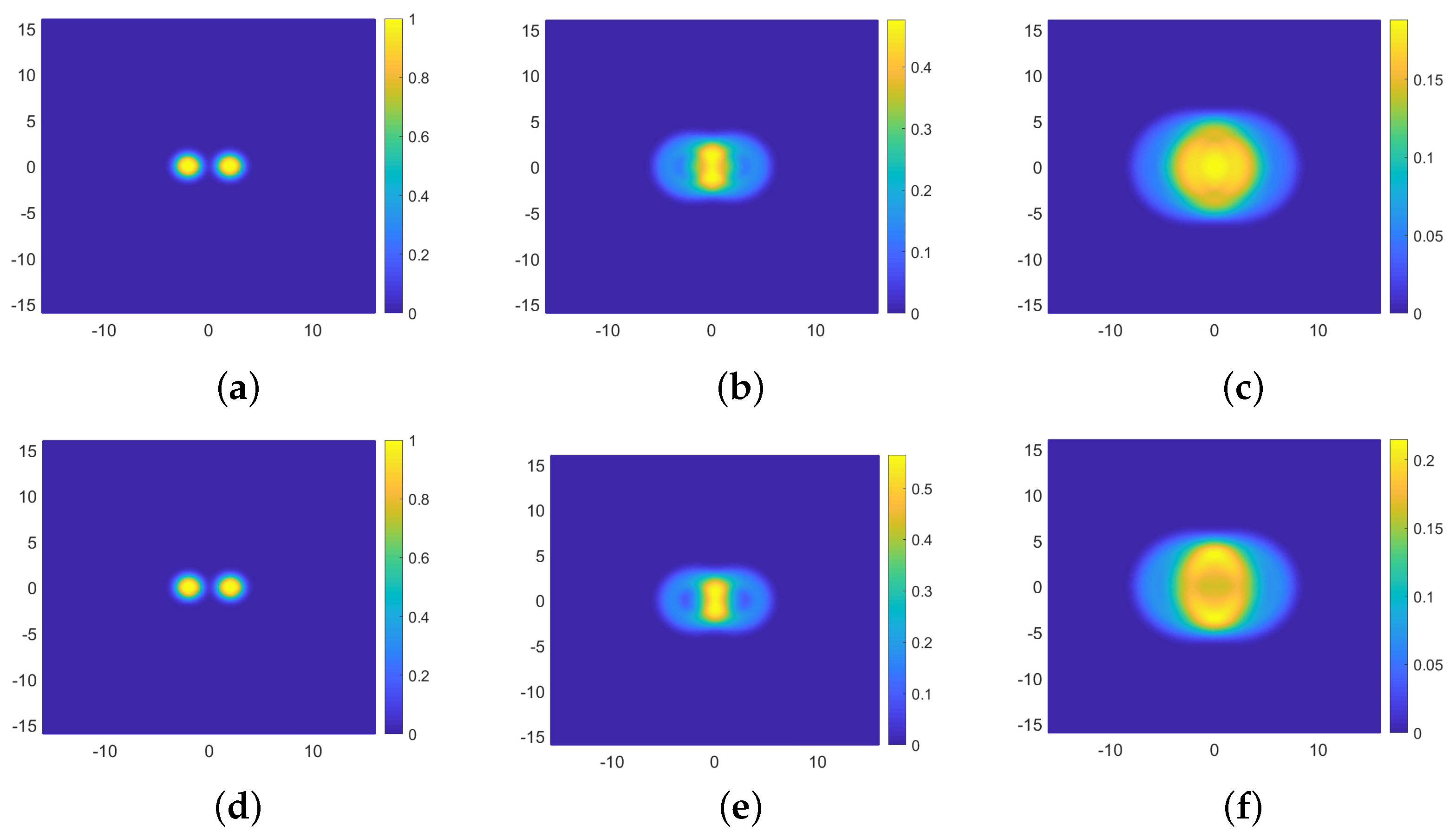
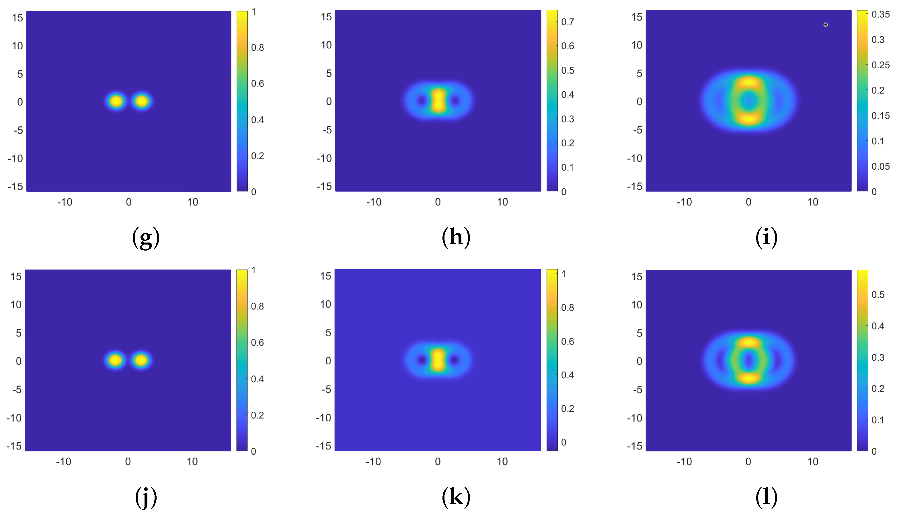
We use the ADI scheme (85)–(88) to obtain the solution of the problem (118). In our simulation, we divided $\mathsf{\Omega }$ into meshes with the space step size of $h=1/8$ and compute the time up to $T=5$ with the time step size $\tau =1/20$.

Figure 1 displays numerical solutions obtained from the ADI scheme (85)–(88) at different moments $t=0$(s), $t=2.5$(s) and $t=5$(s) with various fractional orders $\alpha =1$, $\alpha =1.2$, $\alpha =1.5$, and $\alpha =1.8$. The graphs of initial values for all considered fractional orders are showed to be two spike type in first column of Figure 1. It can be seen that, with time increases, the amplitude of solutions decreases for each fractional order. Moreover, the larger the fractional order $\alpha$ is, the smaller the amplitude of solutions becomes. Numerical results indicate that the fractional order $\alpha$ could play an important role in regulating dynamic of damping.

6. Conclusions

We have developed efficient difference schemes for solving the one- and two-dimensional wave equations with fractional damping. In addition, we have proved the unconditional stability and convergence of the proposed difference schemes. The accuracy of the present difference schemes and the application of the wave equation with fractional damping have been tested in several numerical examples. Numerical simulations show that the values of fractional orders of the Caputo derivative in the damping model have a significant effect on the wave process.

It should be pointed out that the time discretization technique used in this paper is based on the uniform time mesh, which requires strong regularity assumptions. Recent works [18,25,38,39] have discussed the lack of the smoothness near the initial time of the solution of the time-fractional PDEs. Future study will consider the numerical method in a graded time mesh in order to overcome initial time singularity and provide a theoretical basis for the subsequent numerical scheme.

References

- Ma, H.Y.; Yan, B. Nonlinear damping and mass effects of electromagnetic shunt damping for enhanced nonlinear vibration isolation. Mech. Syst. Signal. Process. 2021, 146, 107010. [Google Scholar] [CrossRef]
- Yayla, S.; Cardozo, C.L.; Silva, M.A.J.; Narciso, V. Dynamics of a Cauchy problem related to extensible beams under nonlocal and localized damping effects. J. Math. Anal. Appl. 2021, 494, 124620. [Google Scholar] [CrossRef]
- Choucha, A.; Boulaaras, S.M.; Abdalla, M. Exponential stability of swelling porous elastic with a viscoelastic damping and distributed delay term. J. Funct. Space 2021, 2021, 5581634. [Google Scholar] [CrossRef]
- Chen, G.W. Infinitely many nontrivial periodic solutions for damped vibration problems with asymptotically linear terms. Appl. Math. Comput. 2014, 245, 438–446. [Google Scholar] [CrossRef]
- Liu, C.C.; Meng, F.J.; Zhong, C.K. A note on the global attractor for the weakly damped wave equation. Appl. Math. Lett. 2015, 41, 12–16. [Google Scholar] [CrossRef]
- de Andrade, B.; Tuan, N.H. A non-autonomous damped wave equation with a nonlinear memory term. Appl. Math. Opt. 2022, 85, 36. [Google Scholar] [CrossRef]
- Wang, M.L.; Zhang, J.L.; Li, E.Q.; Xin, X.F. The generalized Cole-Hopf transformation to a general variable coefficient Burgers equation with linear damping term. Appl. Math. Lett. 2020, 105, 106299. [Google Scholar] [CrossRef]
- Yavuz, M.; Sulaiman, T.A.; Usta, F.; Bulut, H. Analysis and numerical computations of the fractional regularized long-wave equation with damping term. Math. Method. Appl. Sci. 2021, 44, 7538–7555. [Google Scholar] [CrossRef]
- Lian, W.; Radulescu, V.D.; Xu, R.Z.; Yang, Y.B.; Zhao, N. Global well-posedness for a class of fourth-order nonlinear strongly damped wave equations. Adv. Calc. Var. 2021, 14, 589–611. [Google Scholar] [CrossRef]
- Ji, B.Q.; Zhang, L.M. A dissipative finite difference Fourier pseudo-spectral method for the Klein-Gordon-Schrödinger equations with damping mechanism. Appl. Math. Comput. 2020, 376, 125148. [Google Scholar] [CrossRef]
- Kirane, M.; Tatar, N.-E. Exponential growth for a fractionally damped wave equation. Z. Anal. Anwend. 2003, 22, 167–177. [Google Scholar] [CrossRef]
- Tatar, N.-E. A blow up result for a fractionally damped wave equation. Nodea-Nonlinear. Diff. 2005, 12, 215–226. [Google Scholar] [CrossRef]
- Charãoa, R.C.; da Luz, C.R.; Ikehata, R. Sharp decay rates for wave equations with a fractional damping via new method in the Fourier space. J. Math. Anal. Appl. 2013, 408, 247–255. [Google Scholar] [CrossRef]
- Yan, Z.; Wang, W.; Liu, X.B. Analysis of a quintic system with fractional damping in the presence of vibrational resonance. Appl. Math. Comput. 2018, 321, 780–793. [Google Scholar] [CrossRef]
- Lokshin, A.A. Wave equation with singular delayed time (in Russian). Dokl. Akad. Nauk. SSSR 1978, 240, 43–46. [Google Scholar]
- Lokshin, A.A.; Rok, V.E. Fundamental solutions of the wave equation with delayed time (in Russian). Dokl. Akad. Nauk. SSSR 1978, 239, 1305–1308. [Google Scholar]
- Wang, Q.F.; Cheng, D.Z. Numerical solution of damped nonlinear Klein-Gordon equations using variational method and finite element approach. Appl. Math. Comput. 2005, 162, 381–401. [Google Scholar] [CrossRef]
- Stynes, M.; O’Riordan, E.; Gracia, J.L. Error analysis of a finite difference method on graded meshes for a time-fractional diffusion equation. SIAM J. Numer. Anal. 2017, 55, 1057–1079. [Google Scholar] [CrossRef]
- Fu, H.F.; Wang, H. A preconditioned fast finite difference method for space-time fractional partial differential equations. Fract. Calc. Appl. Anal. 2017, 20, 88–116. [Google Scholar] [CrossRef]
- Liu, Z.G.; Cheng, A.J.; Li, X.L. A second order Crank–Nicolson scheme for fractional Cattaneo equation based on new fractional derivative. Appl. Math. Comput. 2017, 311, 361–374. [Google Scholar] [CrossRef]
- Ji, C.-C.; Dai, W.; Sun, Z.-Z. Numerical schemes for solving the time-fractional dual-phase-lagging heat conduction model in a double-layered nanoscale thin film. J. Sci. Comput. 2019, 81, 1767–1800. [Google Scholar] [CrossRef]
- Wang, Y.-M.; Zheng, Z.-Y. A second-order L2-1σ Crank-Nicolson difference method for two-dimensional time-fractional wave equations with variable coefficients. Comput. Math. Appl. 2022, 118, 183–207. [Google Scholar] [CrossRef]
- Arshad, S.; Bu, W.P.; Huang, J.F.; Tang, Y.F.; Zhao, Y. Finite difference method for time-space linear and nonlinear fractional diffusion equations. Int. J. Comput. Math. 2018, 95, 202–217. [Google Scholar] [CrossRef]
- Ji, C.-C.; Dai, W. Numerical algorithm with fourth-order spatial accuracy for solving the time-fractional dual-phase-lagging nanoscale heat conduction equation. Numer. Math. Theor. Meth. Appl. 2023, 16, 511–540. [Google Scholar]
- Ji, C.-C.; Qu, W.Z.; Jiang, M.S. Numerical method for solving the fractional evolutionary model of bi-flux diffusion processes. Int. J. Comput. Math. 2023, 100, 880–900. [Google Scholar] [CrossRef]
- Du, N.; Wang, H. A fast finite element method for space-fractional dispersion equations on bounded domains in R2. SIAM J. Sci. Comput. 2015, 37, A1614–A1635. [Google Scholar] [CrossRef]
- Dehghan, M.; Abbaszadeh, M. A finite difference/finite element technique with error estimate for space fractional tempered diffusion-wave equation. Comput. Math. Appl. 2018, 75, 2903–2914. [Google Scholar] [CrossRef]
- Li, C.P.; Chen, A. Numerical methods for fractional partial differential equations. Int. J. Comput. Math. 2018, 95, 1048–1099. [Google Scholar] [CrossRef]
- Li, M.; Huang, C.M.; Ming, W.Y. Mixed finite-element method for multi-term time-fractional diffusion and diffusion-wave equations. Comput. Appl. Math. 2018, 37, 2309–2334. [Google Scholar] [CrossRef]
- Sun, J.; Nie, D.X.; Deng, W.H. A Reduced Finite Element Formulation for Space Fractional Partial Differential Equation. E. Asian J. Appl. Math. 2019, 8, 678–696. [Google Scholar] [CrossRef]
- Liu, Y.Q.; Sun, H.G.; Yin, X.L.; Feng, L.B. Fully discrete spectral method for solving a novel multi-term time-fractional mixed diffusion and diffusion-wave equation. Z. Angew. Math. Phys. 2020, 1, 71. [Google Scholar] [CrossRef]
- Yang, Y.; Chen, Y.P.; Huang, Y.Q.; Wei, H.Y. Spectral collocation method for the time-fractional diffusion-wave equation and convergence analysis. Comput. Math. Appl. 2017, 73, 1218–1232. [Google Scholar]
- Saffarian, M.; Mohebbi, A. Numerical solution of two and three dimensional time fractional damped nonlinear Klein–Gordon equation using ADI spectral element method. Appl. Math. Comput. 2021, 405, 126182. [Google Scholar] [CrossRef]
- Wu, C.; Wei, C.; Yin, Z.; Zhu, A. A Crank-Nicolson Compact Difference Method for Time-Fractional Damped Plate Vibration Equations. Axioms 2022, 11, 535. [Google Scholar] [CrossRef]
- Lyu, P.; Liang, Y.X.; Wang, Z.B. A fast linearized finite difference method for the nonlinear multi-term time-fractional wave equation. Appl. Numer. Math. 2022, 151, 448–471. [Google Scholar] [CrossRef]
- Wang, T.; Jiang, Z.; Zhu, A.; Yin, Z. A Mixed Finite Volume Element Method for Time-Fractional Damping Beam Vibration Problem. Fractal Fract. 2022, 6, 523. [Google Scholar] [CrossRef]
- Sun, Z.Z.; Wu, X.N. A fully discrete difference scheme for a diffusion-wave system. Appl. Numer. Math. 2006, 56, 193–209. [Google Scholar] [CrossRef]
- Lyu, P.; Vong, S. A symmetric fractional-order reduction method for direct nonuniform approximations of semilinear diffusion-wave equations. J. Sci. Comput. 2022, 93, 34. [Google Scholar] [CrossRef]
- Liao, H.-L.; Liu, N.; Lyu, P. Discrete gradient structure of a second-order variable-step method for nonlinear integer-differential models. SIAM J. Numer. Anal. 2023, 61, 2157–2181. [Google Scholar] [CrossRef]
Figure 1.
Effect of damping for different derivatives on peak value at different times. (a) , (b) , (c) , (d) , (e) , (f) , (g) , (h) , (i) , (j) , (k) , (l) .