
A Single-Stack Output Power Prediction Method for High-Power, Multi-Stack SOFC System Requirements

1
School of Information Engineering, Nanchang University, Nanchang 330031, China
2
School of Precision Instrument and Opto-Electronics Engineering, Tianjin University, Tianjin 300072, China
3
Shenzhen Research Institute, Huazhong University of Science and Technology, Shenzhen 518000, China
*
Author to whom correspondence should be addressed.
Inorganics 2023, 11(12), 474; https://doi.org/10.3390/inorganics11120474
Submission received: 9 November 2023
/
Revised: 28 November 2023
/
Accepted: 4 December 2023
/
Published: 6 December 2023
(This article belongs to the Special Issue Advanced Materials and Enhanced Performance of Solid Oxide Fuel Cells/Electrolyzers)
Abstract
:The prediction of stack output power in solid oxide fuel cell (SOFC) systems is a key technology that urgently needs improvement, which will promote SOFC systems towards high-power multi-stack applications. The accuracy of power prediction directly determines the control effect and working condition recognition accuracy of the SOFC system controller. In order to achieve this goal, a genetic algorithm back propagation (GA-BP) neural network is constructed to predict output power in the SOFC system. By testing 40 sets of sample data collected from the experimental platform, it is found that the GA-BP method overcomes the limitation of the traditional back propagation (BP) method—falling into local optima. Further analysis shows that the average relative error of GA-BP has decreased to 1%. The reduction of the relative error improves the accuracy of the prediction results and the average prediction accuracy. Compared with the long short-term memory (LSTM) and BP algorithm, the GA-BP prediction model significantly reduces the relative error of power output prediction, which provides a solid foundation for multi-stack SOFC systems.
1. Introduction
As a representative of electrochemical power generation equipment [1,2], the urgency of fuel cell technology needs and the uncertainty of global energy security are increasing. Scientists around the world are actively seeking clean energy that can achieve optimal conversion efficiency [3,4]. The solid oxide fuel cell (SOFC) has become an attractive option for electricity generation due to its efficient electrochemical power generation reaction and environmentally friendly characteristics, with water as the byproduct [5,6]. In order to enhance its industrialization and promotion, many researchers have developed SOFCs from single-stack to multi-stack systems, and integrated them with other balance of plant (BOP) components, forming an independent power generation system that can adapt to multi-application backgrounds [7,8]. In the current environment, the power distribution of multi-stack systems and the optimization of system efficiency are still unsolved and challenging problems. The premise of solving these problems is to accurately predict the output power of a SOFC stack in the system state [9,10].
In the traditional field of chemistry, modeling is often completed by using mechanism-based approaches. However, the current approach of predicting energy output power and efficiency using mechanism-based models is time-consuming due to the process of mechanism modeling (chemical mechanisms, first-principles equations) and the reliance on software such as Fluent and Aspen for modeling and efficiency prediction. While these models provide accuracy, they are inefficient in terms of modeling and prediction. Additionally, traditional numerical simulations often rely on idealized assumptions; for example, assuming all gases are ideal gases and there is no heat exchange between the system and the surroundings [11]. These assumptions are not suitable for accurately predicting real-time power generation in a SOFC stack. In contrast, constructing data-driven prediction models has the advantage of not requiring detailed knowledge of physical and chemical mechanism equations, thus avoiding the use of modeling software programs with high requirements for computer memory and graphics cards [12]. These models can be built using friendly tools such as MATLAB or Python, and the data-driven methods employed use black-box models, simplifying the technical difficulty.
In the existing field of fuel cell power prediction, the focus often deviates from the system environment. Due to the effective application of backpropagation (BP) and long short-term memory (LSTM) in various fields, their predictive capabilities have been widely recognized [13,14]. Therefore, techniques such as BP and LSTM have been introduced for predicting the operating conditions of fuel cell stacks [15,16], with data sourced from the impedance and temperature of the SOFC stack. These methods tend to perform well in single-input single-output systems but are not suitable for handling strongly coupled and multivariable systems like the SOFC system. Therefore, there is a need to identify new data-driven methods that are applicable to the characteristics of the SOFC system.
Through a literature review, it was found that although the integration of genetic algorithms (GA) and artificial neural networks (ANN) have been widely applied in other fields [17,18], their application in electrochemical systems is still limited. However, it has been observed that they have been successfully used for impedance prediction in proton exchange membrane fuel cells [19]. Additionally, it was found that BP neural networks have been used in the predictive control of the output voltage of a SOFC system and the temperature prediction model of a SOFC system [20,21]. Therefore, this study proposes the use of the GA-BP method to accurately predict the real-time key parameter of power generation in the SOFC stack under system conditions. This method does not require assumptions about problems and conditions like mechanistic modeling, and it can provide predicted operating parameters without complex multi-field coupling condition data and the relationship between different BOP structures.
In addition, in terms of the characteristics of fuel cells: unlike proton-exchange membrane fuel cells SOFCs operate at high temperatures, typically between 800 and 1000 °C [22,23]. The high operating temperature brings about challenges such as temperature fluctuations of external gases, parasitic power losses, and internal material damage, which are difficult to detect in a timely manner. These perturbation factors pose a challenge for accurately predicting the power output of a SOFC system [24,25]. Currently, in the system environment, the data-driven model of SOFCs often involves gas flow rate at the anode and cathode inlets and outlets, load voltage, and stack temperature [26]. However, there still exist discrepancies between these parameters and the requirements of the entire system. It is difficult to arrange sensors for flow rate measurements at the stack inlet and outlet positions in the system environment, and the stack temperature is also difficult to measure due to the instability of the system environment.
Through an extensive review and synthesis of the literature on the construction of prediction models and the key data for SOFC systems, a basic understanding of the research on the prediction of SOFC power generation capacity has been achieved [27,28,29,30]. This paper proposes a novel modeling approach and conducts a comparative study on the power output of SOFC systems. The main innovations of this paper are as follows:
- The prediction for SOFC output power utilizes the combustion chamber temperature, stack temperature, and electrical current as input parameters, with the output power being the output parameter. This approach is more comprehensive than traditional approaches to predictive modeling that rely solely on the inputs and outputs of the stack.
- The suggested GA-BP algorithm notably enhances the precision of output power prediction in a SOFC system, thereby providing valuable references for future investigations on forecasting system operating conditions.
This paper is organized as follows: Section 2 introduces the structural composition of the SOFC system for experimentation; Section 3 proposes a method of using GA to optimize the BP neural network; Section 4 constructs the GA-BP model; Section 5 introduces the data acquisition, processing, and model parameter settings for the experiment; Section 6 compares the prediction results of different models; and the conclusion is presented in Section 7.
2. SOFC System Architecture
The SOFC system used in this experiment is shown in Figure 1. It mainly includes the following parts: SOFC stack, evaporator, reformer, air–exhaust gas heat exchanger, fuel–air heat exchanger, exhaust gas combustion chamber, desulfurizer, dehumidifier, air compressor, air storage tank, electric lighter, cooling water tank, and monitoring system. The fuel used in the experiment is natural gas. In the reformer, natural gas undergoes the following reaction to produce hydrogen gas. The stack used in the system consists of 20 single cells with a size of 13 × 13 cm2, and platinum is used as the catalyst. A typical IV curve of the stack is shown in Figure 2.
The simplified model of the SOFC is shown in Figure 3. In the cold box, water and hydrogen gas are preheated in the evaporator and then introduced into the reformer chamber, and another part of the hydrogen gas is burned with air in the reformer combustion chamber to provide continuous high-temperature conditions for the reforming reaction. In the hot box, the air–exhaust gas heat exchanger exchanges heat between the high-temperature waste gas from the exhaust combustion chamber and the cold cathode air just introduced into the system to increase the temperature of the cathode air, so that the temperature of the cathode air increases to about 600 °C after the first heat exchange. The role of the fuel–air heat exchanger is to exchange heat between the reformed high-temperature fuel and the cathode air after the first heat exchange, in order to reduce the temperature difference between the anode gas and the cathode air.
3. Problem Description and Methodology
3.1. Problem Description
The SOFC system is characterized by the presence of high-temperature and low-temperature regions. Consequently, determining the operating conditions is challenging, and the system exhibits a high level of complexity [31]. As a result, accurately predicting the output power becomes a difficult task. Neural networks have been widely employed for predicting the output power of SOFCs due to their superior accuracy in handling a complex system compared to traditional methods. However, existing neural network models often suffer from lengthy training times and a tendency to become trapped in local minima, which leads to deviations from the actual situation and hampers the accurate prediction of SOFC output power. Therefore, substantial improvements and rigorous testing are necessary to achieve more precise prediction outcomes.
3.2. Methodology
To enhance the accuracy of predicting the output power of SOFCs and mitigate the potential issue of local optima, the utilization of GA is employed as a means to optimize the initial weight and threshold of the neural network, thereby minimizing the impact of random initial weight and threshold values on the final solution. Based on the enhanced GA-BP, a prediction model is developed with the purpose of forecasting the output power of SOFC. During the construction of the neural network architecture, the training dataset is utilized for model training and performance evaluation. By comparing the mean square error (MSE) and number of iterations of the prediction model established with varying numbers of hidden layer neurons, the optimal number of hidden layer neurons for the prediction model is selected. This would result in an improvement in the precision and dependability of the prediction model. Subsequently, the prediction model is established after identifying the most suitable number of hidden layer neurons. Finally, the test dataset is inputted to the model to obtain the predicted output. The assessment of the prediction model’s accuracy and reliability involves an analysis and comparison of the discrepancies between the predicted values generated by the model and the actual values.
4. Model Building
4.1. BP Neural Network
The BP neural network is a neural network architecture consisting of three or more layers and numerous neurons. These layers include the input layer, hidden layer, and output layer [32,33]. The BP neural network is advantageous in complex system analyses due to its ability to learn rules through training and generate output values that closely match the desired results without the need for predetermined mathematical equations. This makes it particularly effective in handling nonlinear function relationships. Nonetheless, it is important to acknowledge that the BP neural network has certain limitations. For instance, it is susceptible to getting trapped in local minimums during the training process, which can hinder its accuracy and reliability. Additionally, the training outcomes of the BP neural network are heavily influenced by the initial random weights. It further limits the accuracy and reliability in predicting the output power of a SOFC system.
4.2. Genetic Algorithm
GA is a highly effective and parallelized approach that serves as a global search method. It was designed to replicate the process of biological evolution found in nature. This algorithm possesses the ability to autonomously acquire and accumulate information about the search space as it progresses, and it can dynamically adjust its control to ultimately obtain the optimized solution for the given problem [34].
Compared to traditional optimization methods such as enumeration algorithm and heuristic algorithm, GA is based on biological evolution. It offers several advantages, including good convergence, shorter calculation time, and high robustness, especially when high calculation accuracy is needed. The outstanding advantage of GA is global optimization [35]. The algorithm possesses the ability to efficiently explore the entirety of the solution space, avoiding the common pitfall of becoming trapped in a local optimal solution. The schematic diagram of GA is shown in Figure 4.
4.3. GA-BP Algorithm Model
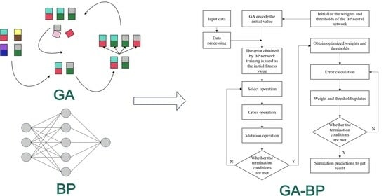
The training process of the BP neural network is susceptible to the problem of becoming trapped in local minima. This paper proposes integrating GA with the neural network to optimize the BP neural network. The objective is to establish a prediction model for SOFC output power based on GA-BP. This method utilizes the global search capability of GA to optimize the initial weights and thresholds, thereby overcoming these limitations. The flowchart depicting the GA-BP algorithm is presented in Figure 5 The specific steps are as follows [36]:
- Choice of encoding
For GA, there are two common types of encoding, namely real number encoding and binary encoding. The binary encoding method is computationally intensive as it requires frequent encoding and decoding operations. It also has the significant disadvantage of being prone to the Hamming Cliff, which makes the cross and mutation operation difficult. Therefore, the real number encoding method is selected for the GA of the SOFC system output power prediction model.
- 2.
- Population initialization
Population initialization is the process of creating an initial group of individuals that serve as the initial population for an algorithm prior to its execution. This procedure involves the establishment of the size of the population, the determination of the evolution times, the determination of the generation gap between the parent strings and their offspring strings, and the determination of the probabilities of both crossover and mutation at the individual level. Individuals are potential solutions for a given problem. In this experiment, the individuals are represented by chromosome strings in real coding form and can undergo operations such as crossover, mutation, and selection. By calculating the fitness value of individuals, individuals with smaller errors can be found. Subsequently, the weights and thresholds are assigned to the BP neural network.
- 3.
- Initialize the BP neural network model
This paper utilizes a neural network model comprising three layers. The selection of the number of neurons in each layer is determined through an analysis of the training data set from the SOFC system. Empirical Equation (1) determines the number of neurons in the hidden layer:
In the Equation, k denotes the quantity of neurons present in the hidden layer. m represents the quantity of neurons in the input layer, that is, the number of parameters considered as input parameters in the SOFC system data. Similarly, n represents the quantity of neurons in the output layer, that is, the number of parameters considered as output parameters in the SOFC system data. Additionally, the variable l is a constant value that is constrained within the range [0, 1].
- 4.
- Designing the Fitness Function
The GA relies on fitness functions to optimize and assess data. Consequently, the efficacy of GA is intricately linked to the construction of the fitness function. Since the probability of survival is determined by the fitness function, it is imperative that its value is positive, thereby promoting competition among individuals. Typically, the fitness value function is designed based on the optimization objective function. Since the SOFC output power prediction model requires the prediction output to have high accuracy, the objective function chosen for this experiment is the MSE between the predicted values and the true values. The MSE function is represented by Equation (2):
In the Equation, the variable n is the number of training samples. The variables yi and oi represent the actual value of the neurons and the predicted output of the neurons, respectively. In the output power prediction model of the SOFC system, yi is the true value of SOFC system output power, and oi is the predicted value of the output power. Additionally, the coefficient k is defined as 1/n.
Since the GA selects individuals with higher fitness function values, the fitness value function uses the reciprocal of the mean square error. This is shown in Equation (3):
In this way, individuals with higher fitness values are those with smaller mean square error functions, so the population can evolve towards better values.
- 5.
- Selection operation
The primary aim of the selection operation is to identify and select individuals with superior traits that can be transmitted to future generations through the operation of crossover and mutation, either directly or indirectly. In determining the selection operation, the fitness of individuals is a crucial factor in the output power prediction model of the SOFC system. The likelihood of selection is positively correlated with a higher fitness. Individuals who possess lower fitness are more susceptible to being eliminated. The relative fitness is defined using the roulette wheel method. This is shown in Equation (4):
Among them, p(xi) is the relative fitness of individual xi, which indicates the probability of that individual being selected. Meanwhile, f(xi) is the original fitness of an individual, and is the cumulative fitness of the population.
According to the probability of each individual’s choice, denoted as p(xi), the roulette wheel is divided into N sectors. Equation (5) represents the central angle of the i-th sector:
Then, a pointer is set on the roulette wheel. When a selection is made, one can envision a spinning roulette wheel. If the pointer points to the nth sector after the wheel stops, the individual is selected as shown in Figure 6.
- 6.
- Cross operation
Cross operation is a process in which two individuals are randomly chosen from a given population, and their chromosomes are exchanged and combined. This procedure facilitates the transmission of the favorable attributes of the parent strings to the offspring strings, resulting in the production of new individuals with superior traits. The process of performing a cross operation between the i chromosome ai and the j chromosome aj at position r, is illustrated by Equation (6):
The equation includes a random number, represented as b, that takes on values ranging from 0 to 1.
- 7.
- Mutation operation
To mitigate the risk of GA converging to a suboptimal solution within the optimization procedure, so as to improve the accuracy of SOFC system output power prediction, the incorporation of mutation is imperative to introduce variability among individuals throughout the search process. In this process, i genes of individual j are selected for mutation, resulting in a completely new individual, as shown in Equation (7):
In this Equation, amax and amin represent the maximum and minimum values of the gene aij, respectively. r2 represents a random number, with a value ranging between [0, 1]. g denotes the current iteration number, while Gmax represents the maximum number of evolutions. Additionally, r is another random number, with a value ranging between [0, 1].
- 8.
- Calculate fitness
In order to evaluate the fitness of a new individual, it is necessary to substitute the original chromosome with a new chromosome. If the resulting fitness value satisfies the specified condition, proceed to step 9. If not, return to step 4 to continue the fitness calculation process.
- 9.
- Termination criterion:
- a.
- Reach the maximum number of iterations.
- b.
- The current best solution has either remained unchanged or changed very little for several consecutive steps.
- c.
- The algorithm has found an acceptable best solution, achieving the performance goal.
- 10.
- Train
When one of the conditions in step 9 is met, the BP neural network is assigned optimized weights and thresholds. Subsequently, the network undergoes training using the training set until the set error is achieved.
5. Model Settings
5.1. Data Sample
Data samples are obtained at fixed intervals after the start of the power generation process from the parameter repository of the SOFC system. The collected data samples include four key parameters, namely combustion chamber temperature, stack temperature, electrical current magnitude, and output power. In this paper, the first three are taken as input parameters, and output power is taken as the output parameter to establish the SOFC output power prediction model based on GA-BP. In the collected data, the temperature range of the combustion chamber is 750–850 °C, the temperature range of the stack is 650–700 °C, the electrical current magnitude range is 17–22 A, and the output power is between 280 and 480 W.
In order to enhance the precision and comprehensiveness of the prediction, this paper partitions the gathered 240 datasets. A total of 200 sets are randomly chosen as the training sets for the prediction model, while the remaining 40 sets are set aside as the test sets. In order to ensure a smooth convergence of the model training process, each parameter needs to be normalized. This paper utilizes max–min normalization. The equation for the normalization transformation is presented in Equation (8):
In the Equation, xmax and xmin are the maximum and minimum values of the sample data, respectively. x and x* are the values before and after normalization, respectively. Reverse normalization is performed after obtaining the experimental results to obtain the true value.
5.2. Parameter Settings of BP and GA-BP
In this paper, three input parameters and one output parameter were chosen. Therefore, the neural network in this paper has been configured with three neurons in the input layer and one neuron in the output layer. Figure 7 depicts the neural network architecture. Therefore, according to Equation (1) for the hidden layer, the number of neurons in the hidden layer can be any integer between three and twelve. When the number of hidden layer neurons is insufficient, it will lead to underfitting and low model accuracy. If the number of neurons is too high, it tends to lead to overfitting and distortion. To minimize the influence of the neural network structure on the precision of predictions, we replaced different odd numbers ranging from three to twelve as the number of neurons in the hidden layer. By comparing the mean square error and the number of iterations across different schemes, we can select an appropriate number of hidden layer neurons for the GA-BP model. The comparison results of different schemes for the number of hidden layer neurons before inverse normalization are shown in Table 1.
As shown in Table 1, in the range of three to twelve neurons, there is an observed pattern of initially decreasing and subsequently increasing MSE. As the number of neurons increases, the number of iterations tends to decrease. In order to ensure the number of iterations and prediction accuracy of the overall model, the number of neurons in the hidden layer is finally selected as five.
In the model, the GA parameters are set as follows: the size of the population is 50, the probability of crossover and mutation is 0.8 and 0.05, respectively. The maximum number of evolutions is 50, and the generation gap is 0.9. The training parameters for the BP neural network are as follows: the training times are set to 1000, the activation function is set to tansig, the learning rate is 0.01, the training goal is 0.0001. Network training utilizes the Levenberg–Marquardt (LM) algorithm. Table 2 shows the parameter settings.
6. Results and Discussion
The GA-BP model is constructed to test the accuracy of the model prediction by using the toolbox in the MATLAB platform. Figure 8 displays the prediction results. Figure 9 displays the fit curve and prediction intervals at the 95% confidence level. The relative error is shown in Figure 10 and Table 3.
As shown in Figure 8, the yellow column represents the predicted output power of the GA-BP model, and the red dot represents the true value. It can be seen that for the 40 test sample points, the predicted values of GA-BP are approximate to the true values, indicating the accuracy of the GA-BP prediction model.
As shown in Figure 9a, the blue dashed line represents the fit curve of the predicted output power of the GA-BP model, and the two orange solid lines represent the prediction interval at a 95% confidence level. It can be seen that the R2 of the GA-BP model is 0.9832, indicating a strong correlation between the predicted value of GA-BP and the true value. Furthermore, it can be observed that out of the forty test sample points, only one point is outside the prediction interval, indicating a low likelihood of the predicted value deviating from the true value, and in most cases, the predicted values are close to the true values.
As shown in Table 3 and the purple column in Figure 10, the relative errors of the predicted values of the GA-BP model for each test sample point are presented. It can be seen that for most of the test sample points, the relative error is within a very small range, indicating that constructing a GA-BP model to predict the output power of the SOFC system has high accuracy.
LSTM is a special type of recurrent neural network (RNN) designed to address the issues of gradient vanishing and exploding during the training of long sequences [37]. LSTM captures and processes long-term dependencies in time series by introducing a gate control mechanism and cell states. The BP neural network is a feedforward network in which the output depends solely on the current input, without a gate control mechanism and cell states. Furthermore, there are differences in their training processes. LSTM uses the backpropagation through time (BPTT) method to handle time series data, while BP uses the backpropagation algorithm for training. GA-BP is based on the BP neural network, and it introduces GA to optimize the weights and thresholds in order to obtain better solutions.
To demonstrate the accuracy of using the GA-BP model to predict the output power of SOFC systems, the BP model and LSTM model were constructed using the MATLAB platform. The same data set as the GA-BP model was used for training and prediction, and the results were compared. The parameter settings of the BP model are consistent with those of the BP parameter settings in the GA-BP model, and the partial parameter settings of the LSTM model are shown in Table 4. Figure 8 displays the prediction results. Figure 9 displays the fit curves and prediction intervals at the 95% confidence level. The relative error is shown in Figure 10 and Table 3.
As shown in Figure 8, the predicted values of these two models are not as close to the true values as the GA-BP model. As shown in Figure 9, among the fit curves of the three models, the R2 of the GA-BP model is greater than these two models. Furthermore, as shown in Table 3 and Figure 10, the relative error of the predicted values of the GA-BP model is also smaller in most cases than these two models.
In addition, the MSE, R2, maximum relative error, minimum relative error, average error, and training duration of the three models are shown in Table 5.
As shown in Table 5, the MSE, maximum error, minimum error, and average error of the GA-BP model’s prediction results are also smaller than the other two models, indicating the accuracy of the GA-BP prediction model.
These experimental results suggest that the three models possess the ability to predict the output to some extent. However, in comparison to the conventional BP algorithm model, the prediction accuracy of the GA-BP algorithm model exhibits a significant improvement. This enhancement can be attributed to the fact that the BP algorithm model generates random initial weights and thresholds, and employs gradient descent to optimize the loss function, resulting in the obtained solution being confined to a locally optimal solution. On the other hand, in the GA-BP model, the initial weights and thresholds of the network are optimized by GA, thereby circumventing the local optimization of the obtained solution and substantially enhancing the accuracy of prediction.
In order to further validate the effectiveness of the GA-BP model in this experiment, a new set of 40 samples was selected. Then, the trained neural network was used to predict the output power and the results were compared with the actual values. An analysis of the predicted results is shown in Table 6.
From the data in Table 6, it is not difficult to see that the prediction results of this model remain accurate even for new values outside the range of the original sample data.
Based on the research results of this article, the proposed GA-BP prediction model for a single-stack SOFC system output power has certain effectiveness and application value. Moreover, since SOFC systems often integrate multiple stacks, it also provides guidance for predicting the output power of high-power multi-stack SOFC systems.
7. Conclusions
In high-power SOFC systems, multiple stacks are inevitable, and the output power of multiple stacks directly affects system efficiency. Due to a lack of relevant experience, this article starts with predicting the power output of a single stack in order to provide guidance for multi-stack systems. SOFC output power is influenced by several key parameters, including stack temperature, combustion chamber temperature, and electrical current magnitude. By considering these three key input parameters and the output power as the output parameter, the optimal number of hidden layer neurons can be selected by empirical equation and experimental method to create the BP neural network. Then, the BP model is optimized by GA, and the GA-BP model is established to improve the prediction accuracy. The results obtained from the testing samples show that the prediction model is both stable and reliable. Compared with the traditional BP prediction model, the R2 of the enhanced GA-BP prediction model increases from 0.9573 to 0.9832. In addition, the MSE decreases from 92.67 to 35.94, the maximum relative error decreases from 15.068% to 9.724%, the minimum relative error decreases from 0.043% to 0.021%, and the average relative error value decreases from 1.7% to 1%. Meanwhile, compared to the various indicators of the LSTM prediction results, it also demonstrates superior performance. The reduction of these relative errors helps to improve the accuracy of the average prediction results. The high-precision prediction and modeling of stack output power in the SOFC system provides an important basis for the development of high-power multi-stack SOFC systems in the future.
Author Contributions
Conceptualization, J.H. and D.Z.; methodology, D.Z.; software, W.Z.; validation, J.H. and W.Z.; formal analysis, D.Z. and Z.G.; investigation, M.L.; resources, J.H., D.Z. and W.Z.; data curation, M.L. and Z.G.; writing—original draft preparation, D.Z.; writing—review and editing, J.H., W.Z. and M.L.; visualization, W.Z. and X.W.; supervision, J.H.; project administration, D.Z. and J.H.; funding acquisition, D.Z., X.W. and J.H. All authors have read and agreed to the published version of the manuscript.
Funding
This research was funded by the National Natural Science Foundation of China (grant No. 62203204 and No. 12364036), the Jiangxi Provincial Natural Science Foundation (grant No. 20232BAB201046, No. 20232BAB202028, and No. 20212BAB212013), and the College Students’ Innovative Entrepreneurial Training Plan Program of China (grant No. 202210403096 and No. 202210403098).
Data Availability Statement
The data presented in this study are available on request from the corresponding author.
Conflicts of Interest
The authors declare no conflict of interest.
References
- Onn, T.M.; Küngas, R.; Fornasiero, P.; Huang, K.; Gorte, R.J. Atomic Layer Deposition on Porous Materials: Problems with Conventional Approaches to Catalyst and Fuel Cell Electrode Preparation. Inorganics 2018, 6, 34. [Google Scholar] [CrossRef]
- Suchaneck, G.; Artiukh, E. Nonstoichiometric Strontium Ferromolybdate as an Electrode Material for Solid Oxide Fuel Cells. Inorganics 2022, 10, 230. [Google Scholar] [CrossRef]
- Pirou, S.; Talic, B.; Brodersen, K.; Hauch, A.; Frandsen, H.L.; Skafte, T.L.; Persson, A.H.; Hogh, J.V.T.; Henriksen, H.; Navasa, M.; et al. Production of a monolithic fuel cell stack with high power density. Nat. Commun. 2022, 13, 1263. [Google Scholar] [CrossRef] [PubMed]
- Ahmed, K.I.; Ahmed, M.H. Developing a Novel Design for a Tubular Solid Oxide Fuel Cell Current Collector. Appl. Sci. 2022, 12, 6003. [Google Scholar] [CrossRef]
- Pan, Z.; Liu, J.; Liu, J.; Ning, X.; Qin, Z.; He, L. Active Disturbance Rejection Optimization Control for SOFCs in Offshore Wind Power. Appl. Sci. 2023, 13, 3364. [Google Scholar] [CrossRef]
- Wu, X.-L.; Zhang, H.; Liu, H.; Xu, Y.-W.; Peng, J.; Xia, Z.; Wang, Y. Modeling Analysis of SOFC System Oriented to Working Condition Identification. Energies 2022, 15, 1804. [Google Scholar] [CrossRef]
- Zhou, J.; Wang, Z.; Han, M.; Sun, Z.; Sun, K. Optimization of a 30 kW SOFC combined heat and power system with different cycles and hydrocarbon fuels. Int. J. Hydrog. Energy 2022, 47, 4109–4119. [Google Scholar] [CrossRef]
- Marocco, P.; Gandiglio, M.; Santarelli, M. When SOFC-based cogeneration systems become convenient? A cost-optimal analysis. Energy Rep. 2022, 8, 8709–8721. [Google Scholar] [CrossRef]
- Zhou, A.; Li, X.-S.; Ren, X.-D.; Song, J.; Gu, C.-W. Thermodynamic and economic analysis of a supercritical carbon dioxide (S-CO2) recompression cycle with the radial-inflow turbine efficiency prediction. Energy 2020, 191, 116566. [Google Scholar] [CrossRef]
- Yabanova, I.; Kecebas, A. Development of ANN model for geothermal district heating system and a novel PID-based control strategy. Appl. Therm. Eng. 2013, 51, 908–916. [Google Scholar] [CrossRef]
- Jin, F.Y.; Xiong, C.; Zhou, H.F.; Huang, Y.Q. Predictive control simulation of solid oxide fuel cells based on an artificial bee colony-support vector machine (abc-svm) model. J. B. Univ. Chem. Technol. 2021, 48, 96–104. [Google Scholar] [CrossRef]
- Yarullin, D.N.; Zavalishin, M.N.; Gamov, G.A.; Lukanov, M.M.; Ksenofontov, A.A.; Bumagina, N.A.; Antina, E.V. Prediction of Sensor Ability Based on Chemical Formula: Possible Approaches and Pitfalls. Inorganics 2023, 11, 158. [Google Scholar] [CrossRef]
- Al-Nader, I.; Lasebae, A.; Raheem, R.; Khoshkholghi, A. A Novel Scheduling Algorithm for Improved Performance of Multi-Objective Safety-Critical Wireless Sensor Networks Using Long Short-Term Memory. Electronics 2023, 12, 4766. [Google Scholar] [CrossRef]
- Singpai, B.; Wu, D. Using a DEA–AutoML Approach to Track SDG Achievements. Sustainability 2020, 12, 10124. [Google Scholar] [CrossRef]
- Wang, S.; Zhang, N.; Wu, L.; Wang, Y. Wind speed forecasting based on the hybrid ensemble empirical mode decomposition and GA-BP neural network method. Renew. Energy 2016, 94, 629–636. [Google Scholar] [CrossRef]
- Ren, L.; Dong, J.; Wang, X.; Meng, Z.; Zhao, L.; Deen, M.J. A Data-Driven Auto-CNN-LSTM Prediction Model for Lithium-Ion Battery Remaining Useful Life. IEEE Trans. Industr. Inform. 2021, 17, 3478–3487. [Google Scholar] [CrossRef]
- Chen, K.; Laghrouche, S.; Djerdir, A. Aging prognosis model of proton exchange membrane fuel cell in different operating conditions. Int. J. Hydrog. Energy 2020, 45, 11761–11772. [Google Scholar] [CrossRef]
- Huo, H.; Chen, J.; Wang, K.; Wang, F.; Jin, G.; Chen, F. State Estimation of Membrane Water Content of PEMFC Based on GA-BP Neural Network. Sustainability 2023, 15, 9094. [Google Scholar] [CrossRef]
- Petrone, R.; Zheng, Z.; Hissel, D.; Péra, M.C.; Pianese, C.; Sorrentino, M.; Becherif, M.; Yousfi-Steiner, N. A review on model-based diagnosis methodologies for PEMFCs. Int. J. Hydrog. Energy 2013, 38, 7077–7091. [Google Scholar] [CrossRef]
- Li, M.; Chen, Z.; Dong, J.; Xiong, K.; Chen, C.; Rao, M.; Peng, Z.; Li, X.; Peng, J. A Data-Driven Fault Diagnosis Method for Solid Oxide Fuel Cell Systems. Energies 2022, 15, 2556. [Google Scholar] [CrossRef]
- Zhang, Y.; Zhang, Y.Y.; Hou, G.L.; Fan, P.P.; IEEE. Research on BP algorithm-based SOFC system temperature model. In Proceedings of the 2015 Chinese Automation Congress (CAC), Wuhan, China, 27–29 November 2015; pp. 1932–1935. [Google Scholar] [CrossRef]
- Wu, X.-L.; Xu, Y.-W.; Li, D.; Zheng, Y.; Li, J.; Sorrentino, M.; Yu, Y.; Wan, X.; Hu, L.; Zou, C.; et al. Afterburner temperature safety assessment for solid oxide fuel cell system based on computational fluid dynamics. J. Power Sources 2021, 496, 229837. [Google Scholar] [CrossRef]
- Wu, X.-L.; Xu, Y.-W.; Zhao, D.-Q.; Zhong, X.-B.; Li, D.; Jiang, J.; Deng, Z.; Fu, X.; Li, X. Extended-range electric vehicle-oriented thermoelectric surge control of a solid oxide fuel cell system. Appl. Energy 2020, 263, 114628. [Google Scholar] [CrossRef]
- Cheng, H.; Li, X.; Jiang, J.; Deng, Z.; Yang, J.; Li, J. A nonlinear sliding mode observer for the estimation of temperature distribution in a planar solid oxide fuel cell. Int. J. Hydrog. Energy 2015, 40, 593–606. [Google Scholar] [CrossRef]
- Zhang, L.; Jiang, J.; Cheng, H.; Deng, Z.; Li, X. Control strategy for power management, efficiency-optimization and operating-safety of a 5-kW solid oxide fuel cell system. Electrochim. Acta 2015, 177, 237–249. [Google Scholar] [CrossRef]
- Rao, M.; Wang, L.; Chen, C.; Xiong, K.; Li, M.; Chen, Z.; Dong, J.; Xu, J.; Li, X. Data-Driven State Prediction and Analysis of SOFC System Based on Deep Learning Method. Energies 2022, 15, 3099. [Google Scholar] [CrossRef]
- Oryshchyn, D.; Harun, N.F.; Tucker, D.; Bryden, K.M.; Shadle, L. Fuel utilization effects on system efficiency in solid oxide fuel cell gas turbine hybrid systems. Appl. Energy 2018, 228, 1953–1965. [Google Scholar] [CrossRef]
- Selvam, K.; Komatsu, Y.; Sciazko, A.; Kaneko, S.; Shikazono, N. Thermodynamic analysis of 100% system fuel utilization solid oxide fuel cell (SOFC) system fueled with ammonia. Energy Convers. Manag. 2021, 249, 114839. [Google Scholar] [CrossRef]
- Thai-Quyen, Q.; Van-Tien, G.; Lee, D.K.; Israel, T.P.; Ahn, K.Y. High-efficiency ammonia-fed solid oxide fuel cell systems for distributed power generation. Appl. Energy 2022, 324, 119718. [Google Scholar] [CrossRef]
- Meng, T.; Cui, D.; Ji, Y.L.; Cheng, M.J.; Tu, B.F.; Lan, Z.L. Optimization and efficiency analysis of methanol SOFC-PEMFC hybrid system. Int. J. Hydrog. Energy 2022, 47, 27690–27702. [Google Scholar] [CrossRef]
- Yang, J.; Qin, S.; Zhang, W.Y.; Ding, T.F.; Zhou, B.; Li, X.; Jian, L. Improving the load-following capability of a solid oxide fuel cell system through the use of time delay control. Int. J. Hydrog. Energy 2017, 42, 1221–1236. [Google Scholar] [CrossRef]
- Ruan, X.M.; Zhu, Y.Y.; Li, J.; Cheng, Y. Predicting the citation counts of individual papers via a BP neural network. J. Informetr. 2020, 14, 101039. [Google Scholar] [CrossRef]
- Yang, A.M.; Zhuansun, Y.X.; Liu, C.S.; Li, J.; Zhang, C.Y. Design of Intrusion Detection System for Internet of Things Based on Improved BP Neural Network. IEEE Access 2019, 7, 106043–106052. [Google Scholar] [CrossRef]
- Qu, Z.; Liu, H.; Wang, Z.; Xu, J.; Zhang, P.; Zeng, H. A combined genetic optimization with AdaBoost ensemble model for anomaly detection in buildings electricity consumption. Energy Build. 2021, 248, 111193. [Google Scholar] [CrossRef]
- Kuang, T.; Hu, Z.Y.; Xu, M.H. A Genetic Optimization Algorithm Based on Adaptive Dimensionality Reduction. Math. Probl. Eng. 2020, 2020, 8598543. [Google Scholar] [CrossRef]
- Liu, K.L.; Lin, T.; Zhong, T.T.; Ge, X.R.; Jiang, F.C.; Zhang, X. New methods based on a genetic algorithm back propagation (GABP) neural network and general regression neural network (GRNN) for predicting the occurrence of trihalomethanes in tap water. Sci. Total Environ. 2023, 870, 161976. [Google Scholar] [CrossRef]
- Wentz, V.H.; Maciel, J.N.; Gimenez Ledesma, J.J.; Ando, O.H., Jr. Solar Irradiance Forecasting to Short-Term PV Power: Accuracy Comparison of ANN and LSTM Models. Energies 2022, 15, 2457. [Google Scholar] [CrossRef]
Figure 1.
The SOFC system.

Figure 2.
Typical IV curve of the stack.

Figure 3.
Schematic diagram of the SOFC system.

Figure 4.
Schematic diagram of the GA.

Figure 5.
GA-BP neural network flowchart.

Figure 6.
Roulette method.

Figure 7.
BP neural network topology diagram.

Figure 8.
Prediction results.

Figure 9.
Fit curves and prediction intervals at the 95% confidence level. (a) GA-BP prediction model. (b) BP prediction model. (c) LSTM prediction model.
Figure 9.
Fit curves and prediction intervals at the 95% confidence level. (a) GA-BP prediction model. (b) BP prediction model. (c) LSTM prediction model.

Figure 10.
Prediction relative errors.


Table 1.
Performance comparison of different numbers of neurons.
| Hidden Layer Neuron | MSE | Iterations |
|---|---|---|
| 3 | 0.00061 | 20 |
| 5 | 0.00052 | 17 |
| 7 | 0.00074 | 16 |
| 9 | 0.00085 | 15 |
| 11 | 0.00085 | 14 |
Table 2.
Parameter settings.
| Parameter of BP | Setting |
| Training times | 1000 |
| Neurons in the input layers | 3 |
| Neurons in the hidden layers | 5 |
| Neurons in the output layers | 1 |
| Activation function | tansig |
| Training function | LM |
| Learning rate | 0.1 |
| Training goal | 0.0001 |
| Parameter of GA | Setting |
| Size of the population | 50 |
| Maximum number of evolutions | 50 |
| Crossover probability | 0.8 |
| Mutation probability | 0.05 |
| Generation gap | 0.9 |
Table 3.
Prediction relative error for the three models.
| Sample | GA-BP/% | BP/% | LSTM/% | Sample | GA-BP/% | BP/% | LSTM/% |
|---|---|---|---|---|---|---|---|
| 1 | 0.194 | 0.546 | 1.278 | 21 | 0.305 | 0.277 | 0.929 |
| 2 | 0.678 | 0.095 | 1.072 | 22 | 0.389 | 0.678 | 0.595 |
| 3 | 0.141 | 0.043 | 0.196 | 23 | 0.142 | 0.201 | 0.24 |
| 4 | 2.826 | 3.444 | 3.128 | 24 | 0.041 | 0.331 | 0.129 |
| 5 | 1.721 | 0.565 | 1.658 | 25 | 9.724 | 15.068 | 11.053 |
| 6 | 0.461 | 1.652 | 1.431 | 26 | 0.224 | 6.14 | 2.859 |
| 7 | 1.189 | 0.239 | 0.631 | 27 | 1.292 | 0.452 | 0.709 |
| 8 | 0.269 | 0.603 | 1.821 | 28 | 1.998 | 2.248 | 2.049 |
| 9 | 0.622 | 1.553 | 1.246 | 29 | 1.63 | 2.335 | 2.271 |
| 10 | 1.085 | 0.794 | 0.137 | 30 | 0.359 | 0.499 | 0.192 |
| 11 | 0.867 | 2.703 | 0.876 | 31 | 0.353 | 1.247 | 0.323 |
| 12 | 0.884 | 1.669 | 0.983 | 32 | 0.286 | 1.282 | 0.344 |
| 13 | 1.598 | 2.189 | 0.641 | 33 | 0.121 | 0.505 | 0.108 |
| 14 | 0.75 | 0.095 | 1.57 | 34 | 0.737 | 1.164 | 1.839 |
| 15 | 0.439 | 0.184 | 1.186 | 35 | 0.517 | 1.443 | 1.438 |
| 16 | 0.578 | 0.488 | 0.14 | 36 | 0.021 | 1.385 | 1.09 |
| 17 | 1.052 | 1.523 | 0.837 | 37 | 0.345 | 0.276 | 0.522 |
| 18 | 2.822 | 4.207 | 2.801 | 38 | 0.035 | 1.575 | 2.027 |
| 19 | 1.476 | 1.556 | 1.903 | 39 | 0.282 | 2.45 | 2.286 |
| 20 | 1.345 | 2.09 | 2.445 | 40 | 0.213 | 2.175 | 1.517 |
Table 4.
Parameter settings of LSTM.
| Parameter | Setting |
|---|---|
| Batch size | 30 |
| Neurons in the input layers | 3 |
| Number of hidden layers | 1 |
| Neurons in the hidden layers | 16 |
| Neurons in the output layers | 1 |
| Learning rate | 0.01 |
| Training times | 1000 |
| Optimizer | Adam |
Table 5.
Analysis and comparison of the prediction results.
| MSE | R2 | Maximum Error | Minimum Error | Average Error | Training Duration | |
|---|---|---|---|---|---|---|
| BP | 92.67 | 0.9573 | 15.068% | 0.043% | 1.7% | 4 s |
| GA-BP | 35.94 | 0.9832 | 9.724% | 0.021% | 1% | 83 s |
| LSTM | 56.50 | 0.9733 | 11.053% | 0.108% | 1.5% | 61 s |
Table 6.
Analysis of prediction results.
| MSE | R2 | Maximum Error | Minimum Error | Average Error | |
|---|---|---|---|---|---|
| GA-BP | 43.82 | 0.9805 | 4.325% | 0.032% | 1.3% |
Disclaimer/Publisher’s Note: The statements, opinions and data contained in all publications are solely those of the individual author(s) and contributor(s) and not of MDPI and/or the editor(s). MDPI and/or the editor(s) disclaim responsibility for any injury to people or property resulting from any ideas, methods, instructions or products referred to in the content. |
© 2023 by the authors. Licensee MDPI, Basel, Switzerland. This article is an open access article distributed under the terms and conditions of the Creative Commons Attribution (CC BY) license (https://creativecommons.org/licenses/by/4.0/).
Share and Cite
MDPI and ACS Style
Zhang, D.; Hu, J.; Zhao, W.; Lai, M.; Gao, Z.; Wu, X. A Single-Stack Output Power Prediction Method for High-Power, Multi-Stack SOFC System Requirements. Inorganics 2023, 11, 474. https://doi.org/10.3390/inorganics11120474
AMA Style
Zhang D, Hu J, Zhao W, Lai M, Gao Z, Wu X. A Single-Stack Output Power Prediction Method for High-Power, Multi-Stack SOFC System Requirements. Inorganics. 2023; 11(12):474. https://doi.org/10.3390/inorganics11120474
Chicago/Turabian StyleZhang, Daihui, Jiangong Hu, Wei Zhao, Meilin Lai, Zilin Gao, and Xiaolong Wu. 2023. "A Single-Stack Output Power Prediction Method for High-Power, Multi-Stack SOFC System Requirements" Inorganics 11, no. 12: 474. https://doi.org/10.3390/inorganics11120474
Note that from the first issue of 2016, this journal uses article numbers instead of page numbers. See further details here.