Field Analysis of Stepwise Effective Thermal Conductivity along a Borehole Heat Exchanger under Artificial Conditions of Groundwater Flow

Abstract

Heat advection caused by groundwater flow can potentially improve the performance of a borehole heat exchanger. However, the required flow velocity is not achieved under most natural conditions. This study focuses on artificial groundwater flow generated by pumping and investigates the associated effect in a lowland area near the Toyohira River alluvial fan, Sapporo, Japan. Thermal response test results are compared under natural and artificial groundwater flow conditions. A pumping well is constructed one meter from the borehole. Temperature profiles are measured in the U-tube during testing, using a pair of optic fiber distributed temperature sensors. The effective thermal conductivity is calculated from the profiles obtained in each 10-m sub-layer; this thermal conductivity is termed the stepwise thermal conductivity. Additionally, the upward flow velocity in the pumping well is measured to estimate the mean groundwater flow velocity at the borehole. The results show that effective thermal conductivity increases at depths less than 50 m, where the pumping creates mean velocities greater than 0.1 m d⁻¹ in each sub-layer (1.5 md⁻¹ on average). Thus, a borehole length of 50 m is more reasonable at the test site for its efficiency in a ground source heat pump system coupled with the pumping well than that used.

1. Introduction

Ground source heat pump systems (GSHPs) have been increasingly established for heating and air conditioning in residences and commercial buildings owing to their energy efficiency, ubiquitous availability, and environmental friendliness [1,2]. Among a variety of ground heat exchangers, closed loop borehole heat exchangers (BHEs) are the most widely used. BHEs consist of a high-density polyethylene U-tube(s) in a vertical borehole of a depth of approximately 100 to 300 m. The performance of a BHE in a GSHP is dependent on the effective thermal conductivity around the BHE. The effective thermal conductivity is variable, with ranges between <1 W m⁻¹ K⁻¹ in unsaturated fine sediments and >3 W m⁻¹ K⁻¹ in dense consolidated rocks [3]. In addition, the effective thermal conductivity may increase in aquifers with groundwater flow velocities sufficiently high for heat advection relative to the conduction, i.e., the Peclet number is of order 1 in principle [4]. Several numerical studies have indicated that the threshold of the groundwater flow velocity for the advection effect is commonly on the order of 0.1 md⁻¹ [5]. The threshold velocity was also evaluated on the same order by other numerical studies [6,7,8]. Such high velocities of groundwater flow are limited to cases in which both hydraulic gradients and conductivities are relatively high, such as in unconsolidated gravelly aquifers beneath steep slopes [4]. Therefore, the design and planning of GSHPs typically do not take into account the groundwater flow effect on the performance of a BHE.

This study focuses on the artificial groundwater flow effect generated by pumping water from a well adjacent to a BHE. The pumping causes radial groundwater flow, and the flow velocity increases as the pumping rate increases. In addition, when the BHE is close to the pumping well and the groundwater flow velocity exceeds the threshold at the BHE, the effective thermal conductivity around the BHE increases; thus, the performance of the GSHP improves. The effect of artificial groundwater flow can differ depending on the pumping conditions (i.e., well depth and pumping rate) and on the hydrogeologic conditions (i.e., sedimentary structure and hydraulic conductivity in each layer). Thus, field measurements and analyses are required to evaluate the effect of artificial groundwater flow for the design and planning of GSHPs at each site.

The objective of this study is to obtain field evidence of the effect of artificial groundwater flow on the effective thermal conductivity around a BHE, based on thermal response tests (TRTs). TRT was originally developed in Sweden [9] to determine the average effective thermal conductivity along a BHE. The standard analysis is valuable for practitioners in terms of its simplicity under the assumption of an infinite line heat source. The methodology is summarized in texts such as ASHRAE [10] and IEA [11]. The analysis method has been also developed by using analytical solutions of finite line heat source [12,13], inversion techniques [14], Monte-Carlo method [15] and numerical simulations [5,6,7,8,16]. Especially in this study, the standard TRT is limited because the averaged effective thermal conductivity is insensitive to the geologic structure under the ground [16]. In order to address the limitation, our pervious study [17] measured and analyzed temperatures in a U-tube during the TRT, resulting in effective thermal conductivity in each 10-m thickness sub-layer; this variation is termed the stepwise effective thermal conductivity.

This study performs the multi-layer concept TRTs under two different conditions of groundwater flow. One is the natural condition without pumping, and the other is the artificial condition with pumping from a water well. The test site is located in a lowland area near the Toyohira River alluvial fan, Sapporo, Japan. The natural flow velocity is moderate on the flat slope, but pumping from the gravelly aquifers increases the groundwater flow velocity. The water well is located one meter from the BHE. The temperature of heat transfer fluid is measured in the U-tube during the testing using a pair of fiber optic distributed temperature sensors (DTSs). The effective thermal conductivity is estimated on the line heat source analysis, indicating apparent increases of the stepwise effective thermal conductivity due to the advection effect. This study also measures the upward flow velocity in the pumping well and estimates the mean groundwater flow at the BHE for comparison with the stepwise effective thermal conductivity. This study shows the actual effect of artificial groundwater flow and discusses a reasonable BHE length in terms of efficiency for GSHPs under the artificial conditions.

2. Materials and Methods

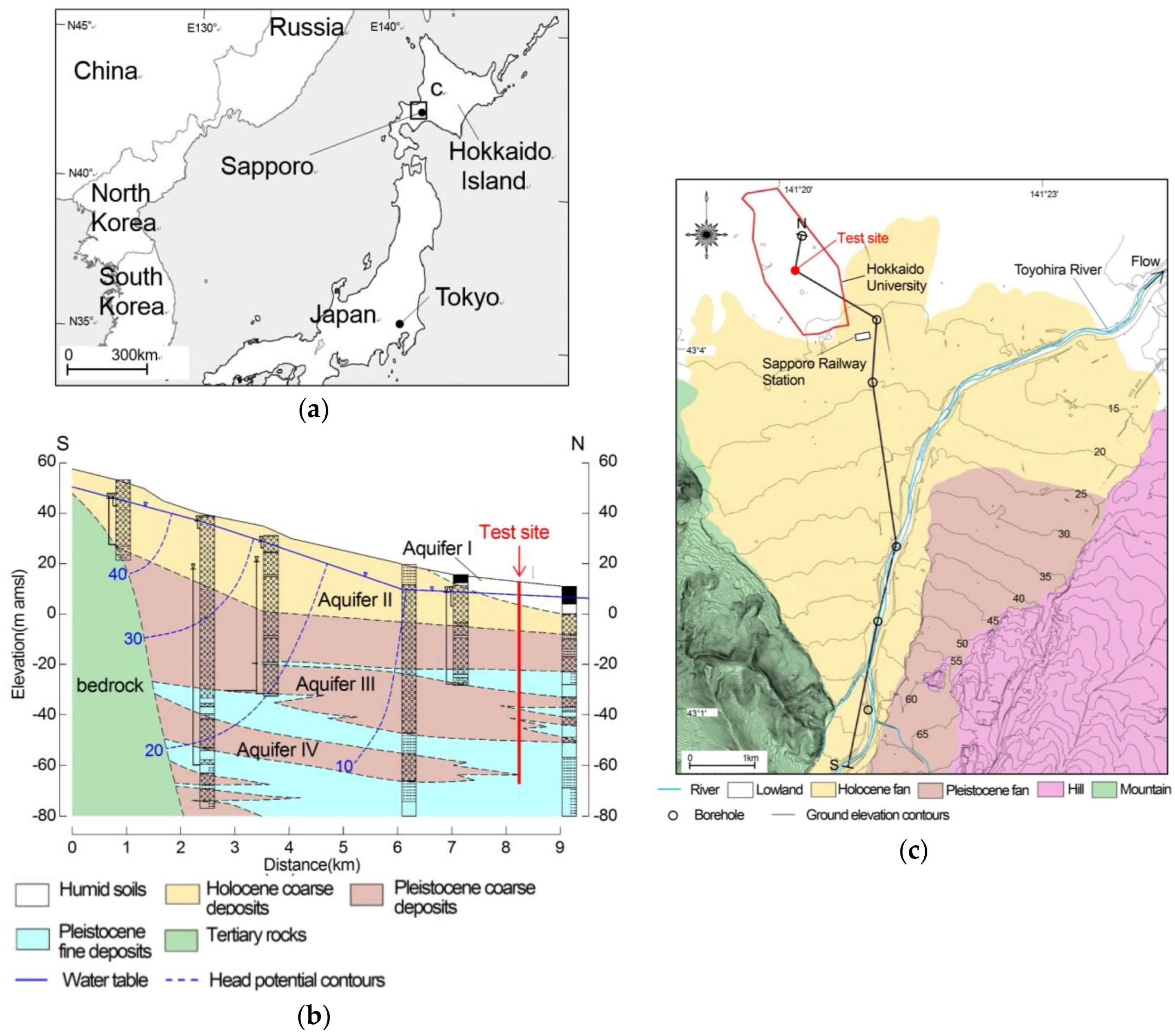
2.1. Site Description

Figure 1a,b illustrate maps of the test site at regional and local scales, respectively. The test site is located at 43°03′06″ N and 141°15′25″ E at Hokkaido University, Sapporo, Japan. Sapporo is a capital city in the northern island of Japan, Hokkaido, and has been developed on and around the Toyohira River alluvial fan. Figure 1b shows that the alluvial fan is surrounded topographically by mountains to the northwest, hills to the northeast, and lowlands to the south. The radius of the fan is approximately 7 km, and the area is approximately 31 km². The fan consists of a western Holocene fan and an eastern Pleistocene fan [18]. The Holocene fan contains the subsurface groundwater reservoir. The test site is located on the lowlands near the alluvial fan. The topographic slope of the lowland area is less than 1%; thus, the groundwater flow velocity is moderate for BHE performance.

Figure 1c shows a geologic cross section along a longitudinal line (the black line in Figure 1b). Tertiary rocks can be observed beneath the riverbed at the fan head, but the fan basement suddenly inclines northward to a depth of several hundreds of meters. Because of this depression, various Quaternary sediments underlie the central to distal parts of the fan, with a thickness of hundreds of meters. The unconsolidated formation is classified hydrogeologically into Aquifers I–IV [19]. The deepest aquifer, Aquifer IV, is composed of alternating clay, sand, and gravelly layers and formed before the alluvial fan. The Pleistocene, Aquifer III, and Holocene, Aquifer II, aquifers consist mainly of alluvial fan gravel deposits, i.e., poorly sorted sandy gravel sediments. The total thickness of the gravel aquifers is more than 100 m at the middle of the fan. The boundary of Aquifers III and II is generally not obvious from the available borehole data. Aquifer I is distributed only near the ground level in the fan toe, and it consists of fine materials related to the fan recession. Figure 1c also shows the water table level and the potentiometric head contours in the cross section. In the upper fan (<6 km in distance), the hydraulic head decreases in the downstream and downward directions, reflecting the three-dimensional groundwater flow system.

The test site is located 8 km from the southern edge of the cross section. Figure 1c shows that the formation at the test site is composed of Aquifers I–IV. The water table is close to the surface (approximately several meters deep), and the hydraulic gradient is less than 1% under natural conditions. However, pumping from gravelly Aquifers II and III increases the velocity of groundwater flow around the BHE.

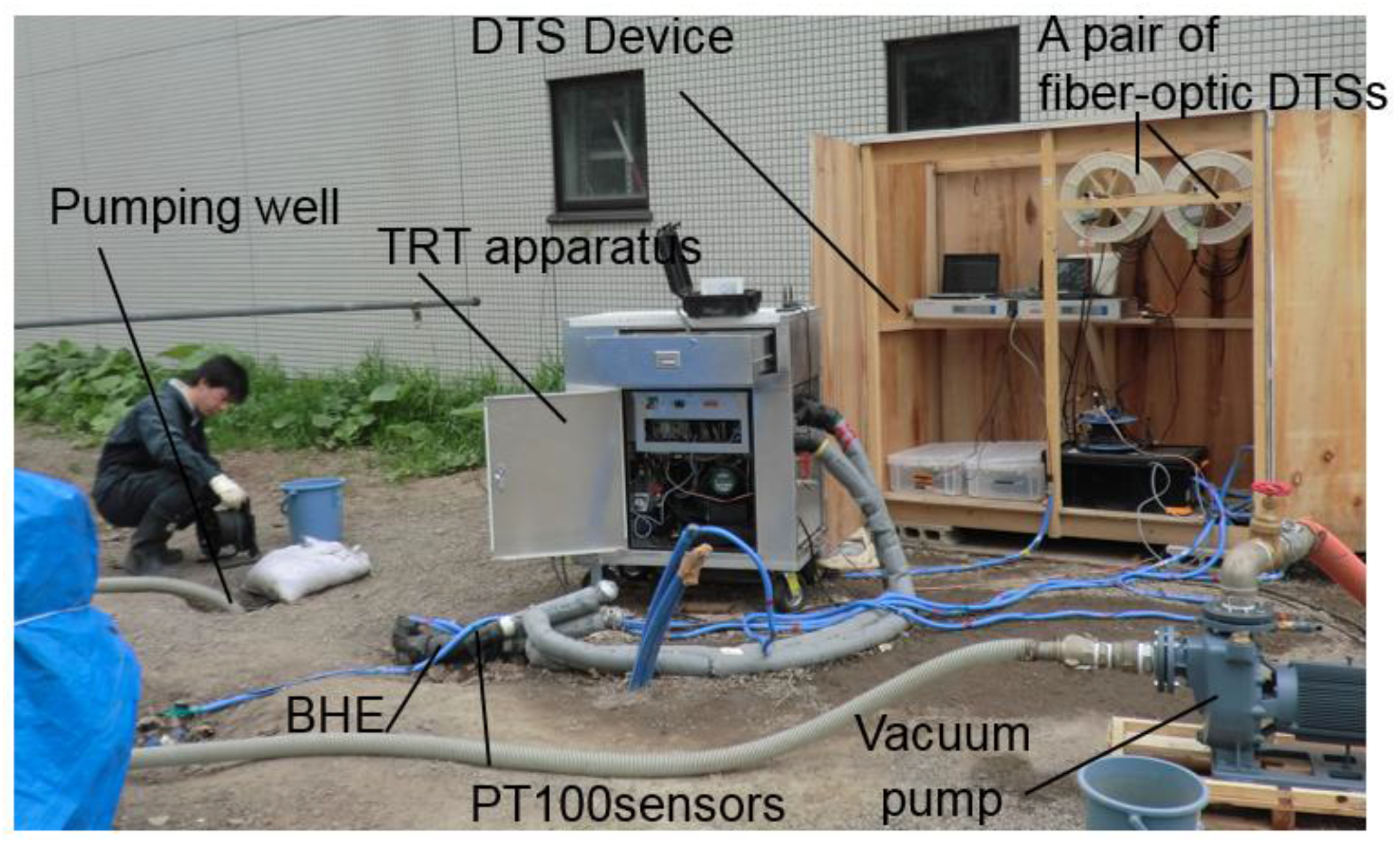
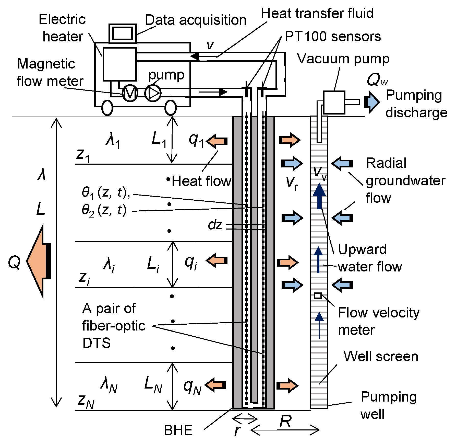
2.2. Thermal Response Tests under Natural and Artificial Conditions of Groundwater Flow

This study performed standard TRTs as follows: (1) a BHE with configurations (diameter, length, and U-tube(s)) similar to those planned is constructed for testing; (2) the U-tube contains the heat carrier fluid (water or brine); (3) the fluid is circulated at a constant rate in the U-tube; (4) the heat is injected into the fluid at a constant rate; (5) the fluid temperatures are measured during the heating at both ends of the U-tube; and (6) the temperature measurements are analyzed to determine the average effective thermal conductivity along the BHE and the thermal resistance within the BHE.

In addition to the standard TRT, this study measured the temperature of the heat transfer fluid in the U-tube by installing a pair of fiber optic DTSs. One DTS is installed in the inlet tube, and the other DTS is installed in the outlet tube. The DTSs were used to measure temperatures at multiple points along a distance of several kilometers based on the Raman scattering effect of the laser pulse of the optic fibers [21]. Notably, the diameter of each fiber sensor was sufficiently small to avoid disturbances due to flow circulation; thus, the DTSs could be used to monitor and investigate the GSHP system [22]. The temperature measurements by the DTSs were also used to match the analytical solutions by the numerical inversion techniques, resulting in the depth-varying effective thermal conductivity of soils [23] and the thermal resistances of BHEs [24].

The test configuration is illustrated in Figure 2. A photo of the TRT is also shown in Figure 3. The BHE was constructed at a depth of L = 80 m using a double-casing driller in February 2015. The BHE was composed of a single U-tube (ID = 25 mm and OD = 32 mm), which was buried with silica sand as the grout material. Tap water was enclosed in the U-tube under a pressure greater than 0.1 MPa. The water well was constructed with the same depth and at a distance of R = 1 m from the BHE in May 2016. The water well included a plastic screen (ID = 75 mm) and silica sand between the screen and the ground. After construction, the water well was flushed via upward pumping until the discharge water was sufficiently clear.

This study performed TRTs at the BHE without pumping from the water well (the first TRT) and with pumping at a constant rate (the second TRT). In both TRTs, the configurations were the same, excluding pumping and non-pumping. The total heating rate via the electric heater was Q = 5.2 kW during the period of 60 h. The flow rate for circulating the heat transfer fluid was constant at v = 0.00033 m³ s⁻¹ (20 L/min). The temperatures of the fluid at the ends of U-tube were observed using PT100 platinum resistance thermometers, which have an accuracy of 0.1 K. The temperatures of the fluid in the U-tube θ₁(z, t) and θ₂(z, t) were observed using the DTSs. The DTS specifications are shown in

Table 1. Distributed temperature sensor (DTS) device and sensor specifications.

Instrument	N4385A-008 (A.P. Sensing, Ltd)
Maximum distance range	8 km
Spatial resolution	0.5 m
Measurement interval	1 min
Accuracy (Uncertainty)	+/− 0.2 K (moving average per 20 min)
Optic fiber	SKF-VP13L404CC140 (NK Systems, Ltd.)
Structure	Dual fibers in a single water-proofed tube
Diameter	4 mm (18 mm at the top)
Total length	140 m
Temperature range	−10 °C to 85 °C

. The sensors were able to reduce the random errors by alternating the laser pulse emitted in the forward and backward directions. In addition, offset calibration and a moving average were performed to reduce the standard deviations of temperature fluctuations within 0.2 K [17]. The first TRT was performed from 28 April to 1 May 2016. The second TRT was performed during 10–20 May 2016 at a constant pumping rate of Q_v = 0.0053 m³/s (320 L/min) using a centrifugal vacuum pump. The extraction mouth for pumping was set at a depth of 6 m (2.3 m below the water table). The total displacement of the water table was 1.7 m at the end of pumping (t = 60 h).

This study also measured the upward flow velocity toward the extraction mouth in the pumping well during the second TRT. The measurement was performed every 0.5 m in depth using an in-hole micro-flowmeter, Model 3216, Oyo Co., Ltd., Tokyo, Japan. The device measured the number of propeller rotations in the pumping well, which was translated to the flow velocity. The groundwater discharge per unit depth was based on the upward flow through the meter. This study calculated the mean groundwater flow velocity at the location of the BHE based on the assumption of a circular flow field. First, the radial flow discharge into the well per unit depth was calculated as a product of the vertical slope of the upward velocity measurements and the cross-sectional area of the well (0.0088 m²). Next, the mean groundwater flow velocity was calculated as the discharge divided by 2πr (the distance r at the BHE is one meter).

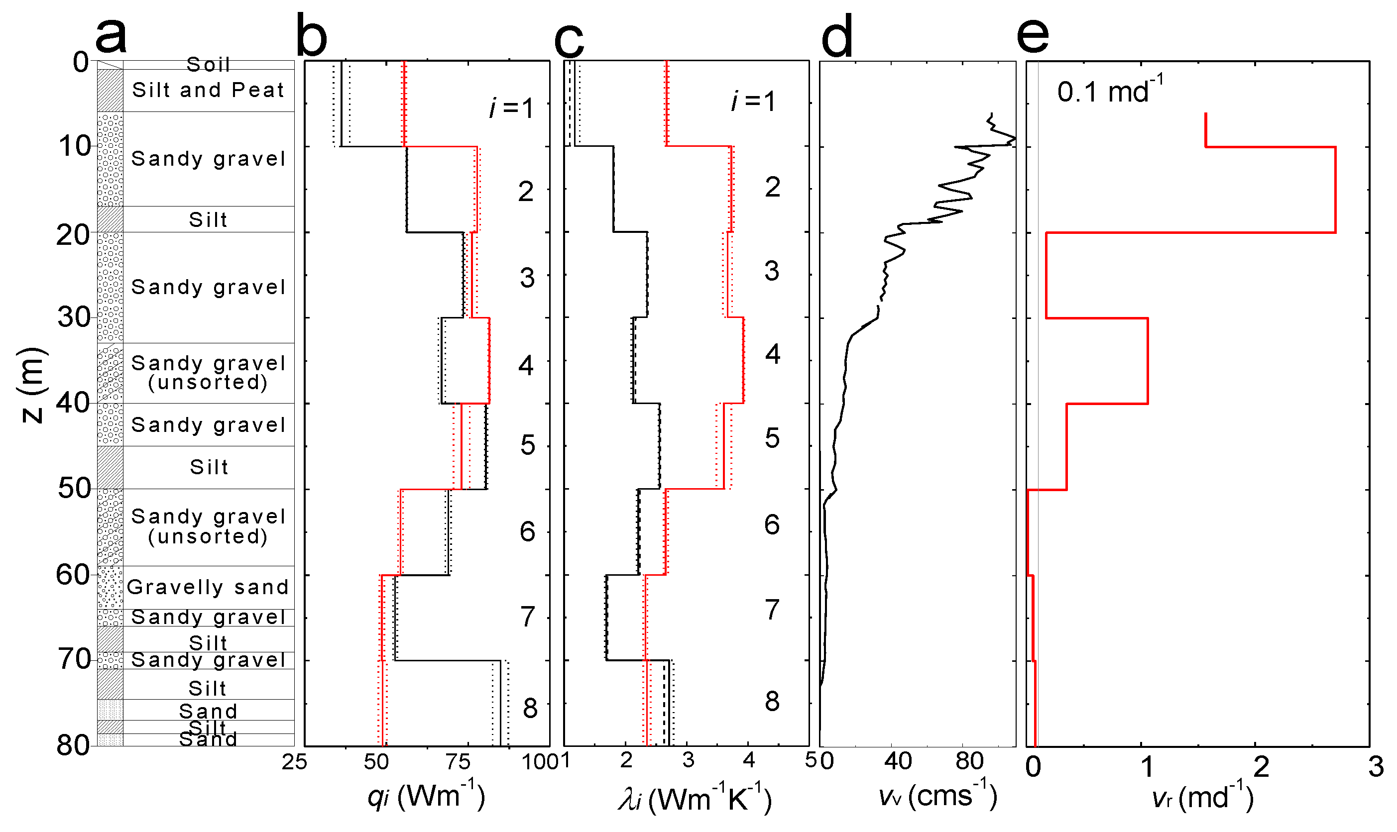
2.3 Analysis of Temperature Profiles to Determine Stepwise Thermal Conductivity

In the standard TRT, the temperature measurements of the heat transfer fluid at the ends of the U-tube were analyzed based on the assumption that the BHE was the line heat source of uniform heat injection along the length of a finite region of homogeneity. The approximate solution of the temperature around the BHE due to the heating process was obtained as follows [25]:

$$\overline{\theta }-{\theta }_0\approx \frac{q}{4\pi \lambda }(-\ln \frac{r^2}{4\alpha t}-\gamma )+q{R}_{\mathrm{b}},$$

(1)

where $\overline{\theta }$ is average temperature surrounding the BHE (K), θ₀ is the initial temperature of the ground (K), q is the heat exchange rate per unit depth (W m⁻¹), r is the radius of the BHE (m), λ is the depth-averaged ground thermal conductivity (W m⁻¹ K⁻¹), α is the thermal diffusivity (m² h⁻¹), γ is Euler’s constant (≃ 0.5772), t is the elapsed time since the start of heating (h), and R_b is the thermal resistance of the BHE (m KW⁻¹). Equation (1) shows that the temperature displacement increases linearly on a log scale of elapsed time t during the testing. When the temporal temperature slope is assumed constant, the effective thermal conductivity λ is calculated using two factors: the heat exchange rate per unit depth q and the temporal temperature slope:

$$\lambda =\frac{q}{4\mathsf{\pi }{k}_{\mathrm{t}}},$$

(2)

where k_t is the temporal slope of the temperature on a log scale of elapsed time t (K). The slope is estimated from the average temperatures of the circulating fluids via manual fitting upon visual inspection or linear regression fitting. q is also calculated by dividing the total heat exchange rate Q (W) by the total length of the BHE. The total heat exchange rate was calculated as follows:

$$Q=C_s\rho v\Delta \theta ,$$

(3)

where C_s is the specific heat of the heat transfer fluids (J kg⁻¹), ρ is the fluid density (kg m⁻³), and v is the flow rate (m³ s⁻¹). λ is determined in Equation (2), and R_b is calculated based on Equation (1) as follows:

$$R_{\mathrm{b}}=\frac{{\theta }_{\mathrm{intersect}}-{\theta }_0}{q}-\frac{1}{4\pi \lambda }(\ln \frac{4\alpha }{r^2}-\gamma ),$$

(4)

where θ_intersect is the intersect of the linear fitting line of temperature displacements at the elapsed time t = 1 h on a logarithmic scale. It should be considered that the estimates are influenced by uncertainty in related to measurement and parameterization errors, resulting in the theoretical errors in TRTs are on the order of 5% for effective thermal conductivity and 10-15% for the thermal resistance [26].

This study extended the analytical approach based on the line heat source theory to a horizontally stratified formation, as shown in Figure 2. The formation consisted of N sub-layers. The effective thermal conductivity was constant at λ_i within each layer but different among layers. The heat exchange rate was also constant at q_i throughout each layer during the TRT. L_i and z_i are the thickness and the boundary depth, respectively, of the ith layer. The depth-averaged conductivity λ_i was assumed equal to λ in Equation (2) [27]. Thus, Equation (2) was transformed as follows:

$${\lambda }_i=\frac{q_i}{4\mathsf{\pi }{k}_{\mathrm{t}i}},i=1,2,\cdots ,N,$$

(5)

where λ_i is the individual effective thermal conductivity in the ith layer (W m⁻¹ K⁻¹), q_i is the heat exchange rate per unit depth in the ith layer (W m⁻¹), and k_ti is the temporal temperature slope of elapsed time on a logarithm scale (K).

In each sub-layer, the heat exchange rate was estimated from the sum of the temperature displacements in the inflow and downflow tubes. Although the displacements were directly calculated in the standard TRT using the temperature displacement between the temperature measurements in the ends of the U-tube, as shown in Equation (3), the proposed method calculates the temperature displacements as the vertical slope of the sequential temperature data:

$$q_i=q_i^{(\mathrm{in})}+q_i^{(\mathrm{out})}=c\rho v(\Delta {\theta }_i^{\left(\mathrm{in}\right)}+\Delta {\theta }_i^{\left(\mathrm{out}\right)})/L_i\cong c\rho v(-k_{\mathrm{z}i}^{\left(\mathrm{in}\right)}+k_{\mathrm{z}i}^{\left(\mathrm{out}\right)}),$$

(6)

where k_zi⁽ⁱⁿ⁾ and k_zi^(out) are the vertical slopes of sequential temperature data in the inflow and outflow paths, respectively, of the ith layer. The temperature measurements recorded by the DTSs fluctuated more and were less accurate than those recorded by conventional temperature sensors, such as PT100 sensors. Thus, the vertical slopes of the sequential temperature data effectively reduced the measurement uncertainty in a statistical sense. The vertical temperature slopes were calculated at each elapsed time based on a linear regression analysis of the sequential data within each vertical segment. The heat exchange rate was calculated using Equation (6) at each measurement time (every one minute in this study) and was averaged during the heating period in each sub-layer. The average rates were used as inputs into Equation (5) to calculate the individual conductivities λ_i. This study also calculated the standard deviations of q_i and the ranges of λ_i to evaluate the uncertainty in this analysis.

The line heat source analysis was based on the minimum elapsed time required to transform the original error function into a logarithmic function and the maximum time required to approach steady state rather than radial heat conduction [11]. This study analyzed the temperature data during the heating period between t = 12 h and 60 h, as recommended in [28]. Additionally, in this analysis, the thickness in each sub-layer should be assigned to validate the line heat source assumption. Although the BHE in each sub-layer has a limited length, the temperatures based on the finite line source model were practically the same with those based on the infinite line source when the vertical length was about 10 m (40 feet) [25]. As a field study [17], our previous study conducted in Asahikawa City, Hokkaido, Japan, indicated that the effective thermal conductivity was approximately constant when the thickness was at least 10 m. Thus, this study assumed that the thickness required to validate the line heat source assumption was constant at 10 m, and the formation around the BHE (L = 80 m) was assumed to consist of 8 sub-layers of 10 m in thickness. The DTS measurement interval was dz = 0.5 m. Temperature data recorded at 21 depths were used for the regression analysis of q_i and k_ti in each sub-layer. This study also calculated the total heat exchange rate Q* from q_i and the average effective thermal conductivity λ* from λ_i. Additionally, Q* and λ* were compared with the standard test results based on Q in Equation (3) and λ in Equation (2).

3. Results and Discussion

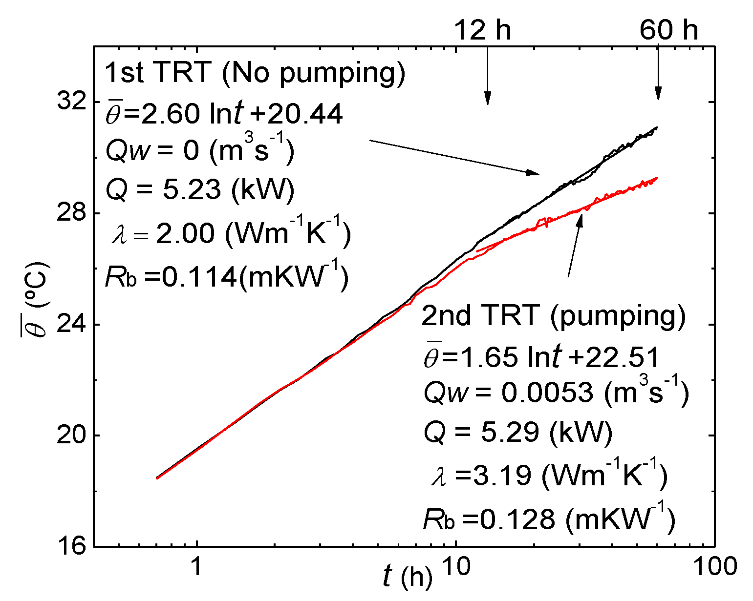
3.1. Standard Test Results

Figure 4 shows the average fluid temperatures $\overline{\theta }$ measured by the PT100 sensors and the fitted lines for the determination of k_t based on Equation (2). The measurement data set is included in the excel file as the supplementary material. The temperatures in the first and second TRTs increased during the heating process. The temperature increase was almost the same during both TRTs until the elapsed time of approximately t = 10 h because heating was dominant in the borehole. After approximately t = 10 h, the temperature increase was smaller in the second TRT than that in the first TRT. The relatively small increase in the second TRT was due to the heat advection caused by artificial groundwater flow. The average effective thermal conductivity λ was calculated using Equation (2). In the first TRT, λ = 2.00 W m⁻¹ K⁻¹, which is that of ‘Light sand and 15% water’ in Table 5 of Chapter 34 in [10]. In the second TRT, average effective thermal conductivity was λ = 3.19 W m⁻¹ K⁻¹, which was almost 1.6 times larger than that during the first TRT. Additionally, the thermal resistance value of the BHE was calculated using Equation (4). In the first TRT, R_b = 0.114 m KW⁻¹, and R_b = 0.128 m KW⁻¹ during the second TRT, were almost the same in terms of an error criterion of R_b as described above (10%–15%), and were reasonable based on Table 6 in [10].

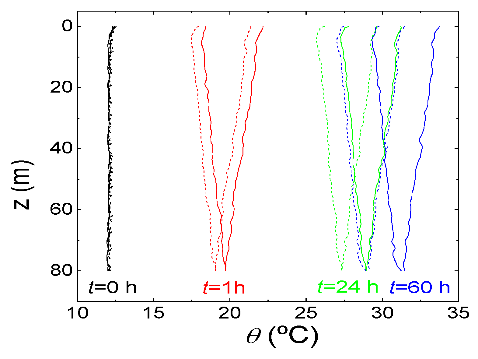
3.2. Profiles of Temperature in the U-Tube

Figure 5 shows the temperature profiles in the U-tube at extracted elapsed times (t = 0, 1, 24, and 60 h) during the first and the second TRTs for examples of the DTS measurements. The profile data are also included in the supplementary material. At the initial time (t = 0 h), the temperatures were constant at 12 °C in both the inlet and outlet tubes as a result of fluid circulation without heating for approximately 0.5 h before the tests. The temperature profiles were almost the same between the first and second TRTs after heating at t = 1 h because the heating domain was limited within the borehole, as described above. At t = 24 h and 60 h, there were differences in the temperature profiles between the first and second TRTs. The average temperature differences along the BHE were one kelvin at t = 12 h and two kelvin at t = 60 h. These differences were due to the effect of artificial groundwater flow into the pumping well.

3.3. Comparison of Stepwise Thermal Conductivity under Natural and Artificial Conditions of Groundwater Flow

Table 2. Summary of the TRT results under natural (first) and artificial (second) conditions.

First TRT (no pumping)					Second TRT (pumping)
1Qw	0				0.0053
2Q	5.23				5.29
3Q*	5.20				5.16
4λ	2.00				3.19
5λ*	2.08				3.12
6i	7zi	8qi	9kti	10λi	7zi	8qi	9kti	10λi	11vr
1	10	36.4	2.46	1.18	10	55.4	1.65	2.67	1.57
2	20	56.2	2.48	1.80	20	77.8	1.66	3.73	2.70
3	30	73.5	2.48	2.36	30	76.2	1.65	3.67	0.17
4	40	66.9	2.50	2.13	40	81.4	1.65	3.92	1.06
5	50	80.5	2.50	2.56	50	73.0	1.61	3.61	0.35
6	60	68.9	2.48	2.21	60	54.3	1.62	2.66	0.01
7	70	52.7	2.48	1.69	70	48.6	1.66	2.33	0.06
8	80	84.9	2.49	2.71	80	48.9	1.65	2.35	0.08

¹ Q_w is water discharge due to pumping (m³ s⁻¹); ² Q and ³ Q* are total heating rates (kW) based on the standard method and the proposed method, respectively; ⁴ λ and ⁵ λ* are average effective thermal conductivities (W m⁻¹ K⁻¹) based on the standard analysis and the proposed analysis, respectively. In each ⁶ ith layer, ⁷ z_i, ⁸ q_i, ⁹ k_ti, and ¹⁰λ_i are the bottom depth (m), heat exchange rate per unit depth (W m⁻¹), temporal slope of temperature on a logarithmic time scale (K), and effective thermal conductivity (W m⁻¹ K⁻¹), respectively. ¹¹ v_r is the mean groundwater velocity estimate (m d⁻¹) based on the upward flow measurements.

summarizes the measurement and analysis results of the first and second TRTs. In the upper rows, the total heat exchange rates, λ*, and the average thermal conductivity along the BHE, Q*, almost agreed with λ and Q based on the standard method, and the differences were less than 5%. The average conductivity λ* was different between the first and second TRTs. In the first TRT, λ* = 2.08, and λ* = 3.12 in the second TRT, although the heat exchange rate Q* was almost constant at about 5.2 kW. The increase was due to groundwater advection caused by pumping. In the lower rows, the heat exchange rate varied between 36.4 W m⁻¹ and 84.9 W m⁻¹ in the first TRT and between 48.6 W m⁻¹ and 81.4 W m⁻¹ in the second TRT. In the first to fifth layers, the rates during the second TRT increased relative to the rates in the first TRT. The temporal slope of temperature was almost constant in the sub-layers at approximately 2.5 K in the first TRT and at approximately 1.6 to 1.7 K in the second TRT. The slope in the second TRT was approximately 0.6 times the slope in the first TRT. The effective thermal conductivity in each sub-layer ranged between 1.18 and 2.71 W m⁻¹ K⁻¹ in the first TRT and between 2.35 and 3.92 W m⁻¹ K⁻¹ in the second TRT. On the right side of Table 2, the mean groundwater velocity at the BHE distance (r = 1 m) ranged from 10⁻² to 10⁰ m d⁻¹ orders of magnitude.

Figure 6 summarizes the measurement and analysis results of the TRTs. The profile of k_ti was omitted due to the minimal variations in the vertical direction. The geologic column at the test site indicated that the formation at this site was composed mainly of Aquifer I (unsaturated fine deposits; z = 0 to 5 m), Aquifers II and III (upper aquifers of sandy gravel deposits; z = 5 to 45 m), and Aquifer IV (alternating fine and coarse sediments; z = 45 to 80 m). This composition was similar to that shown in Figure 1c. A comparison between Figure 6b,c indicates that the layers of relatively high q_i values were potentially related to the layers of relatively high λ_i values in both TRTs. The standard deviations of q_i and λ_i were within 10%, respectively. In Figure 6c, during the first TRT (black lines), the effective thermal conductivity in the first layer (z = 0 to 10 m) was relatively small (λ₁ = 1.18 W m⁻¹ K⁻¹) due to the unsaturated conditions above the water table (z = 6 m). The effective thermal conductivities in the second to eighth layers fluctuated, but the difference was within 15% of the average in the layers (2.21 W m⁻¹ K⁻¹). During the second TRT (red lines), the effective thermal conductivities were larger than those during the first TRT, except for the value in the eighth layer. In the second to fifth layers, the effective thermal conductivities were commonly greater than 3.5 W m⁻¹ K⁻¹. The average conductivity in the upper layers was 3.73 W m⁻¹ K⁻¹, which was almost double the average conductivity along the BHE (λ = 2.00 W m⁻¹ K⁻¹).

Figure 6d shows the upward flow velocity measurement v_v within the well. The velocity measurement data are included in the supplementary material. The flow velocity in the well was small below a depth of 50 m and increased above 50 m toward the extraction mouth of the vacuum pump. Thus, most of the drainage water was supplied from the upper gravelly aquifers above 50 m in depth according to the high permeability. The depth of the increase in the upward velocity corresponded to the depth of the increase in the effective thermal conductivity shown in Figure 6c. Additionally, the mean groundwater velocity estimates v_r at the BHE distance were more than 0.1 m d⁻¹ above 50 m in depth, as shown in Figure 6e. The velocity measurement results confirm that the increase in the effective thermal conductivity above 50 m in depth was due to the artificial groundwater flow condition caused by pumping near the well. In actuality, the groundwater flowed not only in the radial direction but also in the vertical direction toward the extraction mouth. Thus, the average velocity of 1.5 m d⁻¹, i.e., the total discharge Q_w (0.0053 m³ s⁻¹) divided by 2πrL (r = 1 m, L = 50 m), was likely the threshold velocity for the heat advection effect in this case.

The comparison of the stepwise effective thermal conductivities showed not only an increase in the effective thermal conductivity, which was similar to that of the standard TRT, but also the depth at which the effective thermal conductivity typically increased or remained relatively constant. As described above, the preliminary determination of the artificial groundwater flow effect is difficult due to data limitations and the unique hydrogeologic conditions. However, we believe that the analysis of the stepwise effective thermal conductivity was able to effectively evaluate the artificial groundwater flow effect for the design and planning of GSHPs. In this study, an analytic approach based on the line heat source assumption was applied. The approach was clear and straightforward, especially relative to other methods of numerical inversion [23,24]. However, this approach contained uncertainty associated with the thickness of each sub-layer due to the line heat source assumption. Future studies should improve this analysis to determine not only the effective thermal conductivity but also the thickness of each sub-layer.

The limitations of this study and its future approaches are discussed. First, this study showed only apparent increases in the stepwise effective thermal conductivity. The groundwater flow velocity at the BHE was estimated not from temperature, but from the flow velocity meter within the well. The moving line source theory [29] is potentially available to determine both effective thermal conductivity and groundwater flow velocity, although the approach is not directly used in such radial flows into the well. Second, the approach was based on the assumption of the infinite line heat source. The finite line heat source model [12,13] was required to analyze high-resolution stepwise effective thermal conductivities. Finally, the analytic solutions of temperature profiles in a U-tube [30] would aid the analysis especially in the relatively short heating time to obtain more reasonable estimates of thermal resistance of the BHE. Numerical simulations might be required when the boundary conditions are complex and variable, for example when actual operation schedules are considered.

The in-situ test results were used for designers to determine reasonable length and number of BHEs at this site. Based on the same pumping condition, it is recommended that the length of the BHE is 50 m, and BHEs should be installed around the pumping well. Thus, the total number and length of BHEs can be effectively reduced compared with the number and length under natural conditions. However, the effect of artificial groundwater flow is likely variable based on the actual conditions such as the pumping discharges, the operation schedule and the heating loads of GSHPs. Thus, numerical simulations are needed to determine the optimized arrangement of BHEs and pumping wells. In the near future, we will investigate the stepwise effective thermal conductivity under different pumping conditions, and actual field data will be used in numerical simulations.

4. Conclusions

This study performed TRTs under natural and artificial conditions of groundwater flow in a lowland area near the Toyohira River alluvial fan, Sapporo, Japan. The artificial groundwater flow was produced through the pumping of water from a well located one meter from the BHE. The temperature of the heat transfer fluid was measured in the U-tube during the tests using a pair of optic fiber DTSs. The upward flow velocity was also measured in the pumping well to estimate the mean groundwater flow velocity at the BHE distance. As a result, the temperature profiles in the U-tube were approximately 1 to 2 K lower under artificial conditions than those under natural conditions. The standard TRT provides the difference in average effective thermal conductivity between natural (2.00 W m⁻¹ K⁻¹) and artificial conditions (3.19 W m⁻¹ K⁻¹). This study also analyzed the temperature profiles to determine the effective thermal conductivity in each 10-m sub-layer. The resulting values of stepwise thermal conductivity showed that the conductivity increased at depths less than 50 m, where the mean groundwater flow velocity was more than 0.1 m d⁻¹ (1.5 m d⁻¹ on average). The average conductivity under the artificial condition was 3.73 W m⁻¹ K⁻¹, which was almost double the average conductivity along the BHE under the natural condition. In the near future, TRTs will be performed again at this site to investigate the stepwise effective thermal conductivity under different pumping conditions. Additionally, numerical simulations will be performed to determine the optimal arrangement of BHEs for a GSHP coupled with pumping wells.

References

1. Spitler, J.D. Ground-source heat pump system re-search—Past, present and future. HVAC & R Res. 2005, 11, 165–167. [Google Scholar]
2. Nagano, K. The progress of GSHP in Japan. IEA Heat Pump Cent. Newsl. 2015, 33, 21–25. [Google Scholar]
3. Ingersoll, L.R.; Zobel, O.J.; Ingersoll, A.C. Heat Conduction with Engineering and Geological Applications; McGraw-Hill Book: New York, NY, USA, 1954; pp. 241–245. [Google Scholar]
4. Chiasson, A.C.; Rees, S.J.; Spitler, J.D. A preliminary assessment of the effects of ground-water flow on closed-loop ground-source heat pump systems. ASHRAE Trans. 2000, 106, 380–393. [Google Scholar]
5. Signorelli, S.; Bassetti, S.; Pahud, D.; Kohl, T. Numerical evaluation of thermal response tests. Geothermics 2007, 36, 141–166. [Google Scholar]
6. Angelotti, A.; Alberti, L.; Licata, I.L.; Antelmi, M. Borehole Heat Exchangers: Heat transfer simulation in the presence of a groundwater flow. J. Phys. Conf. Ser. 2014, 501, 1–9. [Google Scholar] [CrossRef]
7. Raymond, J.; Therrien, R.; Gosselin, L.; Lefebvre, R. Numerical analysis of thermal response tests with a groundwater flow and heat transfer model. Renew. Energy 2011, 36, 315–324. [Google Scholar] [CrossRef]
8. Katsura, T.; Nagano, K.; Nakamura, Y. Development of simulation tool for ground heat exchanger considering multiple geological layer and its Application. Trans. Jpn. Soc. Refrig. Air Cond. Eng. 2015, 32, 335–344. [Google Scholar]
9. Mogensen, P. Fluid to duct wall heat transfer in duct system heat storages. Proceeding of the International Conference on Subsurface Heat Storage in Theory and Practice, Stockholm, Sweden, 6–8 June 1983; Swedish Council for Building Research: Stockholm, Sweden, 1983; pp. 1652–6571. [Google Scholar]
10. American Society of Heating and Air-Conditioning Engineers (ASHRAE). ASHRAE Handbook Heating, Ventilating and Air-Conditioning Applications; ASHRAE: Atlanta, GA, USA, 2011; p. 34. [Google Scholar]
11. IEA ECES Annex 21 Sub-task 4. Standard TRT procedure. In Thermal Response Test Final Report; IEA ECES Annex 21; IEA: Garching, Deutsch, 2013; pp. 1–28. Available online: http://www.iea-eces.org/files/a4.1_iea_eces_annex_21_final_report_1.pdf (accessed on 11 June 2015).
12. Bandos, T.V.; Montero, Á.; Fernández, E.; Santander, J.L.G.; Isidro, J.M.; Pérez, J.; Fernández de Córdoba, P.J.; Urchueguía, J.F. Finite line-source model for borehole heat exchangers: Effect of vertical temperature variations. Geothermics 2009, 38, 263–270. [Google Scholar] [CrossRef]
13. Bandos, T.V.; Campos-Celador, Á.; López-González, L.M.; Sala-Lizarraga, J.M. Finite cylinder-source model for energy pile heat exchangers: Effects of thermal storage and vertical temperature variations. Energy 2014, 78, 639–648. [Google Scholar] [CrossRef]
14. Zarrella, A.; Emmi, G.; Zecchin, R.; De Carli, M. An appropriate use of the thermal response test for the design of energy foundation piles with U-tube circuits. Energy Build. 2017, 134, 259–270. [Google Scholar] [CrossRef]
15. Pasquier, P. Stochastic interpretation of thermal response test with TRT-SInterp. Comput. Geosci. 2015, 75, 73–87. [Google Scholar] [CrossRef]
16. Lee, C.K. Effects of multiple ground layers on thermal response test analysis and ground-source heat pump simulation. Appl. Energy 2011, 88, 4405–4410. [Google Scholar] [CrossRef]
17. Sakata, Y.; Katsura, T.; Zhai, J.; Nagano, K. Estimation of effective thermal conductivities according to multi-layers by thermal response test with a set of fiber optics in a U-tube. J. Jpn. Soc. Civ. Eng. Ser. G 2016, 72, 50–60. [Google Scholar] [CrossRef]
18. Daimaru, H. Holocene evolution of the Toyohira River alluvial fan and distal floodplain, Hokkaido, Japan. Geogr. Rev. Jpn. Ser. A 1989, 62, 589–603. [Google Scholar]
19. Hu, S.G.; Miyajima, S.; Nagaoka, D.; Koizumi, K.; Mukai, K. Study on the relation between groundwater and surface water in Toyohira-gawa alluvial fan, Hokkaido, Japan. In Groundwater Response to Changing Climate; Taniguchi, M., Holman, I.P., Eds.; CRC Press: London, UK, 2010; pp. 141–158. [Google Scholar]
20. Sakata, Y.; Ikeda, R. Regional mapping of vertical hydraulic gradient using uncertain well data: A case study of the Toyohira River alluvial fan, Japan. J. Water Resour. Prot. 2013, 5, 823–834. [Google Scholar] [CrossRef]
21. Grattan, K.T.V.; Sun, T. Fiber optic sensor technology: An overview. Sens. Actuators 2000, 82, 40–61. [Google Scholar] [CrossRef]
22. Kallio, J.; Leppäharju, N.; Martinkauppi, I.; Nousiainen, M. Geoenergy research and its utilization in Finland. Geol. Surv. Finl. Spec. Pap. 2011, 49, 179–185. [Google Scholar]
23. Fujii, H.; Okubo, H.; Nishia, K.; Itoi, R.; Ohyama, K.; Shibata, K. An improved thermal response test for U-tube ground heat exchanger based on optical fiber thermometers. Geothermics 2009, 38, 399–406. [Google Scholar] [CrossRef]
24. Acuña, J.; Mogensen, P.; Palm, B. Distributed thermal response test on a U-pipe borehole heat exchanger. In Proceedings of the Effstock—The 11th International Conference on Energy Storage, Stockholm, Sweden, 14–17 June 2009. [Google Scholar]
25. Ingersoll, L.R.; Plass, H.J. Theory of the ground pipe heat source for the heat pump. ASHVE Trans. 1948, 54, 167–188. [Google Scholar]
26. Witte, H.J.L. Error analysis of thermal response tests. Appl. Energy 2013, 109, 302–311. [Google Scholar] [CrossRef]
27. Banks, D. An Introduction to Thermogeology: Ground Source Heating and Cooling, 2nd ed.; Wiley-Blackwell: Oxford, UK, 2008; pp. 285–286. [Google Scholar]
28. Nagano, K. Standard Procedure of Standard TRT, version 2.0; Heat Pump and Thermal Storage Technology Center of Japan: Tokyo, Japan, 2011; pp. 1–13. [Google Scholar]
29. Diao, N.; Li, Q.; Fang, Z. Heat transfer in ground heat exchangers with groundwater advection. Int. J. Therm. Sci. 2004, 43, 1203–1211. [Google Scholar] [CrossRef]
30. Beier, R. Transient heat transfer in a U-tube borehole heat exchanger. Appl. Therm. Eng. 2013, 62, 256–266. [Google Scholar] [CrossRef]
Figure 1. Maps of the study site at regional (a) and local (b) scales and a geologic cross section (c). These figures are modified from those of our previous study [20] with permission of the journal.
Hydrology 04 00021 g001
Figure 2. Cross-sectional illustration of the test arrangement of the borehole heat exchanger (BHE) and the pumping well.
Hydrology 04 00021 g002
Figure 3. Photo of the field test on 2 May 2016.
Hydrology 04 00021 g003
Figure 4. Plots of the average temperature of the fluid during the first (black plots) and second (red plots) thermal response tests (TRTs).
Hydrology 04 00021 g004
Figure 5. Fluid temperature profiles in the U-tube during the first (solid lines) and the second (dashed lines) TRTs.
Hydrology 04 00021 g005
Figure 6. Measurement and analysis results of the TRTs: (a) geologic column near the test site; (b) heat exchange rate per unit length; (c) effective thermal conductivity (black and red solid lines represent natural and artificial conditions of groundwater flow and their dashed lines represent the ranges in related to the standard deviations of heat exchange rate, respectively); (d) upward flow velocity measurement in the pumping well; (e) mean groundwater velocity estimate at the BHE distance.
Hydrology 04 00021 g006