Groundwater Resources Assessment and Impact Analysis Using a Conceptual Water Balance Model and Time Series Data Analysis: Case of Decision Making Tool

Abstract

The allocation of groundwater resources has been a challenge for many years due to its unforeseen side effect and lag time issues, which are often overlooked. The full impact of groundwater utilization/abstraction takes time to realize its effect at its full. In this paper, long-term effects and groundwater dynamics were assessed using a water balance model and a time series analysis, respectively. Undeveloped groundwater systems are commonly found in a state of equilibrium, where, on average, equal amounts of water are recharged and discharged. A water budget is a static accounting of the state of the system at a given time, often before the system is developed. Water balance analysis was carried out together with the groundwater through flow, hydrograph, and surface-groundwater interaction analysis (base flow index) to develop a conceptual water balance model, which is a very basic representation of a complex natural aquifer system and is instrumental to constrain and build a robust numerical model that can be readily justified and updated. A noble approach was employed to assess and constrain the discharge coming out of the model area to sustain the lake level, located to the north of the study area, using the whole lake catchment and lake water balance analysis. Based on the lake water balance, there is a deficit between input and output computation, and hence there should be a groundwater input to sustain the historical lake area. The analysis showed that the model area contributes 40% of the lake catchment, and hence the portion of the groundwater inflow feeding the lake was computed. This is one of the means to constrain the discharge, which adds more confidence to the recharge estimation. This is very important because the size of a sustainable groundwater development usually depends on how much of the discharge from the system can be captured by the development. Capture is independent of the recharge. Instead, it depends on the dynamic response of the aquifer system to the development. The idea that knowing the recharge is important in determining the size of a sustainable groundwater development is a myth and has no basis. The important entity in determining how a groundwater system reaches a new equilibrium is capture. How capture occurs in an aquifer system is a dynamic process. Following this study, lake water balance assessment was indirectly considered as prior information for the numerical model calibration of the discharge from the model area using a conductance parameter. Conductance is a key parameter to estimate the discharge volume together with the change in the simulated hydraulic head between time steps. The water balance error highlights which one is more sensitive, and this could help to assist in planning for future data collection/field work and where to invest the money. The water balance computation helps to figure out the degree of surface-groundwater interaction, uncertainty, sensitive parameter, helps in the decision to invest time and money, and operates as a cross check with other analytical or numerical modelling.

1. Introduction

Groundwater has long been and continues to serve as a reliable source of water for a variety of purposes, including industrial and domestic uses and irrigation. As such, there is the need to understand the various implications for use in the management of groundwater resources. Effective management of groundwater is highly dependent on appropriate reliable and up to date information [1,2,3] as may be contained in a groundwater database. There are currently thousands of local and personal databases storing key technical and licensing data in a very unsatisfactory manner (mostly in terms of usable formats). Hence, the hard evidence required for the assessment of global trends in groundwater depletion and aquifer degradation is still lacking [4,5,6]. It is, therefore, difficult to assess the extent to which well field domestic/industrial water supply and global food production could be at risk from either over abstraction or from groundwater quality deterioration, especially where the exact amount of groundwater extraction is higher than calculated or partially unknown [7].

A study on groundwater revealed that compiling reliable abstraction data was fraught with problems of area coverage in specific aquifers in many countries, which often does not coincide with the groundwater flow extent (i.e., limited to well field area). The lack of a groundwater recharge-discharge computation is seriously constraining the formulation and implementation of effective groundwater management policies in many countries, also with respect to high environmental problems as the hydrogeological risk in a watershed [8,9,10,11]. This reinstates the importance of consistency and reliability of basin and sub-basin wise assessment for an effective groundwater management.

Often predictions and operation assessment using numerical models proceed without making an adequate conceptual groundwater balance model. The current study enlightens the assessment of the potential for increasing groundwater extraction from a catchment as a case study. This paper outlines the data analysis of the groundwater conditions at the river catchment in relation to capacity for additional yield (water supply). The study area is a small town located south of a lake, heavily dependent on groundwater for the town water supply and irrigation. The river catchment is 179 km² and is comprised of fractured rock highlands overlain by alluvium in the lowlands. This catchment is the focus of the current study within an alluvial and fractured rock aquifer system.

2. Study Area

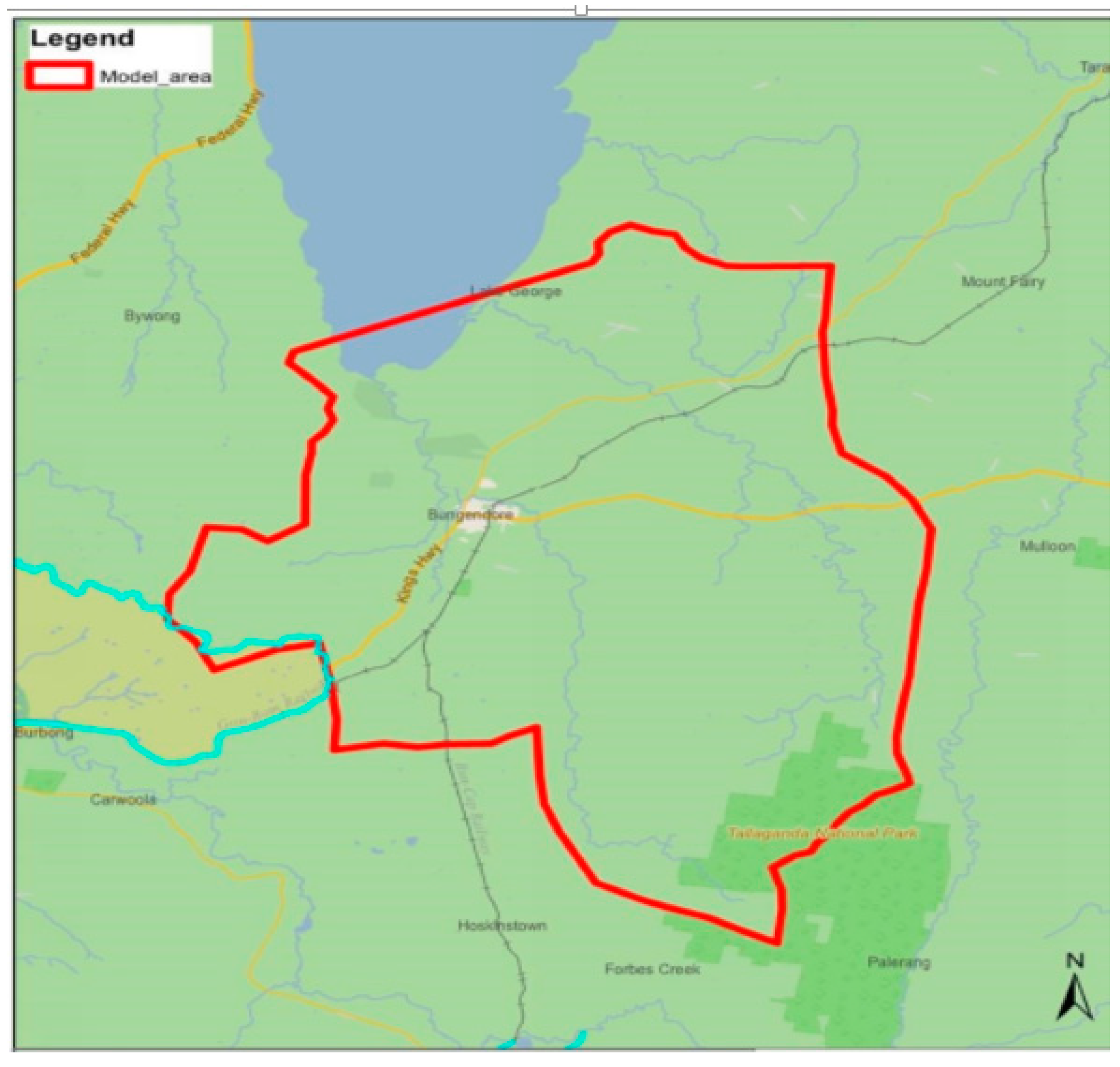
The site (Figure 1) and associated activities are of a sensitive nature and have been described in a generic sense in order for this case study to be published. The main surface water drainages in the study area are Aiga and Soloda Creeks. The project area is dominated by the lake basin to the north and associated channels and alluvial flats bounded by a clearly defined ridgeline to the west and undulating hills to the east and southeast. The elevation varies from approximately 1300 m Mean Above Sea Level (m a.s.l.) at the south-east boundary to a minimum elevation of around 665 m m a.s.l. at the model’s southern-most extent at the outlet of Aiga Creek to the lake.

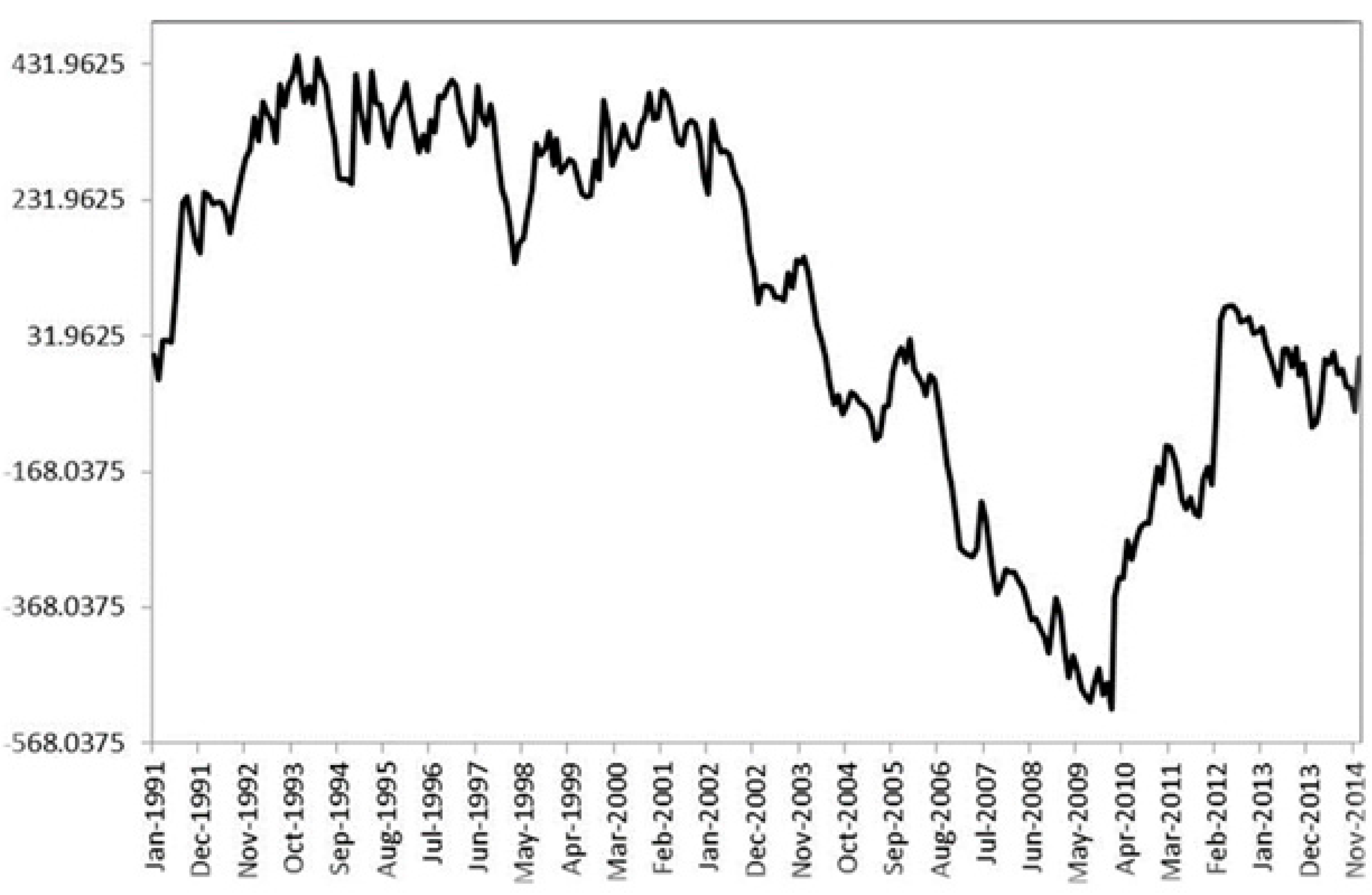
Historical daily rainfall and evapotranspiration data was obtained from the Bureau of Meteorology for the Study area region. Rainfall data was obtained from the study area’s post office station for January 1991 to December 2014. The average annual rainfall and evapotranspiration are 623 mm and 1542 mm, respectively. Long-term rainfall trends for the study area, plotted as cumulative residual rainfall curves (cumulative deviation from monthly average rainfall) show distinct phases (Figure 2), including a pre—2009 (a prolonged period of below average rainfall from 2001 to 2009) below average or drought-dominated period (downward slope), a 1991–1993 period with wetter than average conditions, and a post—2009 period of below average rainfall (upward slope). Cumulative residual rainfall data shows that the rainfall started to recover from the end of the drought period from 2009 up until 2012 but with less q defined trend post 2012 to the present, similar to 1993–1996 (Figure 2). These trends are also captured in long-term stream flow records in the Murray-Darling.

The study area is located in the lake structural basin, having its landform development dominated by ‘sagging’ along a half-graben associated with the Lake Fault. The basement rocks beneath the approximate 80 m thick lake alluvial sequence are dominated by metasedimentary rocks.

3. Methodology

3.1. Water Balance

The task involved water balance modeling of the groundwater system to estimate the likely safe yield of the aquifers. In any aquifer system, a water balance must exist. This balance is expressed very simply by the following equation (Equation (1): [12]):

Recharge + Groundwater inflow = Draft + Groundwater outflow ± change in storage

(1)

The recharge includes such items as natural recharge from rainfall or stream flow and excess irrigation. The Draft includes evapotranspiration; withdrawals for irrigation, industry, and town water supplies; and stock and domestic uses. The change in storage (∆V) (Equation (2)) is expressed as:

$$∆\mathrm{V} = \mathrm{A} \times \mathrm{S} \times ∆\mathrm{h}$$

(2)

where A is the surface area of the water table, S is the storage coefficient or specific yield, and ∆h is the change in water level during the period of analysis.

3.2. Groundwater through Flow

The groundwater flow in any section of aquifer is obtained by using transmissivity, the hydraulic gradient, and the area through which the water is moving. The groundwater flow through an aquifer is obtained from (Equation (3)):

$$\mathrm{Q} = \mathrm{T} \times \mathrm{i} \times \mathrm{W}$$

(3)

where Q is the total groundwater flow through the section considered, T is the average transmissivity in that section, i is the hydraulic gradient (the slope of the potentiometric surface), and W is the width of the section being considered

The methodology employed in this study was built in a spreadsheet model. The errors have been trailed/calibrated to match the residual volumetric fluxes minima (using SOLVER within Excel ^MT environment). SOLVER is used as an add-in tool. It is based on what if analysis to optimize a function value based on constraints. It has three types of cells, namely, target cell, changing cells, and constraint cells. The changing cells must feed into the target cell. The procedure involves setting a target cell, which has a formula with three choices to either maximize or minimize a value or set a specific value. Constraint cells establish constraints for SOLVER.

3.3. Hydrograph Analysis: Rainfall and Time Trends (HARTT)

Time series analysis (transient groundwater hydrograph analysis) with climatic analysis was carried out using a HARTT model [13]. This model, developed by [14], uses a statistical technique for the estimation of trends in groundwater levels. The approach separates the effect of atypical rainfall events from the underlying time trend, and the lag between rainfall and its impact on groundwater is explicitly represented. Rainfall is represented as an accumulation of deviations from average rainfall.

3.4. Surface-Groundwater Interaction Analysis (Base Flow Index)

The Base Flow Index (BFI) program was developed to make the base-flow separation process less tedious and more objective. The program implements a deterministic procedure proposed in 1980 by the British Institute of Hydrology. The method combines a local minimums approach with a recession slope test, estimates the annual base-flow volume of unregulated rivers and streams, and computes an annual base-flow index (BFI, the ratio of base flow to total flow volume for a given year) for multiple years of data at one or more gage sites. Although the method may not yield the true base flow as might be determined by a more sophisticated analysis, the index has been found to be consistent and indicative of base flow and thus may be useful for analysis of long term base-flow trends.

4. Data

Data collection comprised the geological, hydrological, and hydrogeological data sets necessary to characterize the groundwater of the basin. Existing figures and maps related to hydrology and hydrogeology were georeferenced and overlain to analyze and interpret the recharge zone, model area, and sub-surface geology/aquifer configuration. Area and topographic gradients were computed with in the GIS environment (Global Mapper software, version 14, developed by Blue Marble Geographics, Hallowell, ME, USA). Groundwater level time series data from observation bores were analyzed using a statistical method (HARTT: [14]).

4.1. Development of the Conceptual Water Balance Model

The recharge and discharge are the inputs and outputs from a groundwater system. Both quantities are important in understanding how a particular groundwater system functions [15]. A water balance was computed for a hypothetical regional catchment of 180 km² to provide an understanding of the recharge and discharge mechanisms for the area. The boundaries of the area are defined by the surface water catchments, which are generally no flow boundaries. Based on the data assessment and review, at the catchment scale, a potentiometric map suggests that the groundwater level closely follows the topography and that groundwater flow paths are towards the drainage lines.

Monitoring bores in the study area indicated a falling groundwater level since 2001. Although annual drawdown in the deep alluvium has increased relative to the shallow alluvium, recovery levels appear stable. Declining groundwater levels appear to coincide with groundwater pumping and below average rainfall. Under natural conditions, groundwater systems in the study area are primarily recharged by rainfall and creek leakage. Groundwater systems respond to changes in the water balance by the hydraulic transmission of pressure changes (which can be very rapid) and to the physical flow of water from areas of high to low hydraulic head. The time needed by a groundwater system to adapt to a new hydrologic equilibrium depends primarily on its storage size, length, and hydraulic conductivity.

4.2. Recharge

Aquifer recharge in the study area may occur by infiltration of rainwater through soil, leakage of irrigation water through soils, or leakage from urban infrastructure. There is limited opportunity for induced recharge due to groundwater pumping in the area. In this study, 5% and 1.6% rainfall recharge are estimated at the alluvial aquifer (19.8 km²) and fractured rock (159.2 km²), respectively. The percentage of rainfall recharge (5%) for the alluvial aquifer was set based on a sustainability factor, which is the percentage of the recharge volume available for extraction after mitigation is considered.

Recharge is often the most difficult term to evaluate in the hydrological cycle. Identifying recharge sources is a site-specific issue. Basically, it requires understanding of the system. Water balances and numerical models can help in disregarding potential sources or accounting for new ones. In any case, a preliminary conceptual model is needed to get preliminary values of the overall groundwater balance. There is a broad variety of methods to estimate groundwater recharge, but tools to assess the reliability of particular methods are not available. Among the methods commonly used, water table fluctuation, numerical groundwater modelling, Darcy flow calculation, and the water budget method are usually applied to both point and diffuse recharge dominant groundwater basins. The reliability of these methods depends primarily on the quality of data and spatial coverage of the basin. Once the reliability level is known, water resources planners and managers assess the level of risk to aquifers, the environment, and the socio-economic development required for sustainable management of groundwater. Since identifying the recharge area in a catchment is site specific and is very difficult, some methods exist involving stable isotope techniques and artificial tracers [16,17,18].

For the study area, a range of recharge estimates based on the fraction of rainfall were suggested. Early studies estimated that 8% of the rain generates runoff, and most of it ends up recharging groundwater; recent works estimated that 1% of the rainfall is recharge. This has a correlation effect with the calibrated hydraulic parameters carried out. For the model area (179 km²), recharge rates of 0.4% to 2% of effective rainfall were applied based on surface slope, and land usage was considered to assess sensitivity to spatial changes. Subsequently, the 2006 model recharge rates were applied based on landscape units to assess sensitivity to spatial changes. However the total model area was reduced to 165 km²; a recent study estimated 1811 × 10⁶ L/year for the whole study area alluvial groundwater source (59.84 km²) based on 5% rainfall recharge. The portion of the alluvial aquifer that falls within the river catchment (19.8 km²) equates to 494 × 10⁶ L/year, based on the infiltration rate of 5%. A general method of re-assessing recharge is to look at the hydraulic gradient across the model area (River catchment). This includes fractures rock and alluvium.

4.3. Through Flow

There is no flow into the basin because the catchment boundaries are considered to be groundwater divides, which are not flow boundaries. Outflow to the north is through a section of approximately 4.2 km². The through flow is estimated using the optimized hydraulic conductivity (3.5 m/day) and the saturated aquifer thickness (100 m), based on a hydrogeological cross section showing the thickness of the alluvial aquifer (associated with the effect of the Lake Fault). Beneath the lake, drilling has revealed the existence of more than 150 m of fluvio-lacustrine sediments. Also recent studies quoted that the study area alluvial groundwater source is a small palaeo valley with tertiary deposits to a maximum thickness of about 80 m. Fractured rocks were reported with high yields from bores in the area. In addition, the finite available water in alluvial aquifers indicated that inflow from fractured rock aquifers occurs in response to groundwater pumping from the alluvial aquifer. The drainage style of the basin in the more elevated and lower parts of the catchment (which are captured by fracture systems in the bed rock) are, in turn, considered to be in direct communication with alluvial aquifers known to exist in the sub-surface. Large permeable fractures act as primary conduits between deeper and shallower groundwater systems. The effects of weathering are usually limited to depths of 100 m. Below these depths, fractures tend to be closed by the weight of the overlying rock. Therefore, the permeability of these groundwater systems generally decreases with depth. However, water-yielding zones have been found at depths of several hundred meters. There is insufficient information to assess the component of deep circulation and hence the deep groundwater resource within the fractured rock systems. However, the hydrographs from monitoring bores screened in the alluvium and fractured rock responded identically to the differences in rainfall over a period of time (greater than 10 years). Therefore, considering the top layer of the fractured aquifer, the current saturated aquifer thickness (100 m) seems justifiable; the cross sectional flow width out of the river catchment is 4.2 km; hydraulic gradient along the inflow path is 0.003, derived from the potentiometric map; and the outflow volume for the river catchment is ~1589 × 10⁶ L/year.

Analytical calculations to estimate outflow confirm that a modelled boundary outflow volume of about ~1300 m³/day (475 × 10⁶ L/year) is reasonable, but this could be substantially higher or lower. Using Darcy’s law (Equation (2)), a flux of about this magnitude would be expected based on an aquifer thickness of 33 m, aquifer width of 4.2 km, average hydraulic conductivity of 3.46 m/day, and a horizontal hydraulic gradient of about ~0.003 across a relatively flat plain. The modelled water table gradient in this area was estimated as 0.003, compared to 0.0023 estimated from the map provided by previous works, based on water levels in a limited number of bores with unknown screen depths. Actual boundary outflow rates cannot be determined without nested groundwater bores in this area to determine stratigraphy, local hydraulic gradients, and other measures of groundwater flow. In the current study, all the estimated parameters match the estimate carried out by previous works, except the saturated aquifer thickness (assumed 100 m instead of 33 m). The saturated aquifer thickness estimated by previous works was 33 m. However, the current study has assumed 100 m, based on the review of the reports, specifically a hydrogeological cross section, whereby the location of the cross section line/transvers is very close to the through flow model area shown in previous works. The topographic gradient is ~0.02, and the groundwater hydraulic gradient is 0.003. This indicates that the site is either very low recharge and/or moderate permeability.

In line with this, a noble approach has been followed to assess and constrain the discharge coming out of the model area to sustain the lake level using the whole lake catchment (932 km²) and lake water balance analysis (which is 16% of the total catchment). The maximum influx (outflow from the model domain) to sustain the historic lake level was estimated using Darcy’s law (cross section through flow) and further constrained in a regional context using lake catchment (including River, Soloda Creek, and Guragure Creek) and lake water balance analysis. Based on the analysis, the current model area, which comprises River and Soloda Creek contributes 40% of the lake catchment. Based on the lake water balance, there is a deficit between input and output computation, and hence there should be a groundwater input to sustain the historical lake area. The average annual precipitation and evaporation areas are 623 mm and 1542 mm respectively, and the pan evaporation factor is 0.7. Annual runoff is assumed to be 8% of the precipitation. Eventually, the portion of the groundwater inflow feeding the lake was computed. This is one of the means to constrain the discharge, which adds more confidence to the recharge estimation. This is very important because the size of a sustainable groundwater development usually depends on how much of the discharge from the system can be captured by the development. Capture is independent of the recharge. Instead, it depends on the dynamic response of the aquifer system to the development using the numerical model. The idea that knowing the recharge is important in determining the size of a sustainable groundwater development is a myth. This idea has no basis, in fact. The important entity in determining how a groundwater system reaches a new equilibrium is capture. How capture occurs in an aquifer system is a dynamic process [19,20]. Following this study, lake water balance assessment was indirectly considered as prior information for the numerical model calibration of the discharge from the model area using a conductance parameter. Conductance is a key parameter to estimate the discharge volume together with the change in the simulated hydraulic head between time steps.

4.4. Groundwater Abstraction

The total estimated abstraction is 700 × 10⁶ L/year, from six bore licenses. This volume may increase as existing non-volumetric licenses/applications submitted during amnesty periods/current aquifer interference activities have volume allocations resolved. The majority of the groundwater abstraction is associated with alluvial aquifers that have significant storage, unlike the adjacent catchments (such as the Rama, Mihtsaeb-Hizaetie Creek, and fractured rock sub-catchments in the Mereb-Leke region), which are associated exclusively with fractured rock aquifers.

Evapotranspiration was assumed to be nil due to the relatively deep water table.

5. Results and Analysis

The base flow of the streams generally corresponds to the volume of water that recharges the shallow groundwater system and re-emerges as springs and seeps to feed the streams during the dry season. There is no true dry season in the surroundings of the study area; rainfall continues year round. Nevertheless, the stream flows during May and June are assumed to approximate groundwater contribution because rainfall in those relatively dry months, at about 2.86 mm/day (averaged from three nearby stations), is nearly all consumed by evapotranspiration of 2.50 mm/day (Monteith-Penman calculation). In order to convert the base flows to recharge rates, the area-normalized flows (m³/s/km²) in

Table 1. Annual Flow, Base Flow, and Runoff in the surrounding Streams.

	Suluh River Drainage—South			Eastward Flow	Medimar River Drainage—North
	Zarema	Mai-Nigus	Mai-Guagua	Mai-Sessela	Giba	Shebele	Dawa
Area (km2)	5.7	0.8	1.75	8.45	7.0	4.85	0.75
	(m3/s)
June Flow	0.29	0.04	0.09	0.43	0.36	0.25	0.04
Annual Average	0.574	0.079	0.178	0.853	0.705	0.489	0.078
Area Normalized Flow	(m3/s/km2)							Average
	0.051	0.050	0.051	0.051	0.051	0.052	0.053	0.051
	(mm/year)
Base Flow (May)	1604	1577	1622	1605	1622	1626	1682	1620
Annual Total	3177	3121	3214	3182	3176	3181	3259	3187
Runoff	1572	1544	1592	1577	1554	1555	1577	1567

were converted to mm/year. Table 1 shows that, in the vicinity of the study area, shallow recharge and discharge occurs at the approximate rate of 1620 mm/year. Total streamflow represents about 3187 mm/year (also by dividing flow rates by areas), so that runoff during the wetter months averages about 1567 mm/year. The climate region of the surrounding streams exceeds three times that of the study area.

Comparison of the baseflow at the surrounding of the study area with nearby rivers is given in

Table 2. Comparison of Base Flows of Nearby Rivers.

	Drainage	Average Base	Area Normalized	Base Flow
	Area	Flow	Flow	Month
	(Km2)	(m3/s)	(m3/s/km2)
Study area vicinity Streams	29.3	1.58	0.051	June
Medimar River	101.0	5.44	0.053	May
Mereb River	41.1	2.32	0.056	May

.

Runoff and base-flow values, along with precipitation and evapotranspiration numbers can also be used to roughly estimate how much of the annual precipitation percolates through the cover sequence to recharge the basement aquifer below. Table 1 shows three attempts to quantify the water balance:

Deep Recharge = Precipitation − Runoff − Base Flow − Evapotranspiration

Evapotranspiration is assumed to be 912 mm/year, as calculated using the Penman-Monteith method (this may be the least constrained number in the calculation). Base flow and runoff in each case are the values shown in Table 1. The three cases vary only in the amount of recharge applied. In

Table 3. Calculated Base Flow (Shallow Recharge), Runoff, and Deep Recharge. (A) Original Calculations using Guna precipitation; (B) Calculations using Medimar Station precipitation; (C) Calculations using average precipitation from three stations.

A
Yearly Precipitation	(mm/Year)	4866
Base Flow	1620	33.3%
Evapotranspiration	912	27.1%
Runoff	1567	32.2%
Deep Recharge	(remainder)	7.4%
B
Yearly Precipitation	(mm/Year)	3701
Base Flow	1620	43.8%
Evapotranspiration	912	24.6%
Runoff	1567	42.3%
Deep Recharge	(remainder)	−10.8%
C
Yearly Precipitation	(mm/Year)	4053
Base Flow	1620	40.0%
Evapotranspiration	912	22.5%
Runoff	1567	38.7%
Deep Recharge	(remainder)	−1.1%

A, a high value of 4866 mm/year, from Guna records, results in a deep-recharge value of 7.4 percent of precipitation (360 mm/year). Such a high rate of recharge to the basement system is not supported by pumping-test data. In Table 3B, a low precipitation rate of 3701 mm/year, from the Medimar Station, results in a deep-recharge deficit of −10.8%. That is, evapotranspiration and stream flows together exceed precipitation by about 399 mm/year. In Table 3C, an intermediate value of precipitation, 4053 mm/year, is derived by averaging the yearly values from the Guna, Medimar, and Tekeze weather stations. This value results in a very small deficit of just 1.1 percent, or about 44 mm/year. The smaller numbers are much more consistent with recent model calibrations to long-term pumping, which show less than 1% recharge to the deep groundwater system (the negative value illustrates the high-degree of uncertainty in these calculations).

5.1. Surface Water—Groundwater Interaction

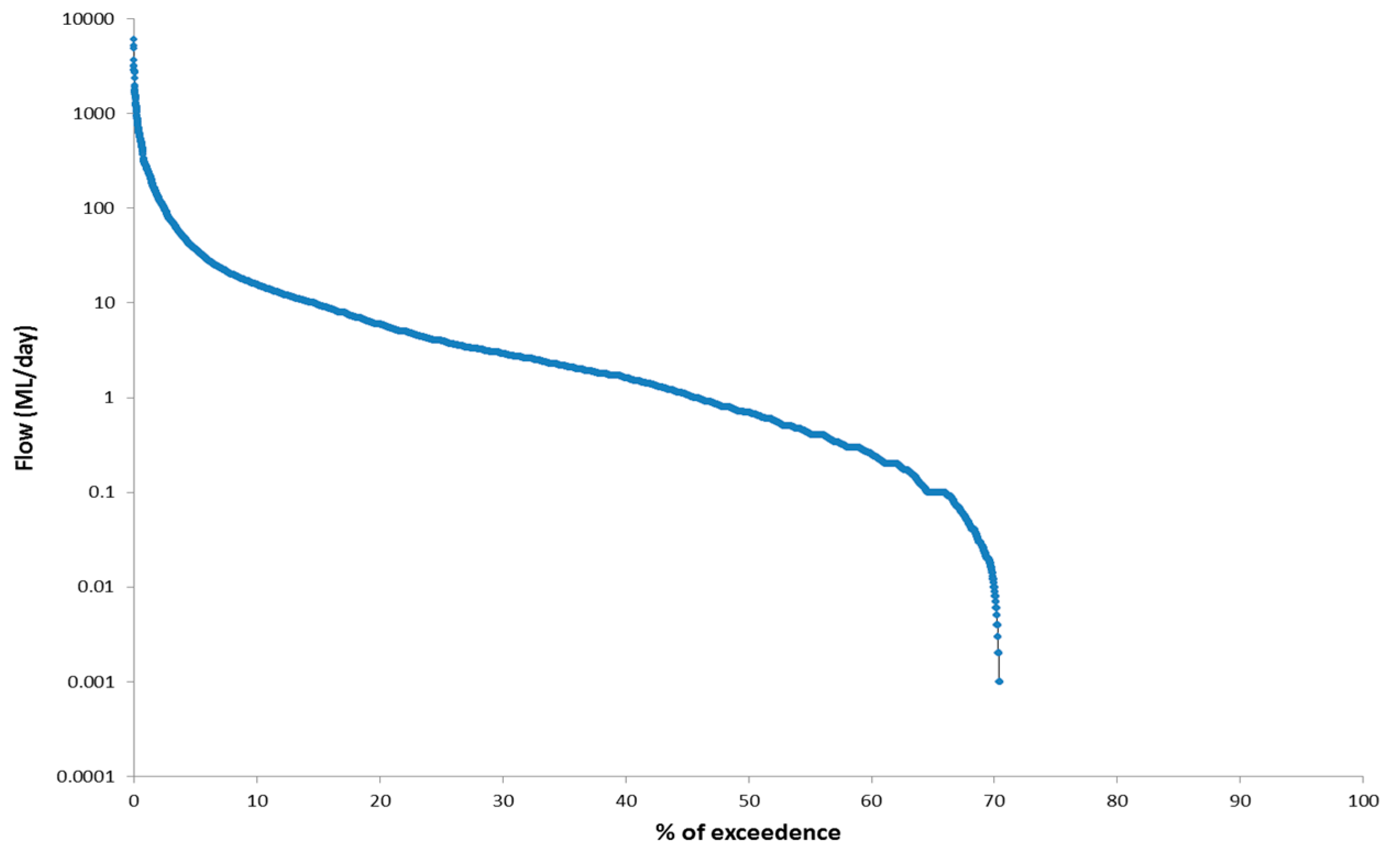
In the study area, stream flow leakage or base flow is assumed to be minimal or nil, unlike the surrounding streams. There is no data available to confirm whether the stream is recharging or discharging groundwater. Baseflow stream gauging is required to assess this. The drainage style of the basin is characterized by a medium density of ephemeral streams located in the more elevated parts of the catchment. In the lower parts of the catchment, the more ‘mature’ drainage is captured by fracture systems in the bedrock, which, in turn, are considered to be in direct communication with medium to coarse alluvial aquifers known to exist in the sub-surface. Soloda Creek flow recorded at Soloda was analyzed using the frequency analysis method to estimate the degree of surface water/groundwater interaction. Frequency analysis characterizes baseflow using a Flow Duration Curve (FDC) by deriving the relationship between the magnitude and frequency of stream flow discharges from the hydrographic record.

The FDC provides information on the baseflow component of stream flow. The median flow (Q50) is the discharge that is equalled or exceeded 50% of the time. The part of the curve with flows below the median flow represents low-flow conditions. Baseflow is interpreted to be significant if this part of the curve has a low slope, as this reflects continuous discharge to the stream. A steep slope for these low-flows (e.g., Figure 3) suggests very small/nill contributions from natural storages like groundwater. Various indices are used to represent the characteristics of the low-flow regime for a stream. The ratio of the discharge that is equaled or exceeded 90% of the time to that of 50% of the time (Q90/Q50) is commonly used to indicate the proportion of stream flow contributed from groundwater baseflow [21].

The baseflow index (Q90/Q50) for Soloda Creek at Soloda is estimated to be 0.001, indicating that there is a loose/nil connection between surface water and groundwater (i.e., very low baseflow stream), and hence, in the long term, abstraction activities would be expected to have a minor impact on the surface water flow. The river has no gauged data but shares the same geology, landuse, slope, and climate with the adjoining sub basin (Soloda Creek). It is assumed that both creeks share similar surface water-groundwater connectivity. The other output components including through flow, abstraction, and evaporation were estimated using the available data set.

5.2. Groundwater Dynamics and Long Term Evaluation

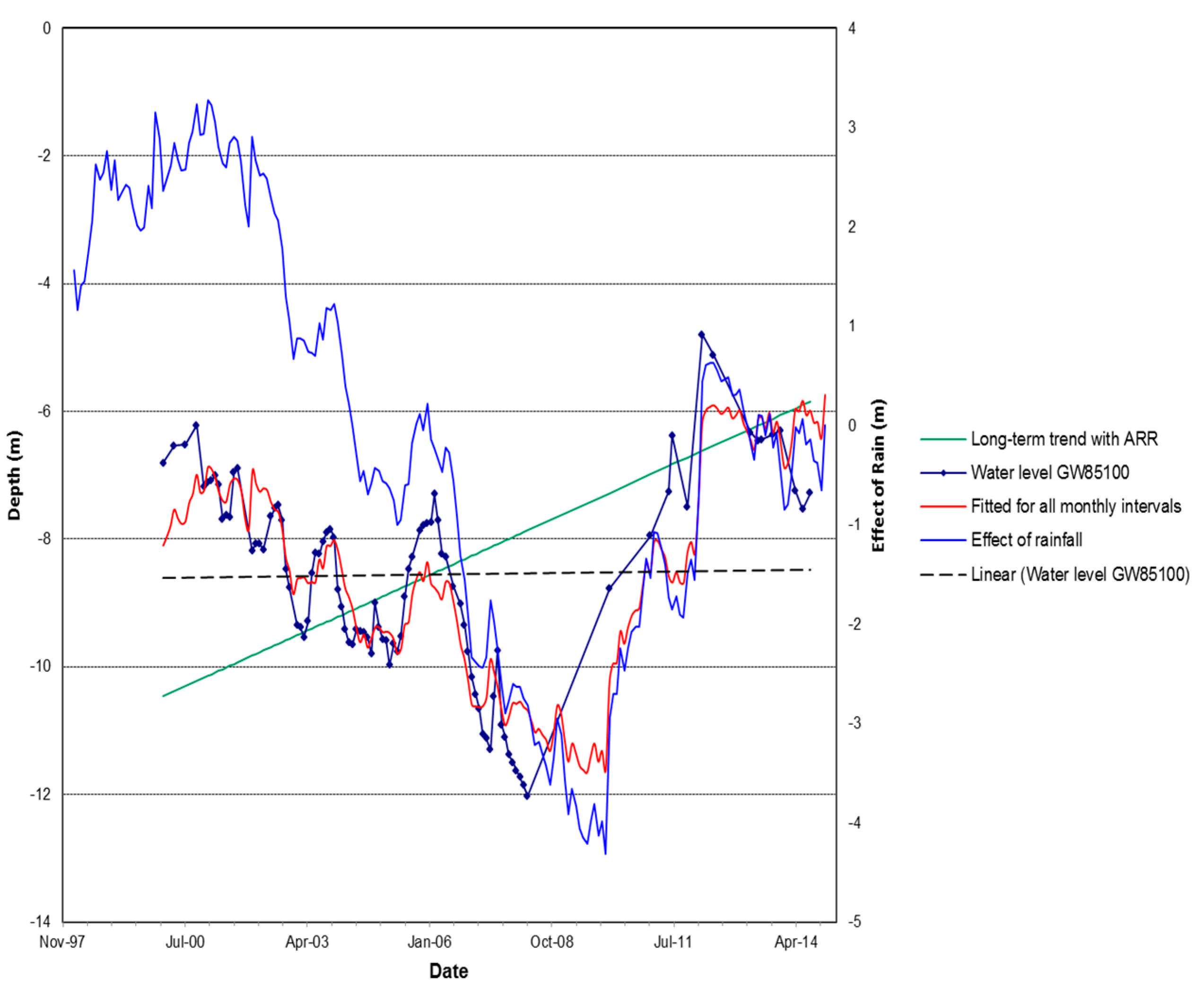
The hydraulic and chemical characteristics of the unconsolidated sedimentary groundwater systems are highly variable depending on environment of deposition and their location in the landscape. Some thick riverine plain sequences composed of sandy gravels have very high primary porosity, permeability, and yield characteristics. In valleys and riverine plains, the fold belt and tertiary volcanic fractured-rock systems may be overlain by unconsolidated sediments of variable thicknesses. At these locations, the unconsolidated sediments generally control shallow groundwater characteristics and responses. Monitoring bores in the study area indicated a falling groundwater level since 2001. Although annual drawdown in the deep alluvium has increased, relative to the shallow alluvium, recover levels appear stable. Declining groundwater levels, in one of the well fields, appear to coincide with groundwater pumping and below average rainfall (Figure 4).

The time series modelling (Hydrograph Analysis: Rainfall and Time Trend: HARTT; [13,14,22] was employed to decompose the groundwater hydrograph into individual drivers, mainly the climatic influence. To analyse the hydrograph, it requires enough-long-term rainfall data for the delay period and for the long term analysis. For the representative observed bore, shown for a 14 year monitoring period, the model predicts that 77% (R² for the regression) of the hydraulic head observation in bore hydrograph GW85100 can be explained by climatic/rainfall, with no significant lag time (0 month delay/best-fit delay: Figure 4). The rest (23%) can be attributed to human influence, mainly due to the nearby pumping/bore field for town water supply, as this is the case for the monitoring well (GW85100) analyzed. The underlying time trend rate (long-term trend with Average Residual Rainfall (ARR); Figure 4), is estimated to be 2.21 mm/year (i.e., related to groundwater system/storage).

5.3. Water Balance

A water balance was computed for a regional catchment of 373.6 km² to provide an understanding of the recharge and discharge mechanisms for the area (Figure 5). The boundaries of the area are defined by the surface water catchments, which are generally no flow boundaries.

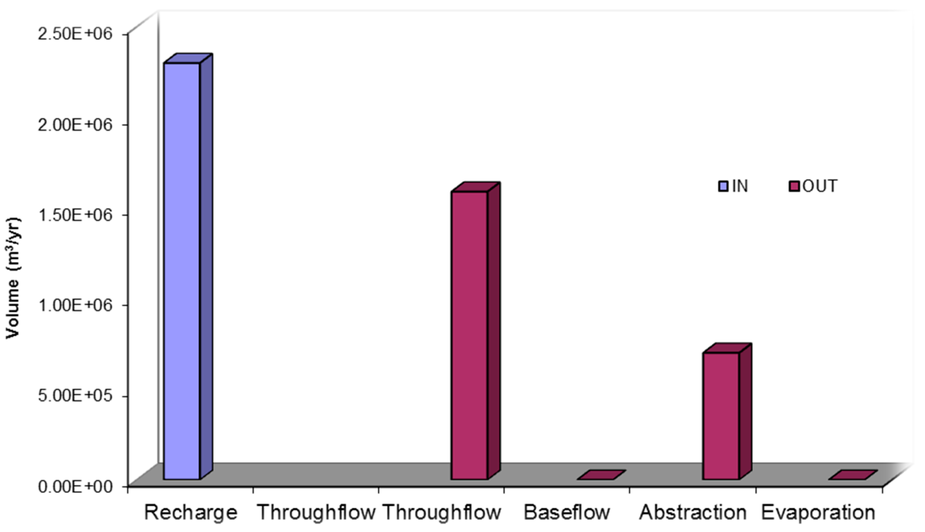
The error in the water balance is about 0.43%. As shown in

Table 4. The water balance components.

Inputs	Input (106 L/Year)	Output (106 L/Year)
Rainfall Recharge areal	2299	0
Upland recharge
Groundwater inflow from adjacent basins
Irrigation return flow
Through flow to the/out of the catchment	0	1589
Baseflow		0
Groundwater Abstraction		700
Evapotranspiration		0

, recharge into the groundwater system discharges mainly via through flow towards the lake, with abstraction from existing wells. The water budget reveals that the through flow component is quite insignificant.

Under natural conditions, groundwater systems in the study area are primarily recharged by rainfall and creek leakage (if any). Groundwater systems respond to changes in the water balance by hydraulic transmission of pressure changes, which can be very rapid, and as physical flow of water from areas of high to low hydraulic head. The time needed by a groundwater system to adapt to a new hydrologic equilibrium depends primarily on its storage size, length, and hydraulic conductivity. The error attributed to change in storage volume is assumed to be minimal. The analytical estimate of change in storage volume is about 6.5 × 10⁶ L/year (<0.001% of the recharge volume). The storage volume change was computed based on values of 0.2 and 0.00015 for the specific yield and storage coefficient of the alluvium aquifer and fractured rock, respectively; change in groundwater level fluctuation was on average 1.5 m and 2.5 m for the alluvium aquifer and fractured rock, respectively; and areas of 19.84 km² and 159.2 km² were determined for the alluvium aquifer and fractured rock, respectively. The water balance model was constrained using a data set from the salinity of the groundwater and surface water and surface water flow data and time series groundwater heads (hydrographs).

6. Sensitivity Analysis

A sensitivity analysis was carried out to determine which variables of the model are more sensitive and to estimate the variation in output parameters that could arise due to uncertainties in the sensitive variables. The objective of sensitive analysis was to evaluate the impact of changing input parameters on the water balance in the model [23,24]. It was also performed to determine if the response of the model to the input variables agrees with the knowledge and hypothesis that led such variables being chosen. The capacity of the model to reproduce the non-linearity of the physical system was also tested. It means that if we increased or decreased the variable by a factor of two, for example, then we could not expect the response to increase or decrease by the same factor.

Starting from the base model, a certain number of changes are performed for each water budget component according to a defined number of intervals and ranges. This technique identifies the most sensitive parameters in the estimation of the water balance and allows a quantitative analysis of how errors are fed through the input parameters.

The output values were analyzed using the following relation in order to evaluate the effect of the perturbation:

$$D(\%)=\frac{Op-Ob}{Ob}\times 100$$

(4)

where Ob represents the base value and Op represents modified parameter. Negative deviations would indicate a decline in groundwater input.

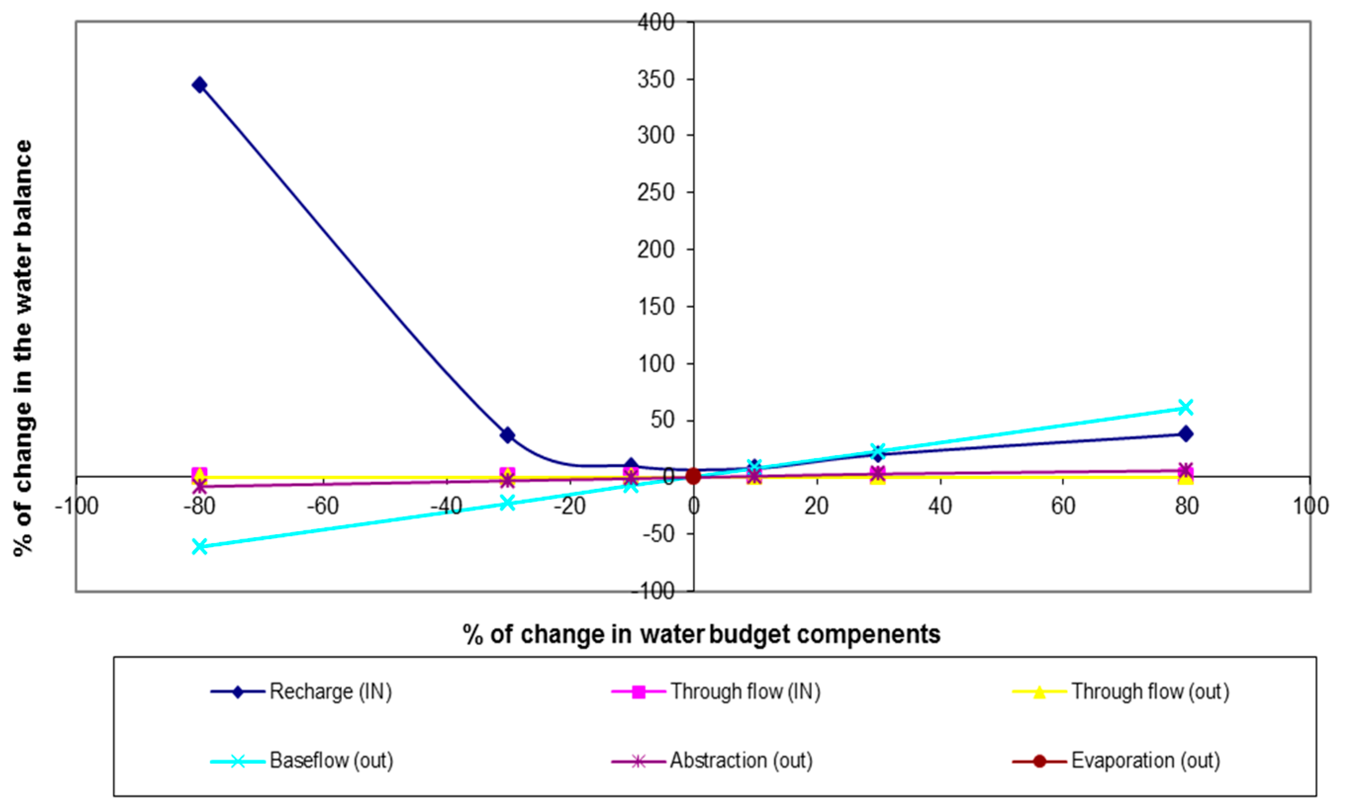
Figure 6 shows that the model is most sensitive to recharge and baseflow. The variables to which the model is least sensitive are through flow (IN/OUT), evaporation, and abstraction. The sensitivity analysis shows that recharge is most sensitive among the other water budget components. Abstraction followed by through flow is a relatively less sensitive component (Figure 6).

7. Discussion

The current study presents the long-term groundwater water balance of a river sub-catchment area. The method provides insight into the process of estimating the hydraulic and recharge parameters within the previous model. Such analysis can be accrued for upland hills, basins, or sub basins, whereby the mass balance is useful for resources, impact, and social, economic, environmental, and ecological aspects development. The current analysis presents on how to analyse the data set before putting forward any further plan for the connectivity of surface-groundwater. The original set up of the model was considered reasonable given the available information at the time. However, the following points should be considered, which likely impact the estimated sustainable yield: the saturated aquifer thickness and the vertical hydraulic conductivity value (Kv) of the modeled aquifers was unrealistic. A vertical hydraulic conductivity distribution of 1 × 10⁻²⁶ m/day has been assigned for the bottom layers of fractured rock, and these need to be re-assessed. The ratio of horizontal hydraulic conductivity (Kh) to vertical hydraulic conductivity (Kh/Kv) is in the order of 10⁻²⁵, which is unusually high, and the recharge estimate is controversial, being correlated with the hydraulic conductivity value.

Based on the current water balance calculations, the long-term average annual extraction limit is ~1610 × 10⁶ L/year (i.e., 70% of recharge generated over the remainder of the aquifer area). A sustainability factor of 70% was calculated via a risk assessment. A recent study indicates the Basic Landholder Rights (BLR) for the area to be approximately 25 × 10⁶ L/year. Therefore the estimated total groundwater entitlement available for licensing is approximately 1585 × 10⁶ L/year. The BLR volume may increase during the term of the plan if there is growth in access to BLR. Water balance modelling indicates that the long-term average annual extraction limit may be higher than that estimated by previous works.

The assessment suggests that current extraction removes water mainly from the through flow component not storage. Therefore there may be room for an expansion of extraction, which accesses storage as well. Storage is mainly within the alluvial system but may also include the much larger but much lower storage fractured rock system. It is recommended to intercept the through flow water before it reaches the lake, as water entering the lake system becomes more saline due to evapotranspiration and deep circulation processes, effectively sterilising the water. The data analysis and conceptual water balance modelling indicates that the groundwater system may not be under stress. It is estimated that an additional capacity of groundwater may be allocated.

7.1. Perennial Sustainable Yield

A groundwater reservoir may be defined as the maximum amount of groundwater that can be salvaged each year over the long term without depleting the groundwater reservoir. The perennial yield is ultimately limited to the maximum amount of the natural discharge that can be salvaged for beneficial use [25,26,27]. Based on the groundwater balance analysis, the through flow estimated is about 1589 × 10⁶ L/year. Water management problems are likely to increase, even in areas of net positive water balancem due to increased climatic variability, increased demand (irrigation and domestic use), and double amplification within water catchment systems, whereby runoff tends to amplify changes in rainfall and reservoir schemes will tend to amplify changes in mean annual rainfall in the projected scenarios. Further, increased winter precipitation may not be of much use because, without increasing storage, it will tend simply to increase spillage losses.

7.2. Impacts

Water sources are defined as ‘highly connected’ if 70% or more of groundwater pumped in an irrigation season is derived from stream flow. Depletion of groundwater can pose a risk to groundwater dependent ecosystems (GDEs) from declining groundwater levels, beneficial use of the groundwater, and structural damage of the aquifer. Socio-economic risks can be overall community dependence on groundwater extraction, relative importance of groundwater supply (due to lack of alternative water sources), economic significance of the groundwater source for irrigation or industrial activities, and the level of local employment associated with the commercial uses of groundwater. Strategies to manage risks and therefore ensure groundwater extraction are sustainable. To mitigate the effects of the medium risk to the aquifer in relation to water quality and beneficial use of the groundwater, irrigation pumping scheduling is being imposed on the water source. This has resulted in the overall reduction of the aquifer risk from medium to low.

Investing in groundwater monitoring and hydrogeological investigations can greatly reduce the uncertainty in groundwater yield estimates. Irrigators who have recorded groundwater and water salinity data regularly for several decades have very valuable information on which to base farming decisions. There are many strategies to reduce yield uncertainty that are not yet practised widely in Australia. Automated monitoring of groundwater levels with real-time reporting on the internet is already in place for some aquifers in the US and New Zealand. In Israel, it is mandatory that all new bores are logged with downhole geophysical sondes, subjected to standard bore pump tests, and tested for a range of water quality parameters.

7.3. Limits to the Availability of Water

The long-term average annual extraction limit (LTAAEL) has been set at 70% of the estimated rainfall recharge into the aquifer (1268 × 10⁶ L/year). The percentage of recharge set was based on a sustainability factor described above. The accepted method for setting an extraction limit for all inland alluvial groundwater systems is to base the LTAAEL on a history of extraction. Where there is little available information on the history of extraction, a proportion of entitlement is used in a similar metered system as the basis for usage. The study area alluvial groundwater source has limited usage data and is a unique system, so it could not be compared to a similar system to estimate the history of use. Therefore the sustainability factor approach was adopted. The risk associated with using this approach was considered to be low as the total licensed entitlement (1218 × 10⁶ L/year) is less than the LTAAEL set using the sustainability factor approach (1268 × 10⁶ L/year). The average annual extraction against the long-term average annual extraction limit (LTAAEL) was assessed. Extractions are assessed on an annual basis against the LTAAEL. This assessment is based on the long-term sustainability of the aquifer. The analysis suggests that it is appropriate to use a three-year rolling average to measure Potential Growth in Use (GIU); GIU should be deemed to occur if the three-year rolling average use exceeds the LTAAEL by 5% or more. This means that rather than apply the response immediately upon determining that extractions have exceeded the LTAAEL, a margin of 5% is permitted before a GIU response is applied. The time period over which the growth in extraction assessment is made is based on a consideration of seasonal variations in historical usage patterns and accounts for any calculation errors without triggering a GIU response. The response tolerance was designed to accommodate the peaks and troughs of the usage data on which the LTAAEL was founded.

8. Conclusions

The study provides an understanding of the recharge and discharge mechanisms for the area. Recharge has been often the center of focus to estimate yield. However, little attention has been paid to estimate discharge. Estimating discharge gives a better picture of the yield estimate. Also, it helps to double-check the reliability of yield estimate. This reduces uncertainty & flawed safe yield value set by the simulations. In this study, the discharge component was constrained using a noble approach, assuming that the portion of the groundwater feeding the lake basin is the principal outflow from the study area sub-catchment. The water budget analysis can provide insight for the recharge and discharge input and helps to constrain the dynamic model assessment, together with the initial conditions, boundary, hydrostratigraphy, and flow system, which are assumed to be pillars of a comprehensive site conceptual model.

Often conceptual model uncertainty is overlooked. The errors and uncertainty related to a conceptual model can be narrowed down substantially using the method employed in this paper. This study demonstrates the importance of mass balance analysis in relation to (and its implications on) effective and sustainable resource management, as well as improving understanding of climate impacts on groundwater levels.

The current study assists in the assessment of the impact of future climatic variability on the rate of aquifer recharge; long-term abstraction planning in the region; better quantification of the constraints of delivering increased groundwater volumes over the long term, including delineating groundwater targets for additional groundwater supplies (such as locating new bores within fractured rocks/alluvial aquifers and locating new bores within the alluvial channel close to the discharge into lake); and assessment of the level of increased groundwater abstraction at the existing wells. Further to this study, a numerical groundwater model should be established to provide more accurate assessment of the groundwater processes and the water balance and to enable a range of abstraction scenarios at the river sub-catchment to be evaluated.

The findings of the current study (including the water balance output and time series data analysis) can be used as a key input to constrain the future application of a numerical model, cross-check the reliability of the numerical water balance output with the conceptual water balance figures (i.e., to confirm the capacity of the current estimated yield); to suggest that groundwater storage does contribute to planned abstraction, apart from the through flow; and to assess the impacts of additional groundwater abstraction on the aquifers.