Estimating the Sediment Flux and Budget for a Data Limited Rift Valley Lake in Ethiopia


1
School of Civil and Environmental Engineering, Addis Ababa Institute of Technology (AAiT), Addis Ababa 1000, Ethiopia
2
Department of Earth and Environment, Florida International University, Miami, FL 33199, USA
*
Author to whom correspondence should be addressed.
Hydrology 2019, 6(1), 1; https://doi.org/10.3390/hydrology6010001
Submission received: 15 October 2018
/
Revised: 4 December 2018
/
Accepted: 9 December 2018
/
Published: 23 December 2018
(This article belongs to the Special Issue Catchments Hydrology and Sediment Dynamics: Concepts, Measuring and Modelling)
Abstract
:Information on sediment concentration in rivers is important for the design and management of reservoirs. In this paper, river sediment flux and siltation rate of a rift valley lake basin (Lake Ziway, Ethiopia) was modeled using suspended sediment concentration (SSC) samples from four rivers and lake outlet stations. Both linear and non-linear least squares log–log regression methods were used to develop the model. The best-fit model was tested and evaluated qualitatively by time-series plots, quantitatively by using watershed model evaluation statistics, and validated by calculating the prediction error. The contribution of the ungauged basin was estimated by developing a model that included the terrain attributes and measured sediment yield (SY). The bedload of the rivers was estimated and the total amount of sediment transposed into the lake was calculated as 2.081 Mton/year. Annually, 0.178 Mton/year of sediment is deposited in floodplains with a sediment trapping rate of 20.6%, and 41,340 ton/year of sediment leaves the lake through the Bulbula River. As a result, the net sediment deposition rate of the lake was estimated as 2.039 Mton/year and its trapping efficiency was 98%. Accordingly, the lake is losing its volume by 0.106% annually and the half-life of the lake is estimated as 474 years. The results show that the approach used can be replicated at other similar ungauged watersheds. As one of the most important sources of water for irrigation in the country, the results can be used for planning and implementing a lake basin management program targeting upstream soil erosion control.
1. Introduction
Sedimentation caused by catchment erosion is reducing a significant proportion of the original storage capacity of many lakes [1]. Some reports show that reservoirs are losing about 1–2% of their volume annually due to sedimentation. For many lowlands, rivers transport sediment from the catchment to lakes [2] and the benefits, lifespan, and the sustainability of lakes can be controlled by sedimentation [3]. Estimating the sediment loads of lake basins is important to assess lake siltation, identify sediment source areas, plan watershed management programs, and evaluate the effect of sedimentation on water resources [4,5]. Sediment budget estimation of watersheds will require identifying major sediment sources (upland erosion, gulley or channel erosion, riverbank erosion and also river bed contributions) [6].
Tackling sedimentation in water bodies will require a research-based approach to properly understand the processes that govern the sediment detachment, transport, and deposition [7]. For a river basin, the sediment yield can be obtained by calculating from sediment data at gauging stations [8]; analyzing reservoir sedimentation data [9]; estimating using sediment transport equations [6], and/or predicting using models [10,11,12,13,14,15,16,17,18,19,20,21,22,23,24]. There are a number of empirical and non-empirical approaches to quantify sediment yield of watersheds but none of them are believed to be applicable to all watersheds [25,26]. The absence of a robust approach for estimating sediment yield will necessitate the use of modified approaches that take in to account the topography, soils, land cover, watershed management and other factors.
For instance, to obtain the indicator for environmental changes like lake sedimentation, lake ecosystem functioning, and to estimate the life time of reservoirs [27,28,29], the bathymetric surveying method is the most accurate. But, in quantifying both soil erosion and deposition rates, the sediment budgets estimated from repeated bathymetric surveys cannot indicate the actual soil loss rate of the catchment. In the same way, for river basin and reservoir management, using an empirical model is one of the popular means of estimating sediment loads. In predicting soil loss, the most commonly used empirical models are the universal soil loss equation (USLE) [30] and its derivatives. However, in the case of developing countries like Ethiopia, it is believed to be difficult to acquire the complete datasets for these models [31]. Most of the sediment modeling tools were developed for data rich areas making them less applicable in data scarce regions of the world. While field measurement of sediment load is reliable, it is not always feasible since it is expensive and time-consuming. To generate sediment load for areas of limited continuous observation, the use of rating curves is recommended [2]. Today, a rating curve is commonly used by engineers and scientists for various purposes [22]. Sediment rating curves are especially used by engineers and hydrologists to estimate the life expectancy of dams, while scientists use it to study depositional and erosional environments [32]. For example, a rating curve has been applied to the Yangtze River, China, for trend analyses [33]; for sediment rating curve modification of the Marun Dam, Iran [34]; for sediment load estimation in Algeria in the Mellegue River Basin [35], to estimate the Rhône River contribution for Lake Geneva [36]; to assess the sediment concentration rating for the upper Blue Nile [37]; and to revise lake sediment budgets of Lake Tana, Ethiopia [38].
In addition, sediment rating curves have proven to be useful for estimating sediment loads from ungauged watersheds. They are also useful for validating sediment yield models. A number of researchers have used sediment rating curves in the Lake Tana basin [39,40,41] and Lake Ziway [42] to generate observed sediment data in places and periods where there are no field data. This has also been used for calibrating and validating sediment simulations in models like Soil and Water Assessment Tool (SWAT). Studies indicate that the predicted suspended sediment load from sediment rating curve techniques is either underestimating [2,43] or overestimating [44] the sediment load when compared with the corresponding observed sediment load. To compensate for this, some modifications have been applied; these include applying correction factors [45] and using non-linear regression methods [43]. Even though there are different compensation methods employed to develop a sediment rating curve, none of them have received universal acceptance [8]. The predicting quality of a given sediment rating curve will depend on the fitting methods, and a single sediment rating curve cannot be employed for all rivers. Hence, developing a best-fit model is required in order to be accurate in sediment estimation. Reference [46] suggests to develop a best-fit rating curve model to estimate long-term suspended sediment data records for rivers with a limited sediment database.
The Lake Ziway basin is one of the data scarce areas of Ethiopia and the historical measured sediment data is very limited. Moreover, according to Reference [47] there are two proposed dam sites on its tributary rivers for multipurpose use. This necessitates studying sediment accumulation rates and evaluating best management options to increase the life span of the lake by reducing upland soil erosion and lake sedimentation. Hence, the objectives of this study are to (1) develop the best-fit rating curves to estimate suspended sediment loads; (2) calculate the sediment flux rates of the lake tributary rivers; and (3) determine the sediment accumulation rates of the lake.
2. Study Area
2.1. Location and Topography
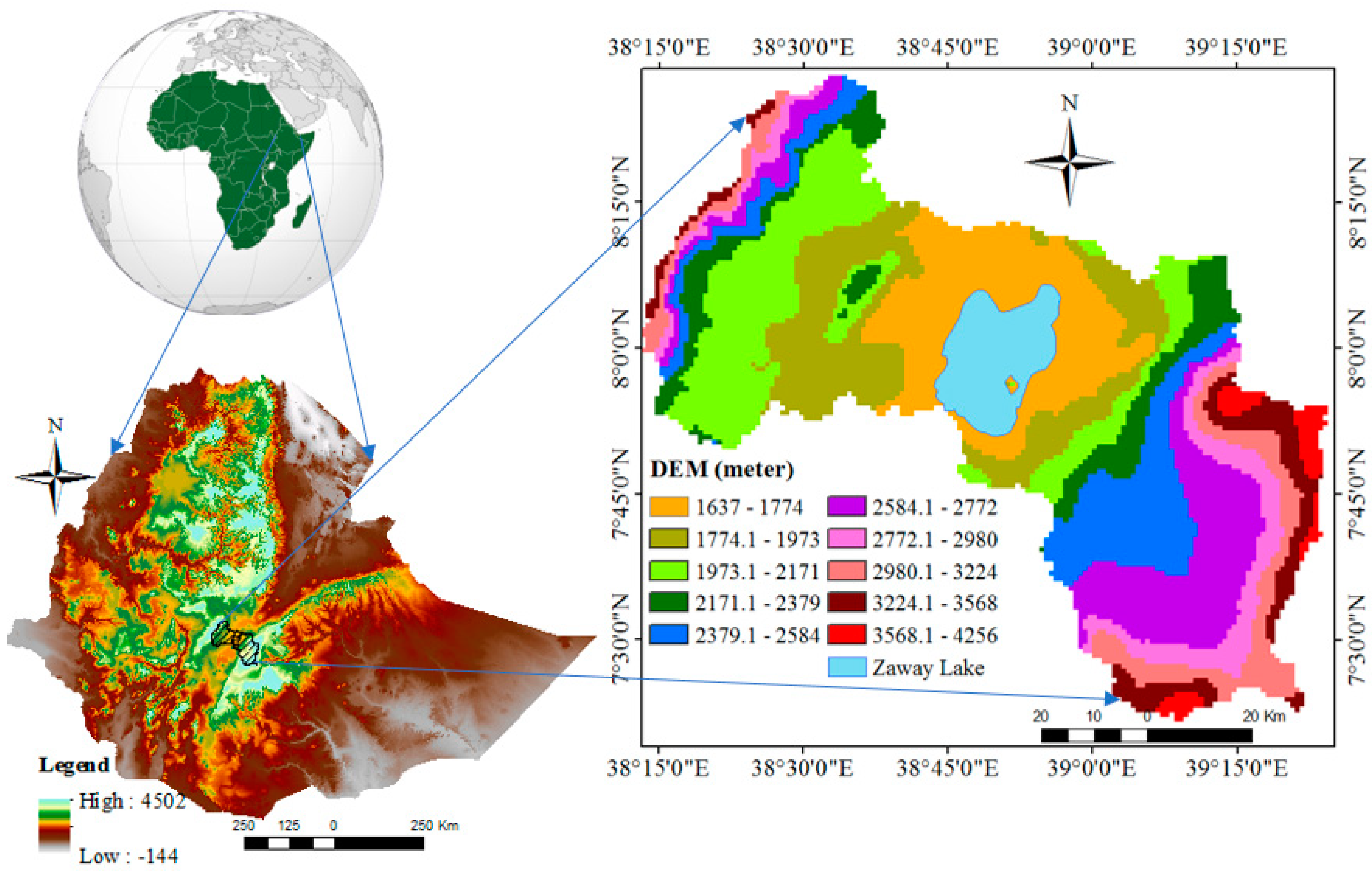
Lake Ziway is located at the northern end of the southern Rift Valley (Figure 1). The lake is the shallowest lake in the country and drains to Lake Abiyata. It is the third largest freshwater lake of the Ethiopian Rift Valley lakes and the fourth in the country. The lake has a surface area of 423 km2 and has five islands: namely Gelila, Debre Sina, Tulu Gudo, Tsedecha, and Fundro. The lake basin has a total area of 7285 km2 and geographically it extends from 7°20′54″ to 8°25′56″ latitude and 38°13′02″ to 39°24′01″ longitude. The majority of the watershed is flat to gently undulating, but is bounded by a steep slope in the eastern and southeastern escarpments and is characterized by abrupt faults. There is a topographic difference of about 2600 m between the rift floor and the highland areas (mountains) of the basin.
2.2. Climate
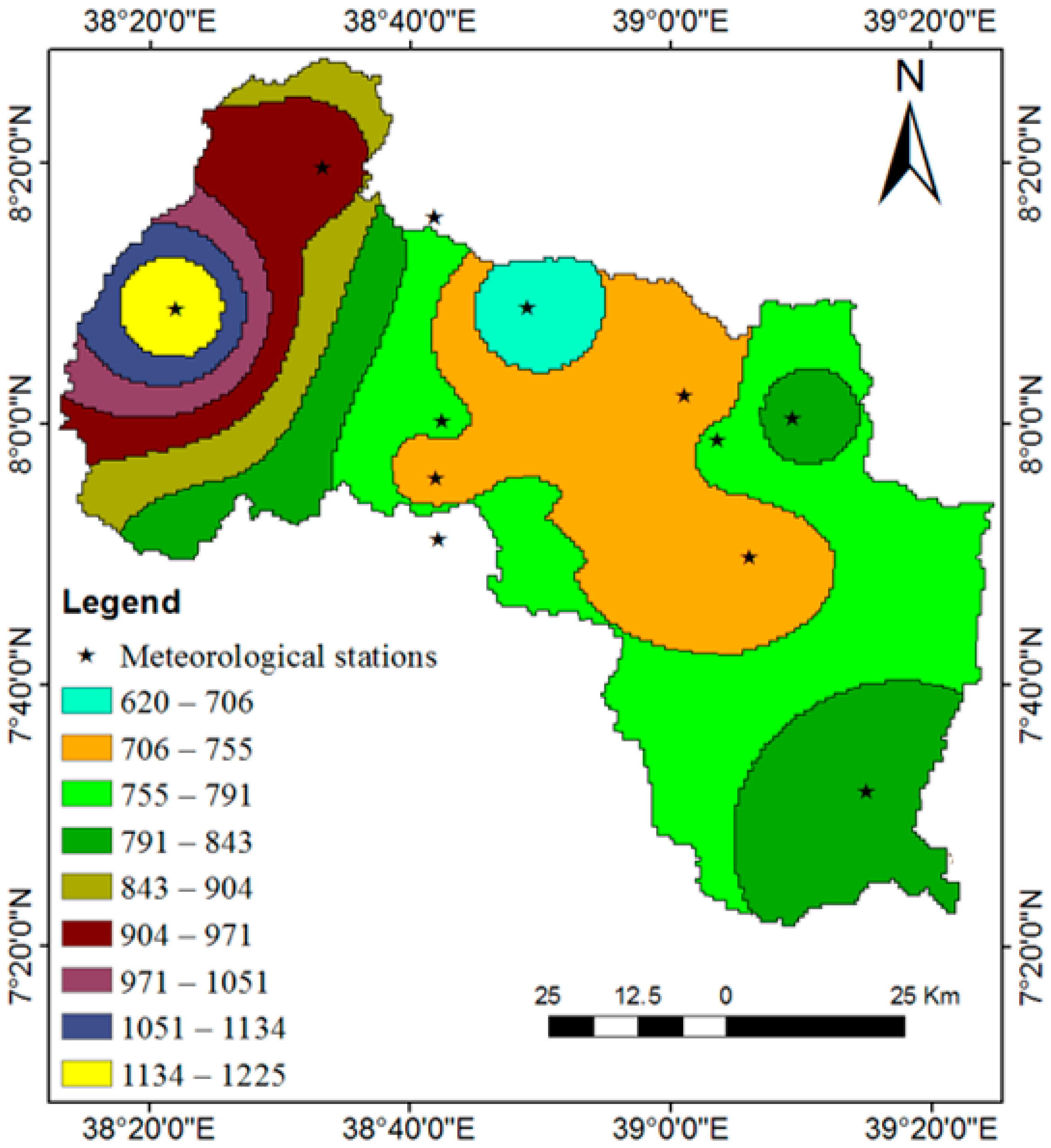
The climate of the Lake Ziway basin is dry to sub-humid or humid. The lowland area surrounding the lake is arid or semi-arid, and the highlands are sub-dry humid to humid. The basin is classified into three main seasons based on its rainfall [48]. The long rainy season is summer and is locally known as Kiremt. The Kiremt rain represents 50–70% of the mean annual total rainfall. The dry period extends between October–February, locally known as Bega. The small rainy season, known as Belg, represents 20–30% of the annual rainfall and occurs from March–May.
There are twelve meteorological stations within and near the basin namely Arata, Bekoji SF, Ketera Genet, Kulumsa, Meraro, Ogolcho, Adamitulu, Bui, Butajra, Koshe, Maki, and Ziway; and their long term (1987–2016) mean annual rainfall ranges from 620 to 1225 mm. The areal map of rainfall depth by using the inverse distance square interpolation method (IDW) is shown in Figure 2.
2.3. Hydrology
The lake is fed by two main rivers, the Katar and Maki rivers, and overflow into the Bulbula River. The Katar River is the biggest perennial river and has a total watershed area of 3350 km2. Maki River drains an area of 2433 km2 from the west and northwest of Lake Ziway. Analysis of the streamflow data indicated that as the Katar is feeding the lake with an average annual runoff volume of 401.6 Mm3, it attains a maximum discharge of 110 m3/s in the month of August and a minimum discharge of 1.6 m3/s in the month of January. Similarly, Maki River is feeding Lake Ziway with average annual runoff volume of 270.24 Mm3 and it attains its maximum discharge of 95 m3/s in the month of August. During November to January, the river bed is dry and the base flow of the river is almost nil during the severe dry seasons of the year. Regarding its outflow, Lake Ziway discharges into the Bulbula River with a mean annual runoff volume of 116.3 Mm3.
2.4. Geology, Soil, and Land Use
The geology of Lake Ziway basin is divided into four major groups of rock units that are based on age-Precambrian to Early Paleozoic crystalline basement succession rock, Mesozoic sedimentary rock, Oligocene to middle Miocene pre-rift volcanic rock and middle-Miocene to Holocene syn-and post-rift volcanic rock and unconsolidated sediments [47,49]. The soil of the Lake Ziway basin is closely related to parental material and degree of weathering [50]. The six most dominant soil types are andosols, cambisols, fluvisols leptosols, luvisols, and vertisol [47].
Regarding land use types, in the basin, agriculture has a long history. The basin as a whole is a zone of intensive agricultural activities and there is dynamic land-use changes [47]. In the year 2010, the sediment delivery rate of the western sub-basin of the lake was assessed, and from the total basin around 14% was highly eroded with an average sediment yield (SY) of 50–106 ton/ha/year, 24% had an average SY of 20–50 ton/ha/year, and the remaining 62% was slight to moderately eroded with an average SY rate of 0–20 ton/ha/year [47]. When we did a field visit and assessment for the case of Katar (eastern lake sub-basin), we observed a seriously eroded area inside the sub-catchments.
3. Methodology
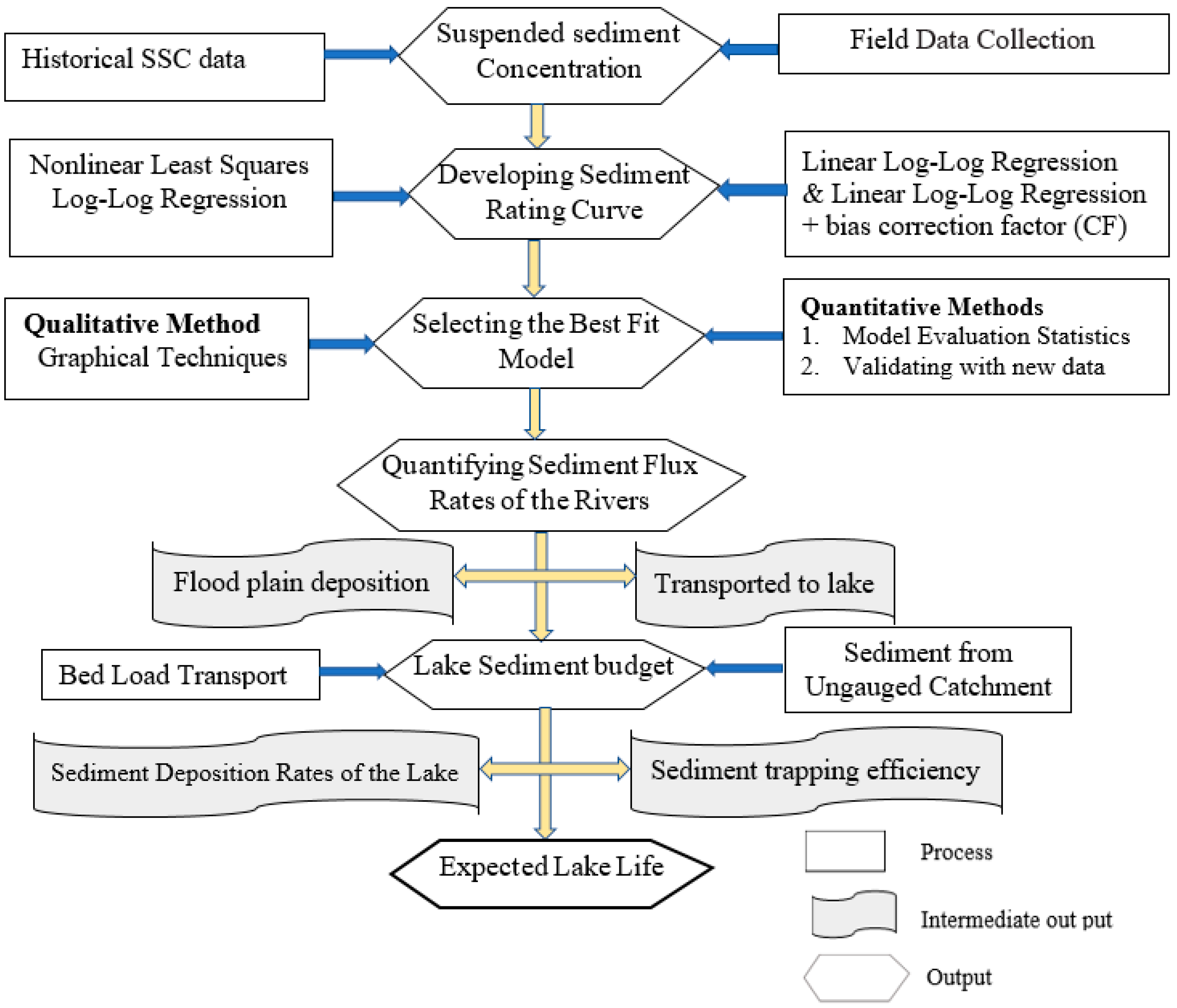
Sedimentation is of particular importance to reservoir managers, who must plan for the eventual and inevitable loss of reservoir storage. Reservoir sedimentation is the end effect of catchment erosion and the eroded soil is then transported along with any surface runoff, mainly due to precipitation, and becomes a part of the sediment load in the tributary rivers. In this study, to determine the net sediment deposition rates of Lake Ziway, both historical and newly measured sediment flow rates of its tributary rivers were used. The detailed workflow diagram of the study procedure is shown in Figure 3.
3.1. Historical Data Collection
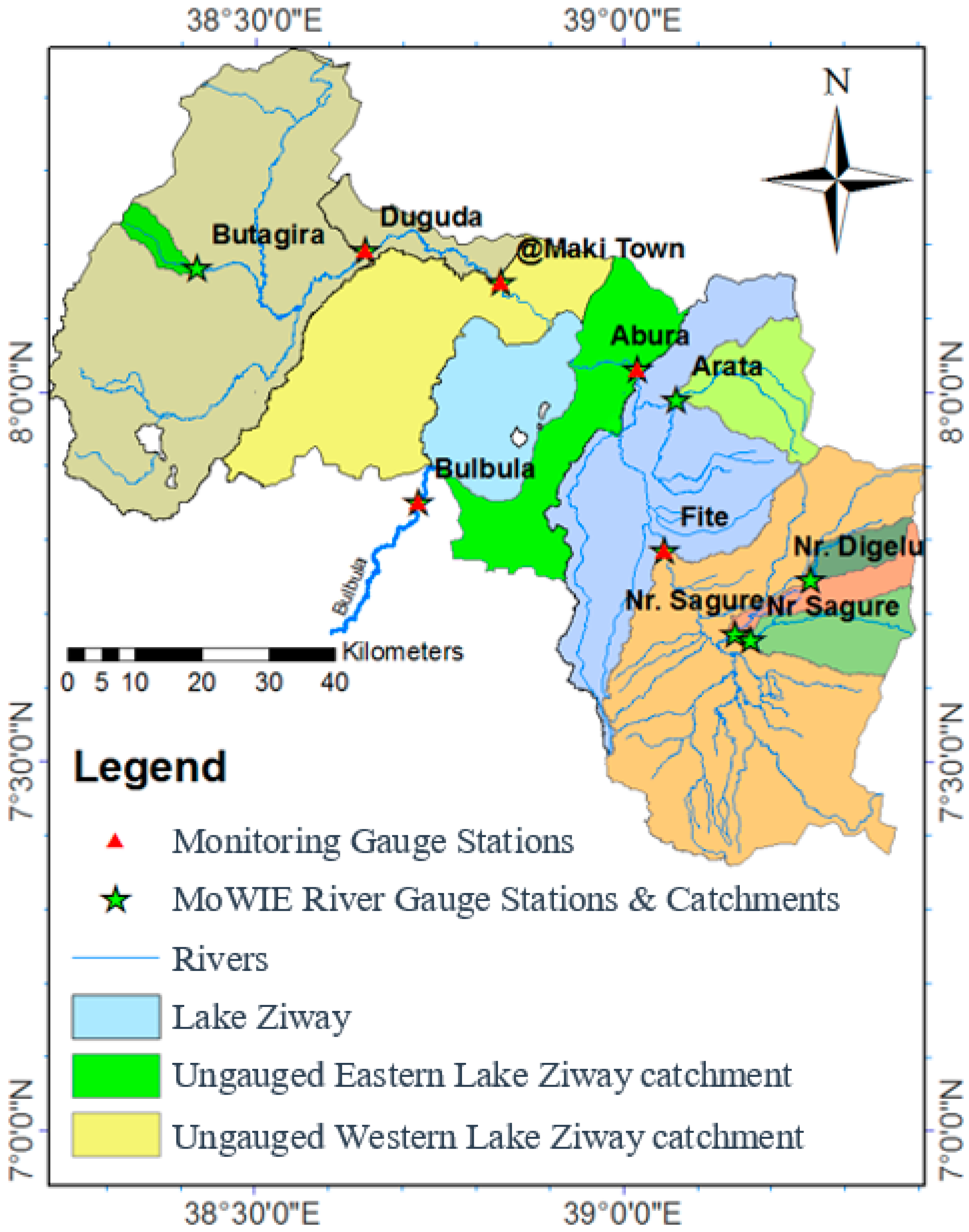
Regularly measured discharge and irregularly measured sediment concentration data were acquired from the Ethiopian Ministry of Water Irrigation and Electricity (MoWIE) for the two major rivers (Figure 4) in the Lake Ziway basin for the period of 1989 to 2013. Additional suspended sediment samples were collected from four river gauging stations and one lake outlet from mid-2016 to mid-2018 to validate the developed model.
3.2. Field Data Collection
From each monitoring station, the suspended sediment concentrations (SSCs) of the rivers were sampled in both wet and dry seasons. Suspended sediment samples (SS) were collected by dividing the river into four cross-sections of equal width and then samples were collected at different depths from each of the four sections. As the stream flow gauges are near the bridges, during high-flow season, the suspended sediment samples were collected by standing on a bridge using depth-integrated suspended-sediment samplers according to procedures outlined in Reference [51]. Each of the samples from the different depths and cross-sections was kept in a 1-pint glass bottle without overfilling the bottles. Any overfilled sample was discarded and resampled.
The sampled water taken from each station was kept in the 600 mL bottles and the gravimetric method was used to analyze the SSCs in mg/L. Vacuum filtration process was employed in the gravimetric method for filtering sediment from the samples [52]. During the high-flow season, the concentration of sediment was high, and in such cases, a pre-weighed dish was used to evaporate a measured portion of the sample to determine the weight of the residue according to procedures outlined in Reference [53].
The river cross-sectional profile was assessed in low- and medium-flow seasons using a few hydrological apparatuses, and the flow velocity of the rivers were tested by current meter. For all monitoring stations, there was a staff gauge equipped by MoWIE and used to convert the river stages into flow discharge.
3.3. Estimating the Suspended Sediment Yield through Regression Relationship
Because of the scarcity of continuous sediment data, estimates are often derived from empirical relations between river discharges and corresponding suspended sediment concentrations/loads which is called as rating curve [54] and is equated as
where Qs is suspended sediment transport (ton/day), Qw is daily stream flow (m3/s), and a and b are regression coefficient and exponent, respectively.
Log (Qs) = a + b * Log (Qw)
Sediment load calculated using the above relation has been reported as it is underestimating the actual suspended sediment loads [45]. A bias correction factor (CF) was introduced and the SSC rating curve was corrected as:
Log (Qs) = a + b * Log (Qw) + CF
Reference [45] proposed a statistical bias correction factor (CF) equal to exp(2.65S2) to reduce the degree of underestimation by rating curve with
where S2 is the variance, Ci and Ĉi are observed and predicted values, and n is the number of observations.
In this study, the normal linear log–log regression, the normal log–log regression with correction bias factor, and the non-linear least squares regression methods were used to derive the sediment yield from measured suspended solids data. Non-linear with optimization procedure is derived as:
where a, b, and c are coefficients determined through a regression and optimization procedure using the Microsoft Excel Solver Tool by setting an objective function to minimum as indicated in Reference [2].
Log (Qs) = a + b * (Log Qw)c
By using those three methods (Equations (1), (2), and (4)), sediment rating curves were developed for all monitoring stations and the most appropriate sediment rating curve was selected based on goodness-of-fit. The goodness-of-fit of the rating curves were evaluated and tested statistically by using five widely used statistics namely: coefficient of determination (R2), Nash–Sutcliffe efficiency (NSE), root mean square error (RMSE), observations standard deviation ratio (RSR), and percent bias (PBIAS). Their recommended value to test the performance of the models is shown in Table 1 [55].
Furthermore, to validate the methods, the relative errors of estimation were calculated from measured suspended sediment concentrations and the predicted suspended loads as:
The predicted and measured sediment loads were computed by plotting the graph between observed and computed data.
3.4. Estimating the Sediment Deposition on Rivers Floodplains
Floodplain upstream of the lakes can serve as sediment trapping areas as large alluvial soils can be deposited by rivers [38]. The two tributaries of Lake Ziway drain a large part of the floodplian (Figure 5) which retains most of the sediment transported and can be used as a site for intensive sand mining activities across sections of the rivers [56].
In the lake basin, the sediment trapped in the floodplain is a yield for the basin but it is not the budget for the lake [38,57], which needs to be quantified. To do this, the suspended sediment concentrations were collected on the lower and upper gauging stations of the two tributary rivers (Maki and Katar). For the case of Maki, the gauging stations Duguda and Maki were selected and for Katar, Fite, and Abura, gauging stations were also selected. The length between the two gauging stations Duguda and Maki was 41.6 km and between Fite and Abura it was around 37.5 km. To estimate the sediment deposited on the river channels per length, the sediment yield estimated in the upper gauging station is deducted from the lower gauging station and divided by the river channel length as follows:
Lastly, to estimate the net amount of sediment transported into the lake, the average per length loss rate calculated in Equation (6) is multiplied by the distance between the lower station and the lake.
3.5. Application of the Regression Relationships to Ungauged Watersheds
Around 22% of the basin with notable flat areas did not have observed suspended sediment data (Figure 4). Hence, the contribution of the ungauged basin was estimated by developing an empirical model that relates the terrain attributes namely drainage area, slope, and average annual rainfall with sediment yield [38]. From this, the three explanatory factors, the area and slope of the ungauged basins were extracted from the 30 × 30 DEM of the basin and the mean annual rainfall was determined from the basin area rainfall depth map (Figure 2).
3.6. Sediment Trap Efficiency of Lake Ziway
The limited measured suspended sediment concentrations at the Bulbula River gauging station were obtained from MoWIE and during field data collection, and SSCs of the outflow river were sampled in both wet and dry seasons. To estimate the annual suspended sediment mass leaving the lake, a rating curve was developed from data collected from the field and historically existing data.
3.7. Bedload Estimation
The total sediment load of streams usually is considered to be the sum of two components, called suspended load and bedload. In Ethiopia, most studies [38,58,59,60] ignored the bedload contribution. However, in most rivers, bedload to suspended load ratio is in the range of 10% to 30% [38,61], and in mountain rivers (high slope) ranges up to 35% of the suspended load [38,62]. In this study, the Maki and Katar rivers flow on gentle slopes for more than 13 km before joining Lake Ziway. Hence, we assumed the bedload was 10% of suspended sediment load.
3.8. Sediment Balances of Lake Ziway
Sediment balance for a lake Ziway is based on the law of conservation of mass [38,63].
where ΔV is the volume of sediment deposited inside the lake, SSin the amount of sediment transported into the lake and SSout is the amount of sediment exporting from the lake.
ΔV = SSin − SSout
For the case of Lake Ziway, the net amount of sediment deposited in the lake can be calculated as:
where SSN is the net annual sediment deposition in lake, SSg and SSu stands for annual gauged and ungauged basins sediment flow respectively, SSb stands for bedload sediment flow and SSbl is sediment outflow from the lake through the Bulbula River
SSN= SSg + SSu + SSb − SSbl
3.9. Sediment Volume and Lake SedimentTrapping Efficiency
To obtain the rate of sedimentation in the lake, an average specific weight of lake sediment is required. Sediment core samples were collected from ten points from the shore of the lake and undisturbed samples were dried for 24 h at 105 °C and the mean bulk density (BD) of 1.22 ton/m3 was determined.
The sediment trapping efficiency (Tef) of the lake was calculated as
where SYin and SYout are inflowing and outflowing sediment load (in ton/year).
4. Result and Discussion
4.1. Suspended Sediment Discharge from Gauged Catchments
Both historical and newly measured suspended sediment data were used to estimate the suspended sediment loads of the rivers. The average suspended sediment concentration of all samples was 1.9 (±1.8) g/L and the average estimated sediment yield was 3.5 (±4.8) × 103 ton/day. During strong floods in the rainy season, its suspended sediment concentration could reach up to 8600 mg/L and SY could reach up to 31.9 × 10³ ton/day. For all monitoring stations, the suspended sediment concentration was decreasing after the end of main rainy season (September) and increases at the beginning of the small rainy season (Belg). During most dry seasons, the tributary rivers carry less sediment and a clear trend in mean sediment yield was observed. This seasonal suspended sediment flow pattern observed in the basin is similar to those found by a study done in Northern Ethiopia by Reference [38] on tributaries of Lake Tana and by Reference [64] in the Geba catchment of Northern Ethiopia.
4.1.1. Sediment Rating Curve Development
To estimate the siltation rate of Lake Ziway and the sediment contribution rates of its sub-catchments, rating curves with normal linear log–log regression (Equation (1)), normal linear log–log regression with correction factor (Equation (2)), and non-linear least squares regression (Equation (4)) methods were established for all monitoring gauging stations (Figure 6).
The comparison plots between measured and computed data with three different rating curves, namely rating curve developed by normal linear log–log regression (Equation (1)), normal linear log–log regression with correction factor (Equation (2)), and non-linear least squares regression (Equation (4)) is shown in figure (Figure 7).
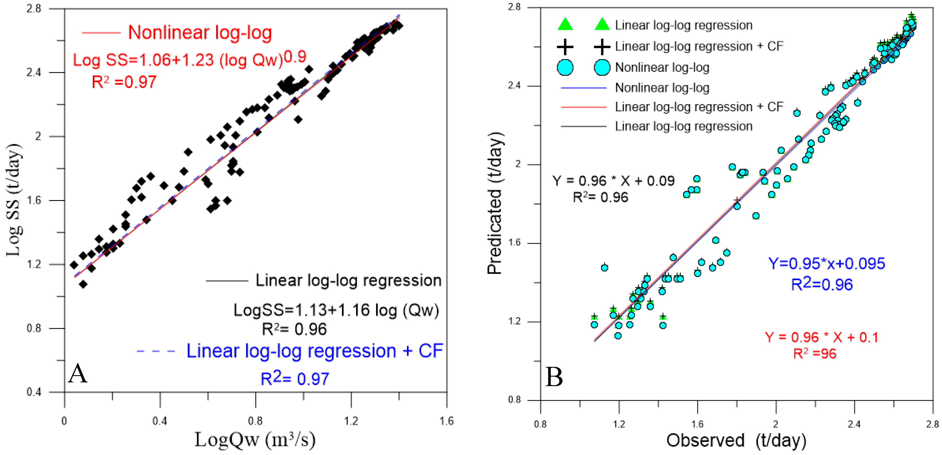
Similarly, for the lake outlet station (Bulbula River), the sediment rating curve was developed as shown in Figure 8A by using Equations (1), (2), and (4), and the comparison plot between measured and computed data is shown in Figure 8B.
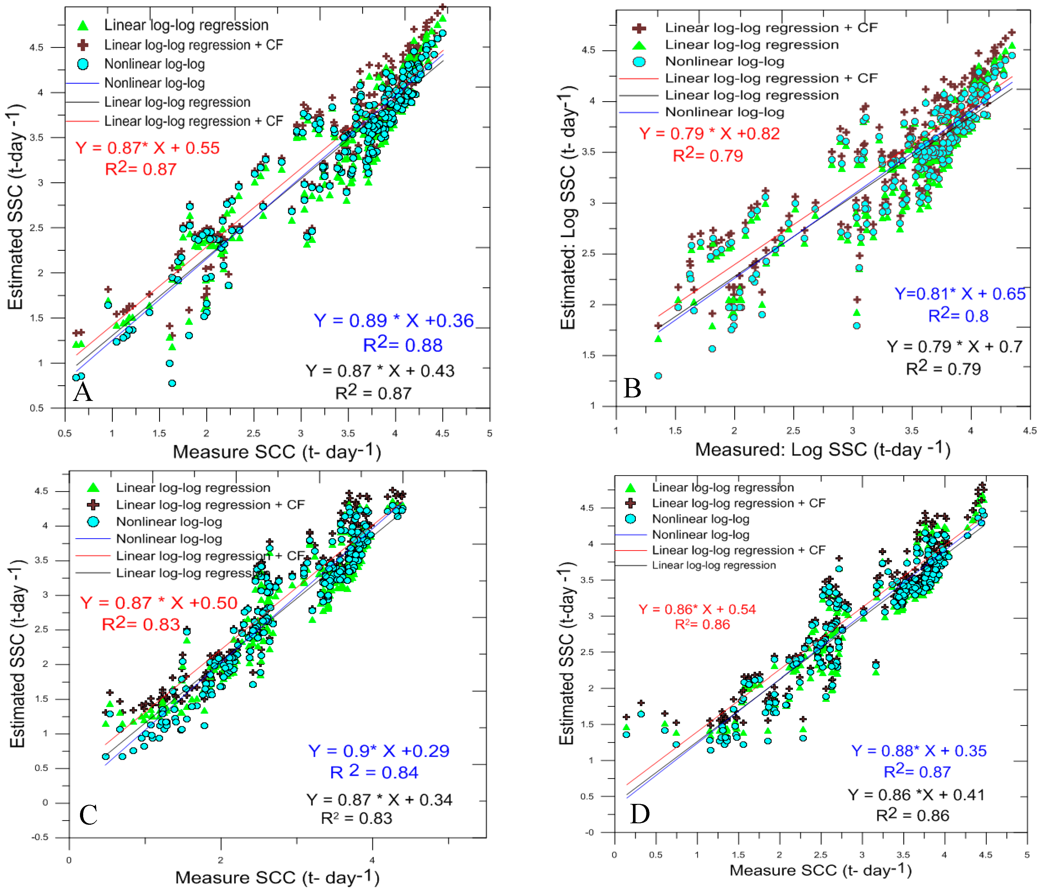
As shown in Figure 6, for all monitoring river stations, the model developed by the non-linear least squares regression method was below from both low- and high-stream flows. For medium stream flow, it was between the model developed by linear log–log regression and its corrected one. Hence, this may represent the real condition of the study basin. In the basin, the sediment concentration of the rivers did not increase proportionally with discharge (rainy phase). This can be explained by various reasons. At the beginning of the rainy season, in most parts of the basin, newly plowed land for agriculture facilitates the removal and transportation of soil by runoff. At the end of the rainy season (during river Peak low), the concentration of sediment is low due to plant cover protection of lands. Lastly, during most dry seasons, the tributary rivers carry less sediment until the rainy phase starts. In addition to this, the calculated correlation coefficient (r2) between observed and computed sediment for the model developed by linear log–log regression was also low. Hence, the time series plots graph developed in Figure 6 indicates the use of non-linear least squares regression method as a better alternative to the sediment rating curve in the prediction of sediment load.
In the literature, there are two controversial ideas concerning sediment rating curves and sediment prediction. Some state that rating curves developed based on linear log-transformed data underestimate and others present it as overestimating when compared with the corresponding observed sediment loads. To compensate its degree of underestimation, the bias correction factor was also developed. Others have stated that there is no best method to develop sediment rating curves. To validate these controversies, let us take any of the developed rating curves from Figure 6. As shown in Figure 6, the model developed by the linear method underestimates observed sediment loads for medium-flow seasons. Hence, those who propose to use the bias correction factor are applicable for this section only. In our basin, this position is the time where the rainy phase starts, and more sediment concentrations were observed. Next to that there is a point in which both curves are crossed with each other. This is the point in which both methods are predicting equal sediment loads. Therefore, the authors decided to use any type of ratings curve in these sections only. Lastly, for minimum-flow and peak-flows seasons, there are over predictions. Due to this, we suggested that unless sediment rating curves are developed for each season of the year using linear log–log regression methods, there will be a limitation in compensating for all of the seasons of the year.
The performance of the developed sediment rating curves was evaluated using model evaluation statistics and the results of goodness-of-fit test statistics were determined as follows (Table 2).
The outperformed model was selected based on minimum RMSE, RSR, and PBIAS, and maximum NSE and R2. Reference [55] recommended that if the R2 and/or NSE has a value of >0.9, 0.9 to 0.75, 0.65 to 0.75, or >0.50, the model can be rated as excellent, very good, adequate, and satisfactory, respectively, in predicting sediment yield. In this study, therefore, we found the R2 values estimated by non-linear regression method for all stations was under excellent and for linear regression under very good except the Bulbula Station (lake outlet). Based on NSE, RMSE, RSR, and PBIAS, all of the three-model predictive performances were very good. As the data used for the model development were few in number, some statistical results indicate that the three developed models have an ability to estimate equally. But compared with their magnitudes, for all statistical parameters developed, the non-linear method is better than the others, and this has been confirmed in the graphical results shown in Figure 6.
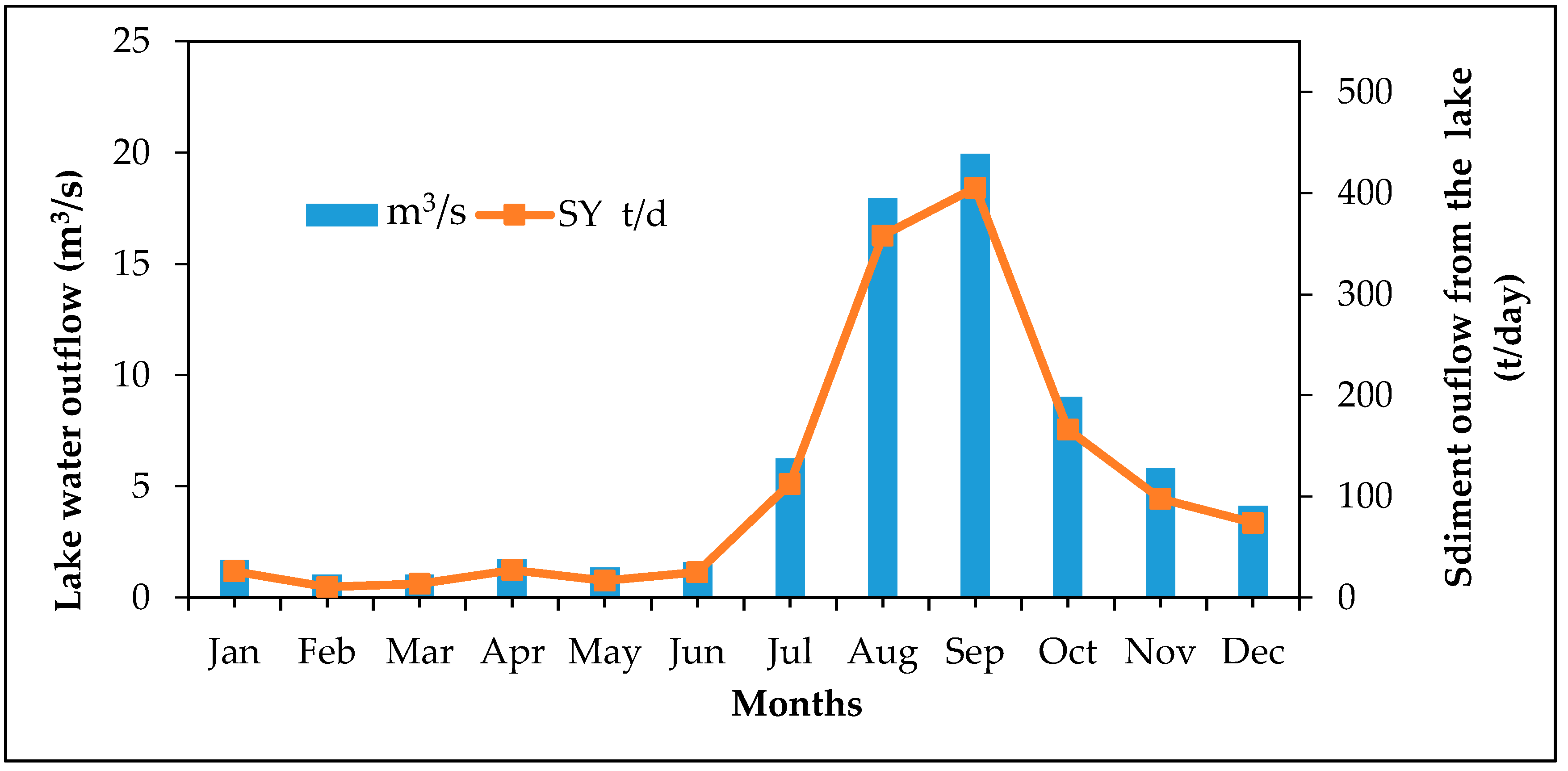
The Bulbula River is an outflow location of the lake and the determined graphical as well as statistical model results are different from the others (Figure 8 and Table 2). As shown in Figure 8, the developed sediment rating curves of the three methods and the observed and estimated sediment by the developed rating curves overlapped with each other. This indicates the model developed by all of the methods were equal in predicting the sediment load. Practically, the results may be logical. As the station is the outflow location of the lake, the sediment concentration will depend on the amount of outflow and not on the seasonal rainfall amount. As the lake has its own sediment retention period, the monthly/daily variation of sediment is due to the lake outflow rate difference but not on seasonal sediment inlet rates (Figure 9). For the case of inlet rivers, similar amounts of discharge will have different amounts of sediment concentration, and hence, a non-linear method may be an appropriate one. But for the case of the lake outlet, a model developed by any method can be used. For example some authors including Reference [8] advise to use any method to develop sediment rating curves.
By applying the developed models, the correlation of predicted and observed sediment were tested by slope and y-intercept values (Figure 7). In the model evaluation, the existence of low slope indicates the better performance. Hence, for all stream monitoring stations, the predicted performance of rating curves developed by the non-linear least squares regression method were better and the results were similar with other statistics obtained and given in Table 2.
Lastly, to validate the models, suspended sediment samples were collected from five monitoring gauging stations during the Belg rainy season of the year 2018. By using this newly measured data, the prediction error (%) of linear log–log, linear log–log with bias correction, and non-linear log–log regression methods were calculated. At the Maki monitoring station, the prediction error was +15, +23.44, and −2.8; at Duguda Station −9.97, +18.68, and −1.96; Abura −19.89, +13.16, and +3.49; Fite −14.11, +15.87, and −2.45; and for Bulbula −3.59, −1.34, and −0.25. The non-linear least squares regression method gave an error below ±3.5%. For Bulbula Station, the error was similar for all of the methods. Therefore, for all monitoring stations, the non-linear log–log regression approach was used to estimate the sediment load of the rivers. This approach was also selected during the study carried out on the Mackinaw River at Congerville, Kankakee River near Wilmington, Sangamon River near Oakford, and Illinois River in the USA by Reference [43] to estimate their sediment budgets and by Reference [65] to assess the sediment balances in the Blue Nile River Basin.
4.1.2. Predicted Sediment Concentrations in Each Monitoring Station
The estimated sediment yield by selected rating curve (non-linear regression method) for each monitoring station is given in Table 3. In this calculation, the daily mean stream flows were used to get daily sediment yields of each day.
4.2. Suspended Sediment Discharge from the Ungauged Streams
The contribution of the ungauged basin was estimated by developing a model that relates the gauged stations terrain attributes namely drainage area, slope, and average annual rainfall with annual suspended sediment yield (Figure 10).
For ungauged catchments, the model estimates the mean annual suspended sediment yield of 0.16 million ton/year. Thus, this implies an area-specific sediment yield (SSY) for ungauged catchments (1460.64 km2) as 111.55 ton/km2/year. The reason for this low sediment yield for the ungauged part of the basin may be due to it gentle slope (on average 7%). But by using such approaches, study on Lake Tana basin by Reference [38] indicates as the best relationship was established to estimate the SY of the ungauged rivers by using an average annual rainfall and catchments area.
In most studies, to predict the sediment yield of ungauged catchments, the commonly used attribute is the catchment area only [66]. From other terrain attributes, area can easily be determined if maps of appropriate scale are available Some studies in Ethiopia, for example Reference [67] in Northern Tigray, used catchment area only to estimate the sediment yield of ungauged parts. Similarly, Reference [68] developed an equation that relates SSY with catchment area for the Central and Northern Ethiopian highlands (Equation (10)).
where SSy is area-specific suspended sediment yield in t km−2 year−1; A is area in km2.
SSy = 2595A−0.29 (n = 20; r2 = 0.59)
In the absence of measured suspended and bedload sediment data, Equation (10) can be applied for Ethiopian watersheds [68] and Reference [59] applied the suggested equation to model the sedimentation rate of Lake Tana.
Hence, in our study basin, the relation of sediment yield with contributing catchment area is inversely related, and similar observations have been reported by References [38,67,68]. But when we check the applicability of the suggested equation by Reference [68] for our study area, it overestimated the sediment yield predicted for ungauged catchments by a combination of slope, rainfall, and catchment area by 180%, i.e., for an ungauged area of 1460.64 km2, the equation will give SSY of 313.63 ton/km2/year, and hence, predicting SSY with an area-only based method is not preferred for estimating the sediment yield.
The bedload contribution of ungauged parts of the basin was not considered. Since the bedload comprises the sediment that moved downstream by saltation and rolling, it requires substantial flowing velocity. But, the ungauged parts of study basin are located in the lower position of the basin with flat to gentle slopes. Hence, it cannot generate a flow that can transport the sediment in the form of bedload.
4.3. Suspended Sediment Deposited in Floodplains
A net annual suspended sediment deposited in the floodplains was estimated as 178.76 × 10³ ton/year. This corresponds to 20.6% of the total sediment yield of the basin (Table 4). The result indicates that as the average sediment aggradation rate along the Maki River and Katar were about 19.2% and 22%, respectively.
Study by [38] and [68] indicated the absence of any studies related to sediment deposition rates in floodplains in Ethiopia. Some studies in Northern Ethiopia, such as References [59,68], assumed 30% of the suspended sediment load to be deposed in floodplains. In the Kalaya River basin (Zambia), Reference [57] indicated the existence of 30% suspended sediment loss in floodplains. Similarly, Reference [69] estimated an overbank deposition of sediment on floodplains during flood events may range up to 40–50% of load delivered into the main channel system. Therefore, the suspended sediment deposited on the floodplain of our study basin is lower than what is estimated for the Kalaya River basin in Zambia and Lake Tana basin in Ethiopia by [38].
4.4. Estimated Bedload
For both tributary rivers, the bedload was calculated by assuming 10% of suspended sediment load and estimated as 174.36 × 10³ ton/year. Before joining Lake Ziway, the two tributary rivers (Maki and Katar) flow down a gentle slope for more than thirteen kilometers. Hence the contribution of bedload by those rivers may be low and the predicted value may be reasonable.
4.5. Suspended Sediment Exported Out of Lake
The suspended sediment rating curve equation was developed for the measured suspended sediment concentration at the Bulbula River gauging station (Figure 8). Application of the rating curve equation resulted in an annual suspended sediment outflow of 14,331.8 tons. The outlets start to export more sediment when excess water leaves the lake in the middle of the rainy season.
4.6. Sediment Budget and Deposition Rates of the Lake
The net annual sediment flow of the lake was calculated as the sum of the total of sediment load obtained for gauged and ungauged catchments (Figure 11). The estimated mean annual suspended deposition was 2039.59 × 103 tons. The volumetric deposition rate, which is the ratio of total sediment load to sediment bulk density of the area was computed. For the study area, the dry bulk density of 1.22 ton/m3 was determined and as the result the volumetric sediment deposition rate is 1.67 × 10⁶ m3 per year, which is equivalent to a uniform suspended sediment deposition rate of 3.98 mm/year for the mean lake surface area of 423 km2 at 1637 msl. When a constant annual rate is assumed, the lake will lose 1 m in 251.2 years. Which is higher than annual sediment deposition and lake depth loss rates estimated for Lake Tana by Reference [38] (1 m in 1000 years): [59] (1 m in 714.3 years), lower than the sediment deposition rate estimated for Lake Hawasa in Ethiopia (1 m in 83 years) by Reference [70], and almost similar with Lake Naivasha Kenya (1 m in 210 years) by Reference [71].
The amount of sediment retained by Lake Ziway (sediment trap efficiency) was estimated using Equation (9) and it was found to be about 98%. Which is high compared with study done in Northern Ethiopia for Lake Tana. For Lake Tana, the sediment trap efficiency of 63% by Reference [38] and 88% by Reference [72] was predicted. The reasons for this high sediment trapping efficiency for Lake Ziway may be due to having a small discharge and position of outflow location. More sediment is entering into the lake from the north parts of the lake and the outflow location is on its southern corner. Moreover, for Lake Tana, there are two outlets namely the Blue Nile River and the Tana Beles tunnel for hydropower production. Hence, the calculated trapping efficiency of Lake Ziway is much greater than Lake Tana.
In terms of lake volumetric loss, the total accumulated sediment is estimated as 1.67 × 10⁶ m3/year and which is about 0.106% of the total lake volume (1580 Mm3). As per this rate, the lake will lose 1% in 9.47 year to loss in 1% and in 947 years, it will lose its total volume. Which is lower than the estimated global average rate for annual loss of reservoir capacity of 1% [73]. Similarly, the estimated per year volume loss of Lake Ziway is lower compared with Lake Tana by Reference [38] and for the Ethiopian Rift Valley Lake Hawassa by Reference [70].
4.7. Uncertainties in Sediment Budget Calculation
Due to lack of instantaneous flow measurement, the sediment rating curve was developed based on daily average stream and sediment flow rates. Moreover, the estimated bedload accounts for 10% of the sediment entering into the lake through the main rivers, and which had not been directly measured in the studies. The floodplain deposition of the sediment is considered as uniform upon its length. The future lake sedimentation rates and its half-life is predicted by assuming the basin’s rainfall pattern with constant trends. So, there may be uncertainties with this assumption.
5. Conclusions
In this study, sediment transport rates were estimated for five monitoring gauge stations by developing rating curves with normal linear log–log regression, normal log–log regression with correction bias factor, and non-linear log–log regression. The best-fit model was tested and evaluated qualitatively by time-series plots, quantitatively by using watershed model evaluation statistics, and validated by calculating the prediction errors. On tributary river monitoring stations, the non-linear log–log regression method estimated the sediment yield better than others, and for the lake out flow monitoring station, all methods predicted equally.
The model estimated the gross sediment load transported into the lake as 2080.93 × 103 ton/year. The sediment load exported out of the lake by the Bulbula River was 41,339.4 ton/year, and as a result, a net annual sediment mass of 2039.6 × 103 ton/year was deposited in the lake.
In terms of lake storage capacity loss, the annual reduction due to siltation is found to be 0.106% and 3.98 mm in terms of lake depth. The lake has a sediment trapping efficiency of 98% and the expected half lifetime of the lake is 473.5 years.
Author Contributions
A.O.A. conceived the study. He has also participated in the design of the study, carried out the data collection, analysis of data, and performed the statistical analysis. A.M.M. and B.C. participated in the sequence alignment of the draft manuscript. They also participated in its design and coordination, and helped to draft and edit the manuscript. All authors read and approved the final manuscript.
Funding
The study was financed by Addis Ababa University Institute of Technology.
Acknowledgments
We would like to thank the Ethiopian National Meteorological Service Agency and Ministry of Water, Irrigation, and Electricity for providing the necessary data.
Conflicts of Interest
The authors declare no conflict of interest.
References
- Abdallah, M.; Stamm, J. Evaluation of Sudanese Eastern Nile Reservoirs Sedimentation. Dresdner Wasserbaukolloquium 2012, 35, 285–297. [Google Scholar]
- Asselman, N.E.M. Fitting and Interpretation of Sediment Rating Curves. J. Hydrol. 2000, 234, 228–248. [Google Scholar] [CrossRef]
- Wisser, D.; Frolking, S.; Hagen, S.; Bierkens, M.F.P. Beyond peak reservoir storage? A global estimate of declining water storage capacity in large reservoirs. Water Resour. Res. 2013, 49, 5732–5739. [Google Scholar] [CrossRef] [Green Version]
- Kim, S.M.; Jang, T.I.; Kang, M.S.; Im, S.J.; Park, S.W. GIS-based lake sediment budget estimation taking into consideration land use change in an urbanizing catchment area. Environ. Earth Sci. 2014, 71, 2155–2165. [Google Scholar] [CrossRef]
- Walling, D.E.; Collins, A.L. The catchment sediment budget as a management tool. Environ. Sci. Policy 2008, 11, 136–143. [Google Scholar] [CrossRef]
- Hajigholizadeh, M.; Melesse, A.M.; Fuentes, H. Erosion and Sediment Transport Modelling in Shallow Waters: A Review on Approaches, Models and Applications. Int. J. Environ. Res. Public Health 2018, 15, 518. [Google Scholar] [CrossRef] [PubMed]
- Osore, A.; Moges, A. Extent of Gully Erosion and Farmer’s Perception of Soil Erosion in Alalicha Watershed, Southern Ethiopia. J. Environ. Earth Sci. 2014, 4, 74–81. [Google Scholar]
- Sadeghi, S.H.; Saeidi, P. Reliability of sediment rating curves for a deciduous forest watershed in Iran. Hydrol. Sci. J. 2010, 55, 821–831. [Google Scholar] [CrossRef] [Green Version]
- Mhiret, D.; Ayana, E.; S Legesse, E.; Moges, M.; Tilahun, S.; Moges, M. Estimating reservoir sedimentation using bathymetric differencing and hydrologic modeling in data scarce Koga watershed, Upper Blue Nile, Ethiopia. J. Agric. Environ. Int. Dev. 2016, 110, 413–427. [Google Scholar] [CrossRef]
- Defersha, M.B.; Melesse, A.M. Effect of rainfall intensity, slope and antecedent moisture content on sediment concentration and sediment enrichment ratio. CATENA 2012, 90, 47–52. [Google Scholar] [CrossRef]
- Mekonnen, M.; Melesse, A.M. Soil Erosion Mapping and Hotspot Area Identification Using GIS and Remote Sensing in Northwest Ethiopian Highlands, Near Lake Tana. In Nile River Basin; Springer: Dordrecht, The Netherlands, 2011; pp. 207–224. ISBN 978-94-007-0688-0. [Google Scholar]
- Maalim, F.K.; Melesse, A.M. Modelling the impacts of subsurface drainage on surface runoff and sediment yield in the Le Sueur Watershed, Minnesota, USA. Hydrol. Sci. J. 2013, 58, 570–586. [Google Scholar] [CrossRef] [Green Version]
- Melesse, A.M.; Ahmad, S.; McClain, M.E.; Wang, X.; Lim, Y.H. Suspended sediment load prediction of river systems: An artificial neural network approach. Agric. Water Manag. 2011, 98, 855–866. [Google Scholar] [CrossRef]
- Setegn, S.; Dargahi, B.; Srinivasan, R.; Melesse, A.M. Modeling of Sediment Yield from Anjeni-Gauged Watershed, Ethiopia Using SWAT Model1. J. Am. Water Resour. Assoc. 2010, 46, 514–526. [Google Scholar] [CrossRef]
- Abtew, W.; Melesse, A.M. Landscape Changes Impact on Regional Hydrology and Climate. In Landscape Dynamics, Soils and Hydrological Processes in Varied Climates; Springer Geography; Springer: Cham, Switzerland, 2016; pp. 31–50. ISBN 978-3-319-18786-0. [Google Scholar]
- Anwar, A.A.; Seifu, A.T.; Essayas, K.A.; Abeyou, W.W.; Tewodros, T.A.; Shimelis, B.D.; Melesse, A.M. Climate Change Impact on Sediment Yield in the Upper Gilgel Abay Catchment, BlueNile Basin, Ethiopia. In Landscape Dynamics, Soils and Hydrological Processes in Varied Climates; Springer International Publishing: Cham, Switzerland, 2015; Volume 7, pp. 615–644. [Google Scholar]
- Defersha, M.B.; Quraishi, S.; Melesse, A.M. Interrill erosion, runoff and sediment size distribution as affected by slope steepness and antecedent moisture content. Hydrol. Earth Syst. Sci. Discuss. 2010, 7, 6447–6489. [Google Scholar] [CrossRef]
- Dessu, S.; Melesse, A.M. Modelling the rainfall–runoff process ofthe Mara River basin using the soil and water assessment tool. Hydrol. Process. 2012, 26, 4038–4049. [Google Scholar] [CrossRef]
- Dessu, S.; Melesse, A.M.; Bhat, M.; McClain, M.E. Assessment of water resources availability and demand in the Mara River basin. CATENA 2014, 115, 104–114. [Google Scholar] [CrossRef]
- Grey, O.; St, F.; Webber, D.; Setegn, S.; Melesse, A.M. Application of the soil and water assessment tool (SWAT model) on a small tropical island (Great River watershed, Jamaica) as a tool in integrated watershed and coastal zone management. Int. J. Trop. Biol. Conserv. 2014, 62, 293–305. [Google Scholar]
- Melesse, A.M.; Graham, W.D.; Jordan, J.D. Spatially Distributed Watershed Mapping and Modeling: GIS-based Storm Runoff and Hydrograph Analysis: (part 2). J. Spat. Hydrol. 2003, 3, 2–28. [Google Scholar]
- Wang, X.; Garza, J.; Whitney, M.; Melesse, A.; Yang, W. Prediction of Sediment Source Areas within Watersheds as Affected by Soil Data Resolution, In: Environmental Modelling; Nova Science Publishers, Inc.: Hauppauge, NY, USA, 2008; pp. 151–185. [Google Scholar]
- Setegn, S.G.; Srinivasan, R.; Dargahi, B.; Melesse, A.M. Spatial delineation of soil erosion vulnerability in the Lake Tana Basin, Ethiopia. Hydrol. Process. 2009, 23, 3738–3750. [Google Scholar] [CrossRef]
- Msaghaa, J.J.; Melesse, A.M.; Ndomba, P.M. Modeling Sediment Dynamics: Effect of Land Use, Topography, and Land Management in the Wami-Ruvu Basin, Tanzania. In Nile River Basin; Springer: Cham, Switzerland, 2014; pp. 165–192. ISBN 978-3-319-02719-7. [Google Scholar]
- De Vente, J.; Poesen, J.; Verstraeten, G.; Govers, G.; Vanmaercke, M.; Van Rompaey, A.; Arabkhedri, M.; Boix-Fayos, C. Predicting soil erosion and sediment yield at regional scales: Where do we stand? Earth-Sci. Rev. 2013, 127, 16–29. [Google Scholar] [CrossRef]
- Tilahun, S.A.; Guzman, C.D.; Zegeye, A.D.; Ayana, E.K.; Collick, A.S.; Yitaferu, B.; Steenhuis, T.S. Spatial and Temporal Patterns of Soil Erosion in the Semi-humid Ethiopian Highlands: A Case Study of Debre Mawi Watershed. In Nile River Basin; Springer: Cham, Swizterland, 2014; pp. 149–163. ISBN 978-3-319-02719-7. [Google Scholar]
- Yesuf, H.; Alamirew, T.; Melesse, A.M.; Assen, M. Bathymetric Mapping for Lake Hardibo in Northeast Ethiopia Using Sonar. Int. J. Water Sci. 2012, 1, 1–9. [Google Scholar] [CrossRef]
- Yesuf, H.; Alamirew, T.; Melesse, A.M.; Assen, M. Bathymetric study of Lake Hayq, Ethiopia. Lakes Reserv. Res. Manag. 2013, 18, 155–165. [Google Scholar] [CrossRef]
- Moges, M.M.; Abay, D.; Engidayehu, H. Investigating reservoir sedimentation and its implications to watershed sediment yield: The case of two small dams in data-scarce upper Blue Nile Basin, Ethiopia. Lakes Reserv. Sci. Policy Manag. Sustain. Use 2018, 23, 217–229. [Google Scholar] [CrossRef]
- Wischmeir, W.H. Predicting Rainfall-erosion Losses from Cropland East of the Rocky Mountain, Guide for Selection of Practices for Soil and Water Conservation. Agric. Handb. 1965, 282, 47. [Google Scholar]
- Steenhuis, S.; Collick, S.; Easton, M.; Leggesse, S.; Bayabil, K.; White, E.D.; Awulachew, S.B.; Adgo, E.; Ahmed, A.A. Predicting discharge and sediment for the Abay (Blue Nile) with a simple model. Hydrol. Process. 2009, 23, 3728–3737. [Google Scholar] [CrossRef]
- Syvitski, J.P.; Morehead, M.D.; Bahr, D.B.; Mulder, T. Estimating fluvial sediment transport: The rating parameters. Water Resour. Res. 2000, 36, 2747–2760. [Google Scholar] [CrossRef] [Green Version]
- Warrick, J.A. Trend analyses with river sediment rating curves. Hydrol. Process. 2015, 29, 936–949. [Google Scholar] [CrossRef]
- Bordbar, A.; Fuladipanah, M. Sediment Rating Curve Modification (Case Study: Marun Dam, Behbahan, Iran). Indian J. Fundam. Appl. Life Sci. 2014, 4, 2345–2351. [Google Scholar]
- Lee, J.-S.; Kim, C.-G.; You, E.-G. Derivation Method of Rating Curve and Relationships for Flow Discharge-Total Sediment at Small-Midium Streams in Agrarian Basin. J. Korea Contents Assoc. 2015, 15, 544–555. [Google Scholar] [CrossRef]
- Costa, A.; Anghileri, D.; Molnar, P. A Process–Based Rating Curve to model suspended sediment concentration in Alpine environments. Hydrol. Earth Syst. Sci. Discuss. 2017, 1–23. [Google Scholar] [CrossRef] [Green Version]
- Moges, M.A.; Zemale, F.A.; Alemu, M.L.; Ayele, G.K.; Dagnew, D.C.; Tilahun, S.A.; Steenhuis, T.S. Sediment concentration rating curves for a monsoonal climate: Upper Blue Nile Basin. SOIL Discuss. 2015, 2, 1419–1448. [Google Scholar] [CrossRef]
- Lemma, H.; Admasu, T.; Dessie, M.; Fentie, D.; Deckers, J.; Frankl, A.; Poesen, J.; Adgo, E.; Nyssen, J. Revisiting lake sediment budgets: How the calculation of lake lifetime is strongly data and method dependent. Earth Surf. Process. Landf. 2017, 43, 593–607. [Google Scholar] [CrossRef]
- Ayele, G.T.; Teshale, E.Z.; Yu, B.; Rutherfurd, I.D.; Jeong, J. Streamflow and Sediment Yield Prediction for Watershed Prioritization in the Upper Blue Nile River Basin, Ethiopia. Water 2017, 9, 782. [Google Scholar] [CrossRef]
- Yesuf, H.M.; Assen, M.; Alamirew, T.; Melesse, A.M. Modeling of sediment yield in Maybar gauged watershed using SWAT; northeast Ethiopia. CATENA 2015, 127, 191–205. [Google Scholar] [CrossRef]
- Setegn, S.G.; Srinivasan, R.; Melesse, A.M.; Dargahi, B. SWAT model application and prediction uncertainty analysis in the Lake Tana Basin, Ethiopia. Hydrol. Process. 2010, 24, 357–367. [Google Scholar] [CrossRef]
- Aga, A.O.; Chane, B.; Melesse, A.M. Soil Erosion Modelling and Risk Assessment in Data Scarce Rift Valley Lake Regions, Ethiopia. Water 2018, 10, 1684. [Google Scholar] [CrossRef]
- Demissie, M.; Renjie, X.; Laura, K.; Nani, B. The Sediment Budget of the Illinois River; Report for Illinois State Water Survey—2204; Griffith Drive: Champaign, IL, USA, 2004; pp. 1–59. [Google Scholar]
- Achitea, M.; Ouillon, S. Suspended sediment transport in a semiarid watershed, Wadi Abd, Algeria (1973–1995). J. Hydrol. 2007, 343, 187–202. [Google Scholar] [CrossRef]
- Ferguson, R.I. River Loads Underestimated by Rating Curves. Water Resour. Res. 1986, 22, 74–76. [Google Scholar] [CrossRef]
- Harrington, S.T.; Harrington, J.R. An assessment of the suspended sediment rating curve approach for load estimation on the Rivers Bandon and Owenabue, Ireland. Geomorphology 2013, 185, 27–38. [Google Scholar] [CrossRef]
- MOWR The Federal Democratic Republic of Ethiopia-Ministry of Water Resources. Rift Valley Lakes Basin Integrated Resources Development Master Plan Study Project. Part 1 and 2, Halcrow Group Limited and Generation Integrated Rural Development Consultants; Unpublished Document; MOWR The Federal Democratic Republic of Ethiopia-Ministry of Water Resources: Addis Ababa, Ethiopia, 2010.
- Legesse, D. Analysis of the Hydrological Response of the Ziway–Shala Lake Basin (Main Ethiopian Rift) to Changes in Climate and Human Activities. Ph.D. Thesis, Univ. d’Aix-Marseille III, Aix-en-Provenece, France, 2002. [Google Scholar]
- Ayenew, T. The Hydrogeological System of the Lake District basin. Central Main Ethiopian Rift. Ph.D. Thesis, Free University of Amsterdam, Amsterdam, The Netherlands, 1998. [Google Scholar]
- Makin, M.J.; Kingham, T.J.; Waddams, A.E.; Birchall, C.J.; Eavis, B.W. Prospects for irrigation development around Lake Zwai, Ethiopia. In Land Resource Study; Land Resources Division, Ministry of Overseas Development: Surbiton, UK, 1976. [Google Scholar]
- Edwards, T.; Glysson, G. Field Methods for Measurement of Fluvial Sediment; Open File Report 86-531; U.S. Geological Survey: Reston, VA, USA, 1988; pp. 1–132.
- ASTM (American Society of Testing and Materials). Standard Methods for Determining Sediment Concentrations in Water Samples; D 3977-97; American Society of Testing and Materials (ASTM): West Conshohocken, PA, USA, 2007; Volume 11.02. [Google Scholar]
- Ongley, E.D.; Nations, F.; A.O. of the U. Control of Water Pollution from Agriculture; Food & Agriculture Org.: Rome, Italy, 1996; ISBN 978-92-5-103875-8. [Google Scholar]
- Zhang, K.; Zhang, W.; Li, J.; Shi, Z.; Pu, S. Relation between precipitation and sediment transport in the Dasha River Watershed. Chin. Geogr. Sci. 2004, 14, 129–134. [Google Scholar] [CrossRef]
- Moriasi, D.N.; Arnold, J.G.; Liew, M.W.V.; Bingner, R.L.; Harmel, R.D.; Veith, T.L. Model Evaluation Guidelines for Systematic Quantification of Accuracy in Watershed Simulations. Trans. ASABE 2007, 50, 885–900. [Google Scholar] [CrossRef]
- EFDR RVLA. The Federal Democratic Republic of Ethiopia—Rift Valley Lakes Basin Authorty: Lake Ziway Basin Integrated Watershed Management Feasibility Study; EFDR RVLA: Hawassa, Ethiopia, 2016.
- Walling, D.; Collins, A.L.; Sichingabula, H.M.; Leeks, G.J.L. Integrated assessment of catchment suspended sediment budgets: A Zambian example. Land Degrad. Dev. 2001, 12, 387–415. [Google Scholar] [CrossRef]
- Delmas, M.; Cerdan, O.; Cheviron, B.; Mouchel, J.-M.; Eyrolle, F. Sediment export from French rivers to the sea. Earth Surf. Process. Landf. 2012, 37, 754–762. [Google Scholar] [CrossRef]
- Engida, A. Hydrological and Suspended Sediment Modeling in the Lake Tana Basin, Ethiopia. Ph.D. Thesis, University of Grenoble, Saint-Martin-d’Hères, France, 2010. [Google Scholar]
- Vanmaercke, M.; Poesen, J.; Broeckx, J.; Nyssen, J. Sediment yield in Africa. Earth-Sci. Rev. 2014, 136, 350–368. [Google Scholar] [CrossRef] [Green Version]
- Church, M. Bed Material Transport and the Morphology of Alluvial River Channels. Annu. Rev. Earth Planet. Sci. 2006, 34, 325–354. [Google Scholar] [CrossRef]
- Sitaula, B.; Garde, M.; Burbank, D.W.; Oskin, M.; Heimsath, A.; Gabet, E. Bedload-to-suspended load ratio and rapid bedrock incision from Himalayan Landslide-dam lake record. Quat. Res. 2007, 68, 111–120. [Google Scholar] [CrossRef]
- Nyssen, J.; Poesen, J.; Moeyersons, J.; Haile, M.; Deckers, J. Dynamics of soil erosion rates and controlling factors in the Northern Ethiopian Highlands—Towards a sediment budget. Earth Surf. Process. Landf. 2008, 33, 695–711. [Google Scholar] [CrossRef]
- Zenebe, A.; Vanmaercke, M.; Poesen, J.; Verstraeten, G.; Haregeweyn, N.; Haile, M.; Amare, K.; Deckers, J.; Nyssen, J. Spatial and temporal variability of river flows in the degraded semi-arid tropical mountains of northern Ethiopia. Z. Geomorphol. 2013, 57, 143–169. [Google Scholar] [CrossRef]
- Ali, Y.; Crosato, A.; Mohamed, Y.; Abdalla, S.; Wright, N. Sediment balances in the Blue Nile River Basin. Int. J. Sedim. Res. 2014, 29, 316–328. [Google Scholar] [CrossRef]
- Lahlou, A. The Silting of Morocaan Dams. In Sediment Budgets: Proceedings of the Symposium, Porto Alegre, Brazil, 11–15 December 1988; Bordas, M.P., Walling, D.E., Eds.; IAHS: Wallingford, UK, 1988; pp. 71–77. [Google Scholar]
- Tamene, L.; Park, S.J.; Dikau, R.; Vlek, P.L.G. Reservoir siltation in the semi-arid highlands of northern Ethiopia: Sediment yield–catchment area relationship and a semi-quantitative approach for predicting sediment yield. Earth Surf. Process. Landf. 2006, 31, 1364–1383. [Google Scholar] [CrossRef]
- Nyssen, J.; Poesen, J.; Moeyersons, J.; Deckers, J.; Haile, M.; Lang, A. Human impact on the environment in the Ethiopian and Eritrean highlands—A state of the art. Earth-Sci. Rev. 2004, 64, 273–320. [Google Scholar] [CrossRef]
- Walling, D.; Horowitz, A. Sediment Budgets: Proccedings of Symposium Held during the Seventh IAHS Scientific Assembly at Foz do Ignaçu, Brazil; IAHS Publ.: Wallingford, UK, 2005; Volume 291. [Google Scholar]
- Belete, M. The Impact of Sedimentation and Climate Variability on the Hydrological Status of Lake Hawassa, South Ethiopia. Ph.D. Thesis, Universität Bonn, Bonn, Germany, 2013. [Google Scholar]
- Rupasingha, R.A. Use of GIS and RS for Assessing Lake Sedimentation Processes. Case Study for Naivasha Lake, Kenya. Master’s Thesis, International Institute for Geo-Information Science and Earth Observation Enschede, Enschede, The Netherlands, 2002. [Google Scholar]
- Zimale, F.A.; Mogus, M.A.; Alemu, M.L.; Ayana, E.K.; Demissie, S.S.; Tilahun, S.A.; Steenhuis, T.S. Calculating the sediment budget of a tropical lake in the Blue Nile basin: Lake Tana. SOIL Discuss. 2016, 1–32. [Google Scholar] [CrossRef] [Green Version]
- Douglas, B.; Michael, S.; Stephen, P. Sea level rise: History and consequences. Int. Geophys. 2001, 75, 1–232. [Google Scholar]
Figure 1.
Location of the Lake Ziway basin in the Ethiopian Rift Valley.

Figure 2.
Spatially interpolated long-term average annual rainfall depth (1989–2016) of the Lake Ziway basin.
Figure 2.
Spatially interpolated long-term average annual rainfall depth (1989–2016) of the Lake Ziway basin.

Figure 3.
The workflow diagram used for the study. Suspended sediment concentration, (SSC).

Figure 4.
Ziway Lake basin river monitoring gauge stations collected from the Ethiopian Ministry of Water Irrigation and Electricity (MoWIE).
Figure 4.
Ziway Lake basin river monitoring gauge stations collected from the Ethiopian Ministry of Water Irrigation and Electricity (MoWIE).

Figure 5.
Floodplain area of the lower Maki River.
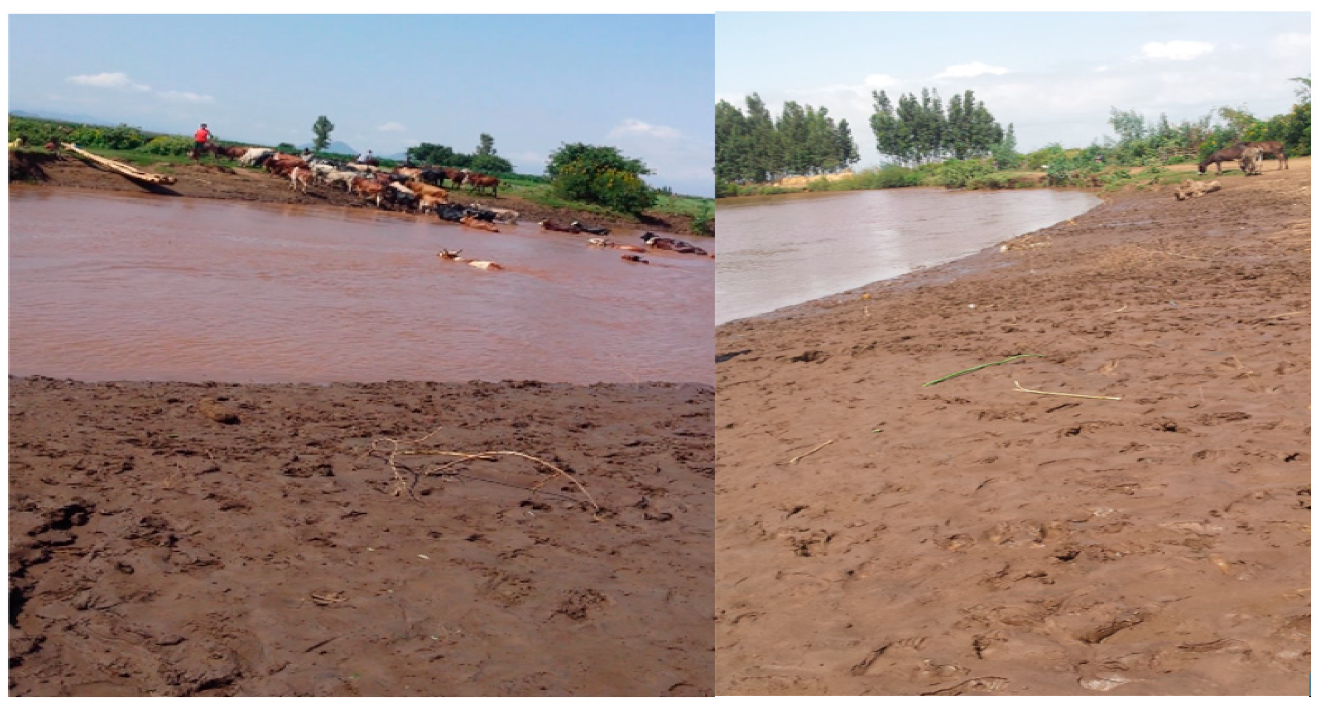
Figure 6.
The developed rating curves (A) at station Duguda; (B) Maki; (C) Abura; and (D) Fite.

Figure 7.
Predicted and observed SSCs at station (A) Duguda; (B) Maki; (C) Abura; and (D) Fite.

Figure 8.
(A) The developed rating curves for station Bulbula; and (B) Predicted and observed SSCs.

Figure 9.
Suspended sediment concentration (SSC) and lake outlets.

Figure 10.
Relationship of mean annual SSY with the product of catchment area, slope, and average annual rainfall.
Figure 10.
Relationship of mean annual SSY with the product of catchment area, slope, and average annual rainfall.

Figure 11.
Sediment budget calculated for Lake Ziway.


Table 1.
General performance ratings for recommended statistics to evaluate models [55].
Table 1.
General performance ratings for recommended statistics to evaluate models [55].
| Statistics | Performance Rating | ||||
|---|---|---|---|---|---|
| Excellent | Very Good | Good | Fair | Unsatisfactory | |
| (0.9–1) | (0.75–0.9) | (0.65–0.75) | (0.5–0.65) | (0–0.5) | |
| (0.9–1) | (0.75–0.9) | 0.65–0.75) | (0.5–0.65) | (−∞–0.5) | |
| (0–0.25) | (0.25–0.5) | (0.5–0.6) | (0.6–0.7) | (0.7–+∞) | |
| (0–0.25) | (0.25–0.5) | (0.5–0.6) | (0.6–0.7) | (0.7–+∞) | |
| (0–±5) | (±5–±15) | (±15–±30) | (±30–±55) | (±55–±∞) | |
SSC, daily measured suspended sediment load (ton/day); N, number of samples; R2, coefficient of determination; NSE, Nash–Sutcliffe efficiency; RMSE, root mean square error; RSR, observations standard deviation ratio; PBIAS, percent bias.
Table 2.
Developed rating curves for river monitoring stations.
| Rating Curve | Stations | |||||
|---|---|---|---|---|---|---|
| Maki | Duguda | Abura | Fite | Bulbula | ||
| Linear log-log Regression Log (SS) = a + b * log (Qw) | R2 | 0.79 | 0.87 | 0.88 | 0.86 | 0.96 |
| NSE | 0.79 | 0.87 | 0.85 | 0.86 | 0.96 | |
| RSR | 0.46 | 0.36 | 0.38 | 0.37 | 0.21 | |
| PBIAS | 0.23 | 0.15 | 0.74 | 0.29 | −0.03 | |
| RMSE | 0.33 | 0.32 | 0.35 | 0.34 | 0.08 | |
| Linear log-log Regression + CF Log (SS) = a + b * log (Qw) + CF | CF | 0.1 | 0.12 | 0.15 | 0.13 | 0.01 |
| R2 | 0.89 | 0.93 | 0.92 | 0.92 | 0.97 | |
| NSE | 0.77 | 0.86 | 0.83 | 0.85 | 0.96 | |
| RSR | 0.48 | 0.38 | 0.41 | 0.39 | 0.21 | |
| PBIAS | −3.33 | −3.42 | −4.23 | −4.06 | −0.49 | |
| RMSE | 0.35 | 0.34 | 0.37 | 0.36 | 0.08 | |
| Non-Linear log-log Regression Log (SS) = a + b * (log Qw)c | R2 | 0.90 | 0.94 | 0.93 | 0.93 | 0.97 |
| NSE | 0.80 | 0.88 | 0.87 | 0.87 | 0.96 | |
| RSR | 0.45 | 0.34 | 0.36 | 0.36 | 0.21 | |
| PBIAS | 0.02 | 0.06 | −0.61 | 0.28 | 0.38 | |
| RMSE | 0.32 | 0.31 | 0.33 | 0.33 | 0.08 | |
Table 3.
Suspended sediment discharges from four gauged catchments in Lake Ziway.
| River | Monitoring Station | Annual Sediment Yield (SY) in 103 Tons |
|---|---|---|
| Katar (Upper monitoring station) | Fite | 928.58 |
| Katar (Lower monitoring station) | Abura | 726.04 |
| Maki (Upper monitoring station) | Duguda | 1480.45 |
| Maki (Lower monitoring station) | Maki | 1196.34 |
Table 4.
Sediment flux rates of the tributary rivers.
| Main River (1) | Monitoring Station | SSC 103 ton/year | River Length Km | Rate of Floodplain Aggradation per km Length 103 ton/year (8) = ((4) − (5))/(6) | % of Upper Station SSC in Lower Station (9) = 100 × ((4) − (5))/(4) | Net SY into Lake (103 ton/year) (10) = (5) − ((7) × (8)) | |||
|---|---|---|---|---|---|---|---|---|---|
| Upper (2) | Lower (3) | Upper (4) | Lower (5) | Upper to Lower (6) | Lower to Lake (7) | ||||
| Maki | Duguda | Maki | 1480.45 | 1196.34 | 41.56 | 15.39 | 6.84 | 19.2 | 1091.11 |
| Katar | Fite | Abura | 928.58 | 726.04 | 37.46 | 13.60 | 5.41 | 22.0 | 652.51 |
© 2018 by the authors. Licensee MDPI, Basel, Switzerland. This article is an open access article distributed under the terms and conditions of the Creative Commons Attribution (CC BY) license (http://creativecommons.org/licenses/by/4.0/).
Share and Cite
MDPI and ACS Style
Aga, A.O.; Melesse, A.M.; Chane, B. Estimating the Sediment Flux and Budget for a Data Limited Rift Valley Lake in Ethiopia. Hydrology 2019, 6, 1. https://doi.org/10.3390/hydrology6010001
AMA Style
Aga AO, Melesse AM, Chane B. Estimating the Sediment Flux and Budget for a Data Limited Rift Valley Lake in Ethiopia. Hydrology. 2019; 6(1):1. https://doi.org/10.3390/hydrology6010001
Chicago/Turabian StyleAga, Alemu O., Assefa M. Melesse, and Bayou Chane. 2019. "Estimating the Sediment Flux and Budget for a Data Limited Rift Valley Lake in Ethiopia" Hydrology 6, no. 1: 1. https://doi.org/10.3390/hydrology6010001
Note that from the first issue of 2016, this journal uses article numbers instead of page numbers. See further details here.