Review

The Elder Problem

1
Emeritus Professor, University of Manchester, Manchester M13 9PL, UK (Retired)
2
National Centre for Groundwater Research and Training, Flinders University, GPO Box 2100, Adelaide, SA 5001, Australia
3
DHI WASY GmbH, 12489 Berlin, Germany
4
Department of Mathematics and Descriptive Geometry, Faculty of Civil Engineering, Slovak University of Technology, Radlinského 11, 810 05 Bratislava, Slovakia
5
Department of Applied Geosciences, German University of Technology in Oman (GUtech), P.O. Box 1816, Athaibah, 130 Muscat, Oman
6
Uni Research Computing, Center for Big Data Analysis, University Research AS, 5008 Bergen, Norway
*
Author to whom correspondence should be addressed.
Fluids 2017, 2(1), 11; https://doi.org/10.3390/fluids2010011
Submission received: 12 February 2017 / Revised: 14 March 2017 / Accepted: 14 March 2017 / Published: 21 March 2017
(This article belongs to the Special Issue Convective Instability in Porous Media)

Abstract

:
This paper presents an autobiographical and biographical historical account of the genesis, evolution and resolution of the Elder Problem. It begins with John W. Elder and his autobiographical story leading to his groundbreaking work on natural convection at Cambridge in the 1960’s. His seminal work published in the Journal of Fluid Mechanics in 1967 became the basis for the modern benchmark of variable density flow simulators that we know today as “The Elder Problem”. There have been well known and major challenges with the Elder Problem model benchmark—notably the multiple solutions that were ultimately uncovered using different numerical models. Most recently, it has been shown that the multiple solutions are indeed physically realistic bifurcation solutions to the Elder Problem and not numerically spurious artefacts. The quandary of the Elder Problem has now been solved—a major scientific breakthrough for fluid mechanics and for numerical modelling. This paper—records, reflections, reminiscences, stories and anecdotes—is an historical autobiographical and biographical memoir. It is the personal story of the Elder Problem told by some of the key scientists who established and solved the Elder Problem. 2017 marks the 50 year anniversary of the classical work by John W. Elder published in Journal of Fluid Mechanics in 1967. This set the stage for this scientific story over some five decades. This paper is a celebration and commemoration of the life and times of John W. Elder, the problem named in his honour, and some of the key scientists who worked on, and ultimately solved, it.

1. Prologue

It is 1967 in Cambridge, in the old Cambridge University Press (CUP) basement, in the fluid mechanics laboratory of the Department of Applied Mathematics and Theoretical Physics (DAMTP).
An experiment is in progress.
It is a study of free convection in a Hele-Shaw cell. Paralleling this is a numerical model, running on the University computer ‘Titan’ with contour diagrams of the temperature distribution and stream function being drawn on a Calcomp plotter.
All this was to help understand natural thermal convection in porous media. It was part of a long standing experience and interest of John Elder in the geothermal systems: first at Wairakei, New Zealand and later at Matsukawa, Japan and Larderello, Italy.
This experiment was the foundation of “The Elder Problem”—the well-known model benchmark for variable density flow and solute transport modelling codes.
2017 marks the 50 year anniversary of the classical work by John W. Elder published in Journal of Fluid Mechanics (JFM) in 1967 [1,2].
This paper is the story of the Elder Problem. This is not a scientific paper nor a scientific review paper. In a purely scientific sense, the state of science on the Elder Problem is perhaps well known—especially from introductions to the papers and the papers themselves of Frolkovič and De Schepper (2001) [3], Diersch and Kolditz (2002) [4], Johannsen (2003) [5,6], and van Reeuwijk et al. (2009) [7]. It is the personal autobiographical, biographical and historical details that are not known and that are ultimately most interesting. This paper—records, reflections, reminiscences, stories and anecdotes—is an historical autobiographical and biographical memoir. Elder’s autobiographical story—told in his own words and voice—is particularly important for posterity. We have worked hard to produce a faithful historical account. Our fellow authors on this paper are amongst the key scientists who established the Elder Problem as the widespread benchmark that it is today and who ultimately solved it. This establishes the veracity of the paper and its autobiographical and biographical memoir content.
We believe documenting the stories and autobiographical and biographical details in science is profoundly important for history, fundamentally necessary for science, and simply essential for future generations. To best tell our story and produce a faithful and honest memoir that is true to the characters in this story and their lives and personalities, we have told stories in our own words, voice and style. As we wrote this paper, many stories came to light. Some of this story is charming. Some happened by chance. Some of it is perplexing. Some of it is even gut-wrenching. However, no matter how one looks at it, our story is personal.
John W. Elder is now 84 years of age. He retired from the University of Manchester in 1984. It is extraordinary that after all of these years we made contact with John Elder. He had no idea that his work from Cambridge had gone on to become the well-known and widely used Elder Problem. We are honoured and humbled to have had the opportunity to work with John W. Elder on this memoir. It has been a most remarkable and exciting experience. We are delighted to publish this memoir in the 50th anniversary year of Elder’s original 1967 publication which set the stage for this scientific story over some five decades. In many respects, this work is a celebration and commemoration of the life and times of John W. Elder, the problem named in his honour, and some of the key scientists who worked on, and ultimately solved, it.

2. Model Benchmarks

During recent decades there has been a rapidly growing awareness and concern about our water resources and their pollution. This branch of hydrology, in theory and practice, is manifest in a wide variety of ways of understanding and exploiting sub-surface groundwater.
Here is a list of a typical few topics of interest. Seawater intrusion into coastal freshwater aquifers; aquifer contamination by leached-water from waste disposal sites; geothermal systems and recharge of waste water; processes under playas, sabkhat and playa lakes; sub-surface water disposal; radioactive sub-surface waste water disposal. This list is demonstrative only.
In studying such systems, we set out to describe the behaviour of a particular physical system. We do this by creating an idealization of the physical system: a model system usually represented by a set of mathematical equations with relevant initial and boundary conditions.
There are 2 sides to the coin of such a model—what we might call the ‘internal’ and the ‘external’ aspects. The ‘internal’ aspect: is to obtain reliable solutions of the equations themselves. If we can find an analytical solution—this aspect is done. Analytical solutions for complex density-driven problems do not exist. We therefore look for a numerical model to give an accurate numerical representation of the set of governing equations, possibly helped by identifying and using one or more benchmarks.
We use many different benchmarks with a variety of names—designed so we can calibrate our measurements, so we can ‘all speak with the same voice’. The term was originally for a surveyor’s reference mark (one made on a ‘bench’). Such marks allow all the parts of a survey to be correctly put together. We measure mass in kilograms, the same kilograms everywhere, because we make and distribute copies of a particular lump of metal of the same mass as a particular standard lump (held in Paris).
Here a benchmark is a particular case designed as a standard against which to evaluate the performance of a numerical-model code. It is very useful (in a discriminatory sense) when different numerical codes produce different results—as in the Elder Problem here.
We begin with model verification. This ‘internal’ aspect involves trying to marry a mathematical and a numerical model—both abstract entities over which, in principle, we have complete control.
We may also have one or more laboratory models. However, they too are also idealizations of real world situations. Moreover, although we have considerable control of the design, construction and operation of the apparatus and the measurements we do not have absolute control.
Model validation involves an ‘external’ aspect where we try to relate the models to the physical world. Modellers use the term validation for this task. This is a totally different task. There is already a range of quite different difficulties one encounters when validating a laboratory experiment or a computer model. Validation with real world situations and using real field data is a challenging and different task that poses its own unique difficulties.
From the start, out there in the field, it is blindingly obvious. Natural systems are physically complex: heterogeneous, noisy, self-changing, non-linear and mostly unseen and largely unknown.
Yes, our simple models are grossly idealized—groping around in the dark. Nevertheless, such models are extremely valuable as a key to what is there and what is happening in the related aspects of the physical world. Moreover, those simple models can lead to the discovery and understanding of unsuspected structures and behaviour.
It is worth emphasising one final and important point regarding the model benchmarks and the Elder Problem. The development of the Elder Problem has so far dealt mainly with model verification: as a scientific community we have managed to explain the existence of different numerical solutions, i.e., with the ‘internal’ aspect noted above. The Elder Problem has shown us that this model verification task is not easy at all. Indeed, it took the effort of many studies to find out why the different codes produced different results for the Elder Problem. We must also admit that our efforts connecting numerical models to laboratory experiments are still poor, and our efforts connecting numerical models with real world situations are even poorer.

3. Our Story

There are many studies that simulate variable density flow and transport in porous media.
Hans-Jörg Diersch (1981) [8] was the first to use, as a test case, the model system studied by Elder (1967) [1,2].
Voss and Souza (1987) [9] were among the first to refer to the model system as the “Elder problem”. Their study had been inspired by Ekkehard Holzbecher as part of the Organisation for Economic Co-operation and Development (OECD) HYDROCOIN project (report 1992 [10]). It is clear from the citation record: Diersch, Holzbecher, and Voss were the key scientists there at the very beginning; responsible for the birth of the modern test-case, the benchmark we now know today as the “Elder Problem”.
There was long standing confusion about the different solutions using different numerical codes. However, notably the studies of Frolkovič and De Schepper (2001) [3], Johannsen (2002, 2003) [5,6] and van Reeuwijk et al. (2009) [7] have resolved the confusion by showing multiple states are a reality for the Elder Problem. The insights of these and many other studies indicate the future use of the Elder Problem as a good and reliable but demanding benchmark.
Here is a little bit of history. We start at the very beginning with Elder’s early years; describe the motivation for the study of the natural convection as part of his work at Cambridge; examine the uptake of Elder’s Hele-Shaw cell and numerical experiments into modern fluid mechanics and modelling; and finally describe the current understanding of the Elder Problem—including the most recent rigorous bifurcation study using the pseudospectral method that has helped to finally resolve the confusion.
This paper is the story of the Elder Problem.

4. Part 1: The Origin of This Paper—Craig Simmons’ Story

It was in November 2007.
Craig, in the mid-1990s in Australia, had started working on variable density flow problems for his PhD. With colleagues at CSIRO he was studying salt lakes and saline disposal basins in the Murray-Darling Basin. Craig worked closely with free convection giant and pioneer, Robin A. Wooding, who was based in the CSIRO Centre for Environmental Mechanics in Canberra. Wooding was one of Simmons’ external PhD advisors and a mentor, colleague and co-author. Craig was greatly influenced by Wooding. They remained in touch until Robin’s death in 2007.
When Robin died in 2007, Craig was invited to write a biographical note with Donald A. Nield for a special memorial theme issue in honour of Wooding in the journal Transport in Porous Media (Simmons and Nield, 2009). This is the first and only biographical note on Wooding.
At that time, Robin’s daughter, Jo Wooding, had come to Australia from the UK. Craig and Jo were often in touch about many matters. She was an invaluable help in resolving some important matters for the preparation of the biographical note.
In one conversation, Jo mentioned she was heading to New Zealand. She went on to ask Craig if he knew of John Elder. He was stunned! Of course he did!! Jo sent a message on Craig’s behalf to John (dated 28 November 2007).
Craig was excited to be establishing contact with John Elder. No one in the scientific community seemed to know his whereabouts but they were curious. This had been the topic of conversation on a number of occasions with Craig. Elder retired in 1984 from Manchester, where he had been the Professor of Geophysics. Craig’s message to John, passed on by Jo contained a fundamental question: “Did you know that your work in Cambridge published in 1967 had gone onto become one of the most widely used model benchmarks in porous media modelling and groundwater science?
It was not until 5 June 2010 that a response came in the mail, by post. In it John remarked: “Wow! Yes. I had no idea! Silly me. I could have so easily missed it. A few days ago, tidying up, while selling my place in the country... I checked all my emails. There was one I had set aside about Robin Wooding. Inexplicably I hadn’t read it. What a totally unexpected and very nice surprise to find something I had done all those years ago was alive and well.
How did all this come about?
Who were there, doing what, at the start?
So here is our story.

5. Part 2: John Elder’s Story—An Autobiographical Reflection

This part of the paper is an autobiographical reflection by John Elder, in his own words.

5.1. Origin of the Model System

5.1.1. 1953/1954 The Dawn: Geothermal and All, Department of Scientific and Industrial Research (DSIR), Wellington

The beginning: November 1953
We are in Courteney Place, Wellington, New Zealand.
Along the street on the south side we see a young tall-skinny chap.
As he walks eastward along the street he keeps looking up.
He is trying to find the Applied Mathematics Division of the DSIR.
A bit down the street, a sturdy middle-aged man exits a building, comes onto the footpath and starts walking westward.
He sees the young chap; sees what he is doing.
He stops and waits in the young chap’s way.
He speaks: “Are you John Elder?”.
Yes” says the young chap.
Ah, we have been expecting you. I’m Bob Williams, the director.
Up those stairs. I’ll see you later. A desk is there for you.
On it is a report for you to read and assess.
Lo and behold. Who is that there!?
It’s Roy Kerr, a University colleague, later of black-hole fame!
Brilliant. So we vacation-jobbers were in it together.
(Oh, yes, and later we were also together at Cambridge.)
And So it Began!
At the Applied Mathematics lab, the initial task was to assess a mathematical model (proposed by Frank Henderson in 1950) of a hypothetical system with porous ground filled with steam—presumably suggested by the apparent experience at Larderello (Italy).
Well, by mid-morning of our first day we realized the derivation of the model equations was erroneous. Correctly derived it gave a non-linear system for which (in our consideration) was not soluble analytically by any existing technique. Not to mention, it was by then known, the ground at Wairakei was permeated not by steam but by hot liquid water.
Our task having evaporated, we were told to do anything we liked to help understand what kind of a system we had at Wairakei and how it worked.
I spent my time talking with geologists, geochemists, geophysicists, engineers and all (a pressure cooker course in practical geology!) and made a collection of existing data. I spent a lot of time in the geothermal zone itself. I stayed in the Ministry of Works camp at Taupo, and travelled back and forth with the workers. I paid particular attention to the natural phenomena—steaming ground, fumaroles, hot-boiling-erupting springs and the existing experiments on the flow of boiling fluids up wells and along pipes. I even climbed to the top of the big drilling rig!
I learnt a helluva lot! A seed was planted. I had unexpectedly entered a fascinating world within which much of my scientific life was to revolve. However, that was quite unbeknown—away over the far horizon.
For our Applied Maths project, I had no immediate suggestions other than what might be learned from small-scale physical models—already a well-established technique in many fields, notably in fluid dynamics.

The Wairakei Geothermal Project

In the North Island of New Zealand there are several thermal districts where steam or hot water is discharged at the surface. The Wairakei thermal area is part of a geothermal system which extends from Ruapehu to White Island and beyond. These are manifestations of an active volcanic system. They are different from hot springs, such as those found in the South Island, which draw on the passive background heat flux from the Earth’s deep interior.
The hot water and steam of hot pools had been and are used by the first settlers of New Zealand —the Maori. A famous such place is at Rotorua.
Over the years various proposals were made for use of these natural hot waters. By 1953 the project at Wairakei was well established. The site had been selected following the work of Eddie Robertson and Frank Studt of the Geophysics Division, DSIR assisted by geologists, geochemists and engineers. This was pioneering work. At the beginning, what was down there was a mystery.
The first bores found liquid hot water at depth. This was a surprise for those who thought Wairakei was like Lardarello.
As this water rises in the bore-hole it boils to produce a mixture of boiling water and steam. There were 2 possible uses of the energy of the hot water: generation of electricity by using the pressure of the steam; the strongly preferred option, production of ‘heavy water’.
The ‘heavy water’, extracted by a distillation process, would be used in the UK for their nuclear programme. This option was dumped in 1956—too costly. I was told the option was never a go, after it was found the initial costings were incorrectly low by arithmetic error!

5.1.2. 1951–1955 at University in New Zealand

At Canterbury University College (of the University of New Zealand) I did a double MSc: one in mathematics (option hydrodynamics); and one in physics (thesis an experimental study of alkali-halide activated alkali-halide phosphors).
At that time, each year, after rigorous competition, the New Zealand government sponsored 6 graduates: 3 years at a suitable institution abroad followed by 3 years at an appropriate place in New Zealand. So I was offered a place at Cambridge, in the Cavendish as a PhD student in fluid mechanics and then at Geophysics Division of DSIR.
[And so during November-December 1955, by ship with 1200 others: I sailed away across the Pacific; through the Panama Canal; across the Atlantic to the land of chimney pots (first impression on board at the wharf).]

5.1.3. 1956–1958 Cavendish Laboratory, Cambridge University

This mecca of physics opened in 1874. In my years there, on and off during 1956–1970, it was run by Nevill Mott (1954–1971). He had been preceded by: Maxwell, Rayleigh (of the number!), Thomson, Rutherford, Bragg. I was in his presence only 3 very brief times. However, I had met him first in the mathematical-physics course at Canterbury University College through his book (on solid state physics, joint authored). When I arrived the place was still buzzing with the 1953 discovery of the structure of DNA by Crick and Watson.
Fluid mechanics initially had rooms in part of the ‘Old Cavendish’. We research students occupied a large room, in which was a plaque reading “Here Kelvin determined the Ohm”—or words to that effect. There was a workshop and lab space here and there and equipment including a wind tunnel with associated measuring gear notable for hot-wire anemometry. We also had the use of the facilities in the fluid mechanics laboratory in the Engineering school.
(Early on we were moved into the nearby ‘New Cavendish’. The whole Cavendish was moved to west Cambridge during 1971–1974.)
We fluid mechanics types were a mixture of budding and established applied-mathematicians and experimental-physicists (and/or both). The group was led by George Batchelor and Alan Townsend (my supervisor)—both Australians. George, an applied-mathematician, was the organizer supreme. Alan, essentially an experimentalist, was a pioneer in the study of turbulent flow. Also there was Geoffrey Ingham Taylor (known as ‘GI’), the grand old man of fluid mechanics (always both), active since the 1920s, and still going strong at 80.
In the midst of various research topics for my PhD I made my first laboratory model of convection in a porous medium. It was nothing more than a cylindrical container, with insulated walls, filled with a porous layer, of water saturated sand of measured permeability. The bottom of the container was fitted with a flat electrical heater, insulated below, together with current and voltage meters to measure the power input. The top had a thin cylindrical metal box through which cold water could flow. The temperatures of the top and bottom of the sand were measured with thermocouples.
For each experiment: the power input (P) was set until there was a steady state, as indicated by the temperature difference (T) across the porous layer. So we obtain P(T). If the transfer of heat were by conduction then P/T = a constant. What we find, for sufficiently large T, is that P is very much larger than for conduction. We find, more or less, P/T2 = another constant.
Some other process must be at work. The heat is transferred by convection: by the flow of the fluid moving through the porous/permeable medium because of unbalanced pressures arising from density differences produced from temperature differences.
The heat output of the Wairakei system had already been measured, more or less (by volcanologist, Jim Healy). Of course, such a simple model is an extreme idealization, but my experimental results were enough to indicate that the main heat transfer mechanism at Wairakei could be predominantly convection in a porous/permeable system.
*
In 1957 I had another notable event. I met EDSAC 2—the computer built and run in the Maths Lab (as it was then called). I attended the short first formal course in its use. It had 2k core and 2k pre-programmed Read-only memory (ROM) (including a Runge-Kutta routine). Programming was with a weird and wonderful assembly language. Input and output was via 5-hole punched tape. However, what a giant leap! (The only other comparable machine in the UK was at Manchester University.)

5.1.4. 1959–1961 Geophysics Division, DSIR Wellington

After John’s first taste of Cambridge, as part of his contract he is back in New Zealand in Geophysics Division, DSIR, Wellington working on geothermal studies.
A major task was to repeat the Cambridge model but on a much larger scale, aiming to perhaps model the order of systems in the field. The container was 1.5 m wide and 0.5 m deep with transferred power up to 10 kW. A single experimental run lasted several days.
The results confirmed the Cambridge model results.
The heat flow through the surface of the Earth, outside the thermal zone, was measured using the temperature profile down a derelict 700 m deep bore near New Plymouth together with the measured thermal conductivity of the local rocks. The heat flux is near the normal global value (50 mW/m2) [contrary to the suggestion of a high regional heat flux].
Among my other projects were simple quantitative models: the entire Wairakei system using existing data; the surface discharges: steaming ground, fumaroles, hot springs, geysers, bores.
This was a very busy and fruitful time for me.

5.1.5. 1961–1962 Where Next?

The 3-year ‘tour of duty’ would soon come to an end in 1961. What could John do then!?
Through George Batchelor, as ever running the fluid mechanics group at Cambridge, my name had been mentioned and after interrogation by George Backus by post I had a place, for 1964 or so, at the new Institute of Geophysics and Planetary Physics (IGPP), (premises yet to be built) in La Jolla, San Diego, California. There would be a place for me in Cambridge, in a year or so on a new grant for studies relevant to oceanography, being arranged by George Batchelor and to be occupied initially by myself and Owen Philips.
[He was the first to produce a valid theory of the generation of water waves by a turbulent wind.]
To cut a long story short: Lady Luck was on my side.
1961 July–September Geophysics section, Geological Survey of Japan (Kawasaki-shi). I gave talks about Wairakei-and-all in the mathematics department at the Hongo campus of Tokyo University; at the Ochanamizu (honorable tea for water) national women’s university; and the Geothermal Society. This lead to consulting visits to possible-electric-generation geothermal sites at Matsukawa, Oshima and Kyushu.
I used a mental picture of the distribution of hot water in the ground of a geothermal site, down to depths of several kilometers, as like a very big mushroom, with the deepest hot water flowing up the stem and spreading into a cap-like structure as the water nears the surface. Hence I was given the nickname “Matsutake”. (matsu = pine tree, take = mushroom − a mushroom found under pine trees).
In the laboratory I repeated the Cambridge convection experiment but with a cylindrical concentric heat source inside the sand and water filled container—as a vertical cylinder (of radius much smaller than that of the container). This arrangement also gave results similar to those of the Cambridge model.
1961–1962 Colliet al Tabia (College of Medicine), Mosul, part of the University of Baghdad: to be the Professor of Physics, teaching physics to med students. [A long time before all the present troubles.] It was to be a quite extraordinary and wonderful year. I was a busy boy but found time to write up my work in New Zealand as ‘Hydrothermal systems’ DSIR Bull 169. 115pp, 1966 (For which I was awarded a ‘Geophysics prize’ by the New Zealand Royal Society).
1962 August–September Larderello. Also I was lucky to land a short-term job with the Società Larderello for a study of the local Tuscan steam fields. I had access to the bore logs. I spent a lot of time wandering around the district. Slowly it dawned on me that the system was just a giant version of my (Wairakei) model of steaming ground.

5.1.6. 1962–1964 Here Again: Back in Cambridge

The fluid mechanics group still had its laboratory in the “New” Cavendish building. We had a long-term visitor, on leave, Robin Wooding, another kiwi. He had already done, and was to do more work on convection in a porous medium. We first met in the Applied Maths lab in Wellington.
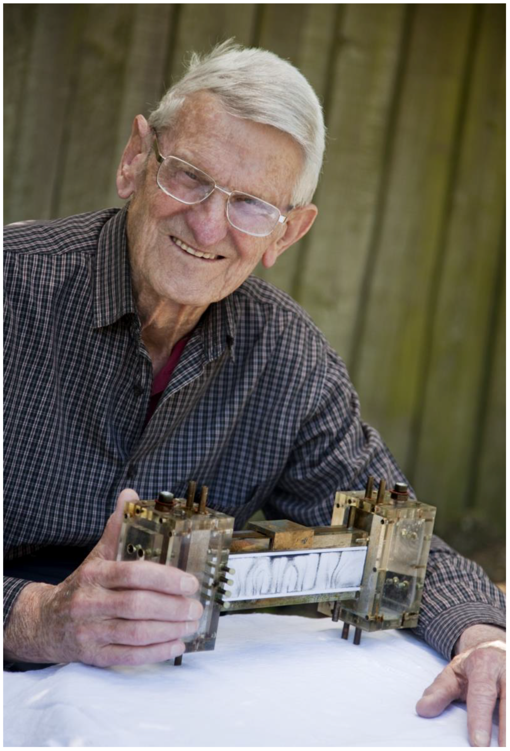
He knew of my interest in simple models of geothermal systems. One day he asked me if I was familiar with the deduction of HSJ Hele-Shaw: the flow of a viscous fluid between a pair of close parallel impermeable sheets behaves as if it were in a medium of uniform permeability. I had never heard of it. However, within the hour I had found it written up in my copy of the fluid dynamics bible (old testament, Lamb’s Hydrodynamics). Within another hour I was able to deduce, with the usual simple approximations, that the same kind of flow, as in a permeable medium, would also exist for convection in a Hele-Shaw cell.
I cannot thank Robin Wooding enough for his most fruitful query/remark.
Using such cells was to become a major part of my research. However, I did not immediately do anything with this. I got way laid. After my return, to get back into my stride, I tried a miscellany of simple convection experiments. Among these, with no clear focus I decided to see, by experiment, what I could find, by measurement and visualization, about the convective flow, laminar and turbulent, up a hot vertical wall of a container of a viscous fluid.
Perhaps nothing very new about that, just turning the handle. So I stumbled over the hitherto unknown phenomenon of a vertical stack of convective cells in what I called a “vertical slot”.
The first apparatus was the annular space between 2 concentric vertical cylinders, the inner heated, the outer of glass (from an old-fashioned petrol bowser). The motion was visualized with aluminium powder suspended in the fluid. One morning, I had set the next experiment going and at 11am went to the usual morning tea with the Cavendish mob. I returned to the lab. I got a mighty surprise. I could see it on the other side of the lab. The flow had generated a steady stack of toruses. I saw, on close inspection: the direction of the motion within the toruses was all the same.
I was hooked. In an instant, plan A dropped. I did a lot of experiments with flows in vertical slots. The numerical modelling of these flows was started later while I was at IGPP.

5.1.7. 1964–1965 Institute of Geophysics and Planetary Physics (IGPP)

Institute of Geophysics and Planetary Physics, UC San Diego at La Jolla
In the Scripps Institute I gave a graduate lecture course on geophysical/oceanographic fluid mechanics. I did a variety of convection experiments notably Hele-Shaw cell models of free convective systems of sea water within sub-ocean-ridges. [Oh, and I did a lot of surfing!]
IGPP was into computers in a very big way. For example, they had written Bullard Oglebay Munk Miller (BOMM) a super-level language (itself written in Fortran) for analysing (geophysical) time-series data recorded on digital mag-tape. When I arrived they had just wrapped up a gigantic project, based on several sites, spanning the Pacific, recording wave height, to allow tracking waves which travel right across the ocean.
So no surprise, the main new big step for me was access to quite powerful computers, initially a CDC1600 and later CDC3600—programming in Fortran, the work horse of the day. A rough-and-ready form of diagrammatic output (shown as sequences of isolated dots) was possible on the line printer output. I did several different numerical experiments, including quite an elaborate numerical study of convection in a “vertical slot”.
I cut my teeth on numerical modelling with systems of non-linear partial differential equations—being able to handle things hitherto all but impossible. For me, a door had opened into a new world.

5.1.8. 1966–1970 All Together Now: DAMTP

Department of Applied Mathematics and Theoretical Physics, Cambridge
set up and run by George Batchelor in 1959:
originally in the Old Cavendish (Free School Lane);
from 1964 in the old CUP (Silver Street); and from 2009
in the Centre for Mathematical Science (Wilberforce Road)
The new department originally combined various groups such as astrophysics and fluid mechanics.
Yet again back in Cambridge.
Busy (in the old CUP) with setting up and running the fluid mechanics laboratory with Tom Brooke-Benjamin handling the gear (2-man workshop, 1-woman darkroom/draughting, flume, rotating table, etc.) and me on measurement equipment.
I set-up and ran a hybrid-computing course for our grad students. This was with a linked digital and analogue computer, a common tool at the time. The digital computer was a Digital Equipment Corporation PDP8, one of the first mini-computers. This instrument provided a very versatile tool for controlling experimental apparatuses and handling measurements. It was also useful for experimenting with systems of non-linear ODEs. (In 1965 I had been on a 2 week full-time residential hybrid-computing course in Los Angeles, USA.)
A major project during 1969/1970 was setting up my brain-child CATAM “Computer Aided Teaching of Applied Mathematics” (original name, laterappliedchanged toall’). It ran on a TSS8, a PDP8 with 32k memory plus an additional 256k drum memory and a dual magnetic tape machine with removable reels, altogether providing a local time-shared system for 16 users on teletype machines. I started the project with 4 full-timers: 1 electronics, 1 software, 2 operators; and part-timers: a guinea-pig student and several colleagues for demonstrations and all. For its time, it was quite a pioneer.
The project is still on air, vastly changed. It plays a part in the Maths Tripos. The student work can be done with several software packages but the supported software package is MATLAB.

The Maths Lab

Before long I had another string to my bow. The Cambridge Maths lab now had ‘Titan’, a very powerful computer. The nice things, from my point of view, were: an easy-to-use programming system-and-language; but especially diagrammatic output could be written as continuous lines on a Calcomp plotter.
I became a heavy user. I was given a key to the lab. The machine was normally run as a batch processor with input via punched tape. This was OK. However, one tiny defect on the tape or a tiny programme error killed your job. However, that door key, in the midnight, gave me direct access to the machine. The operator would easily fit you in. You could see how your run was going by watching the line-printer or plotter and if bad have the operator stop the job. With just a few seconds here and there you could get done in a couple of hours what otherwise could take a week or more, and still have big runs done in batch. There was a small group of us nerdy night owls. We learned a lot from one another.
I was asked to run a course on numerical methods for PDEs for the graduate-level computer-science programme.
As part of all that, I wrote a front-end, using Titan’s standard programming language to make a sort of mini-super-level programming language, for systems of PDEs, which I called KNEES (=numerical experiments with elliptic systems). The user wrote a main programme, in this mini-super-level language, setting out the model equations, and initial and boundary conditions, more-or-less as they are written mathematically. Even a very elaborate and complex model could be defined and written on a single page often in much less than an hour. [Of course, the user could include code of the standard programming language.]

5.1.9. And Not Least We Have 1966–1967

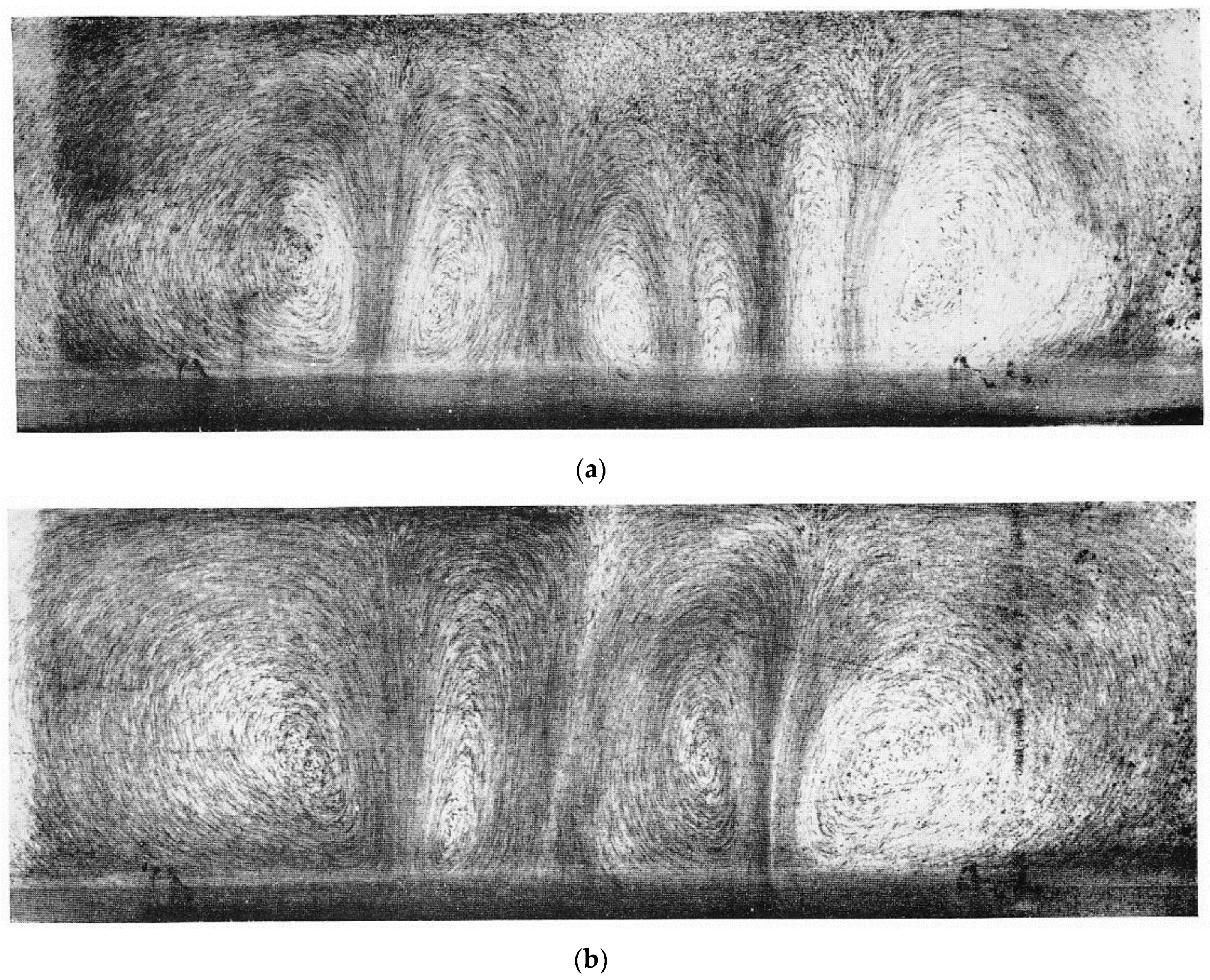
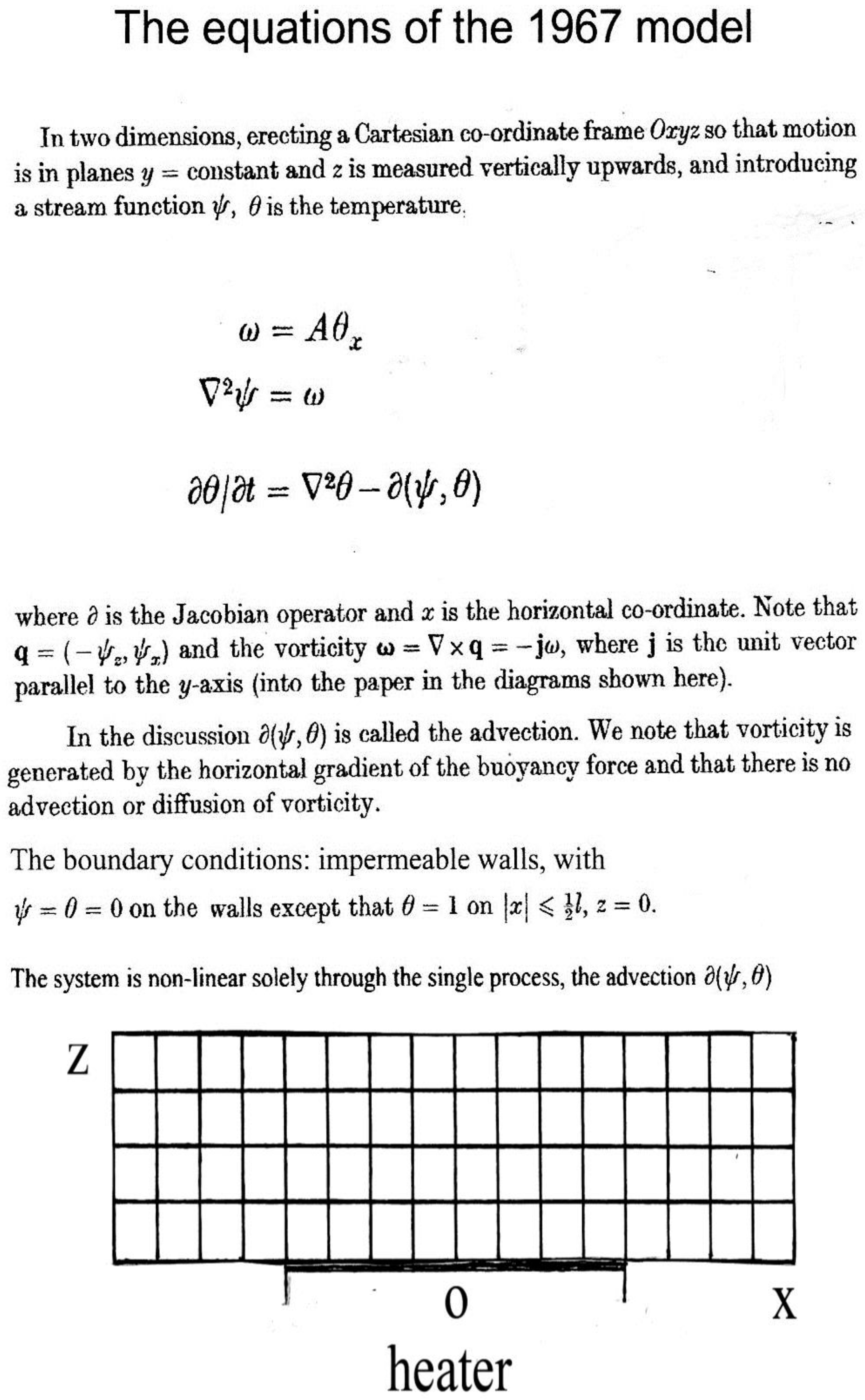
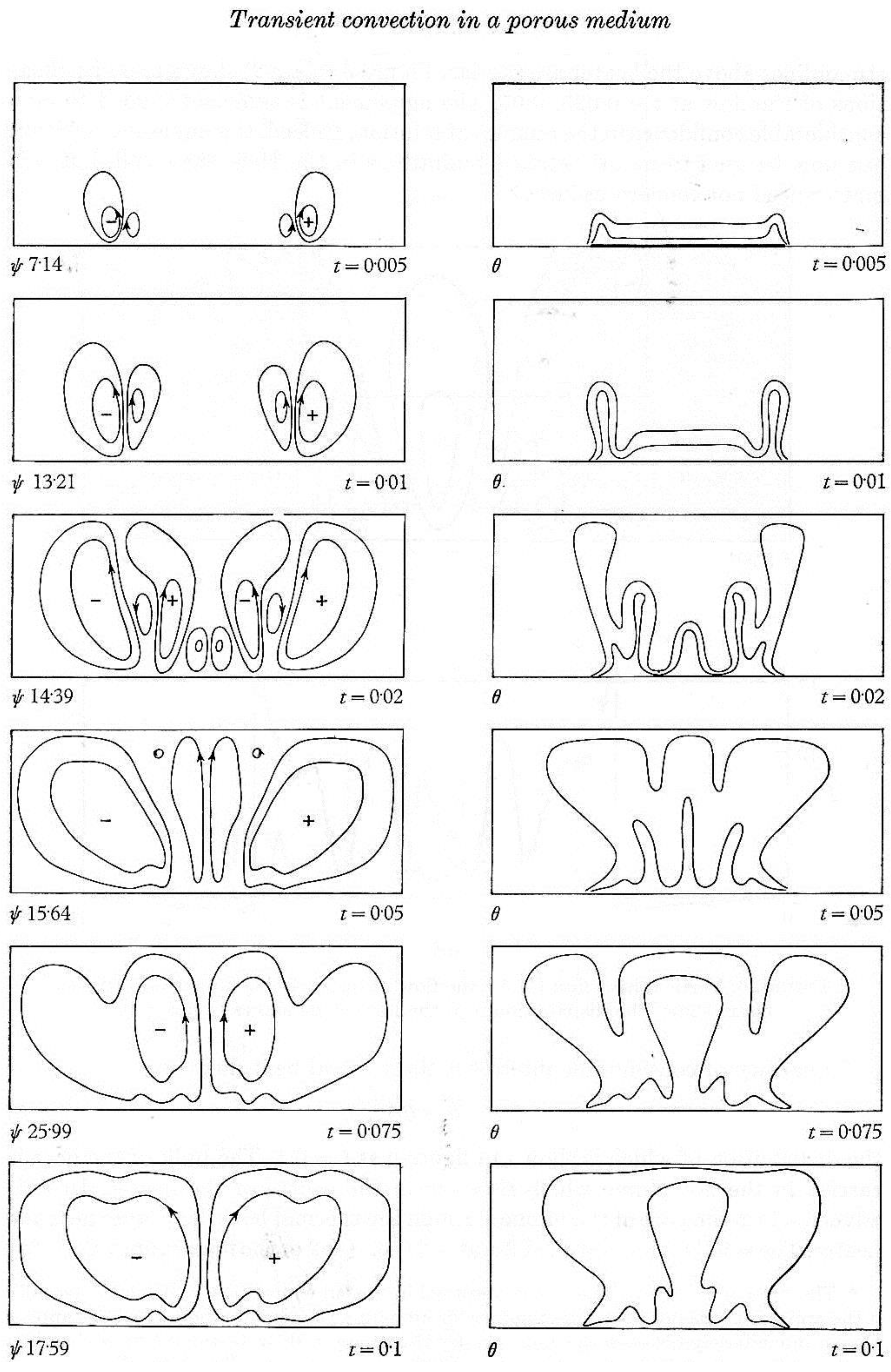
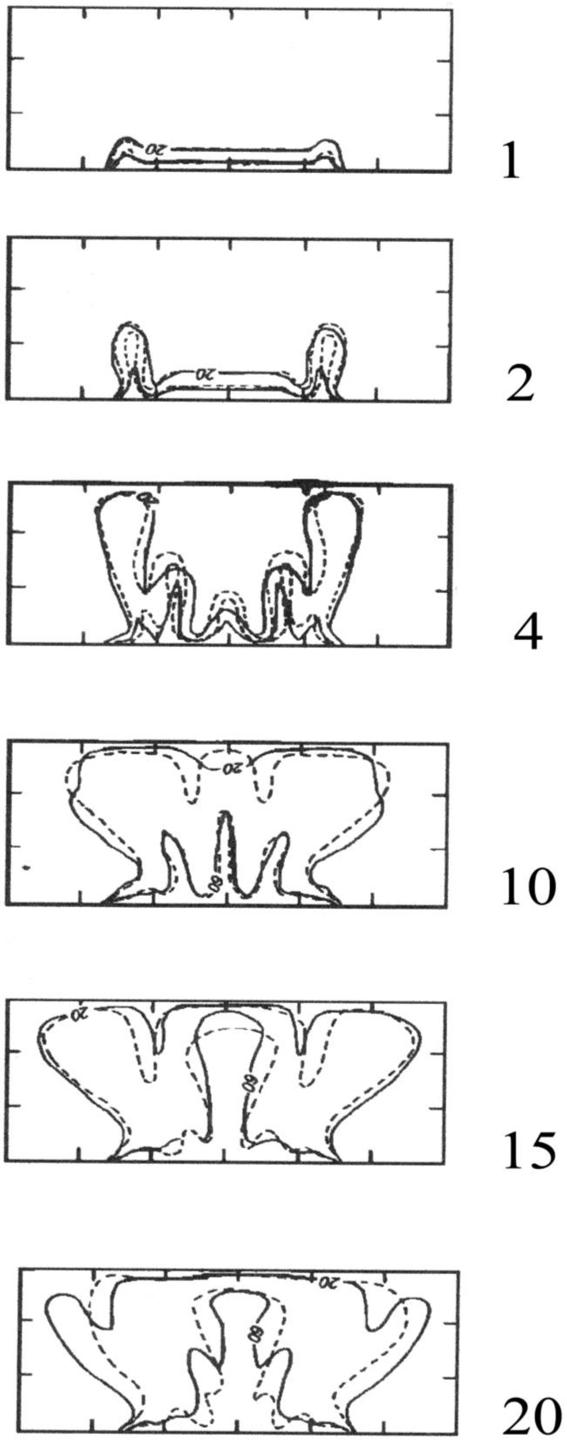
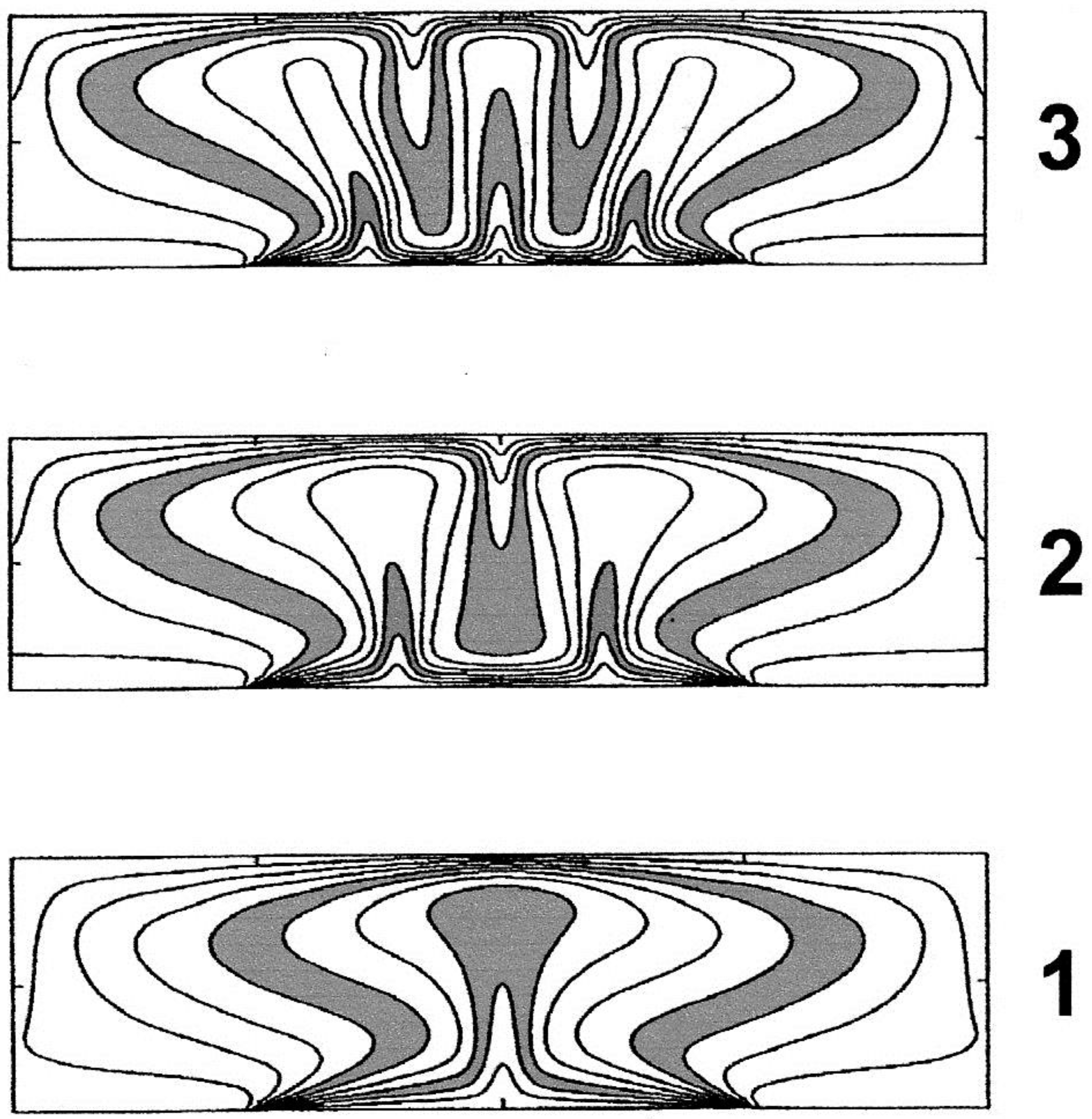
I set out to make a detailed study of free convection in a permeable medium in 2-dimensions using numerical and experimental methods. The numerical experiments were started while I was at IGPP and continued at DAMTP.
The paper (Transient convection in a porous medium. J. Fluid Mech. 1967, 27, 609–623 [2]) was focused on the comparison of the experimental observations together with simple numerical methods for both a steady state solution and the corresponding (with the same boundary conditions) numerical time-dependent solution—as much as anything to give confidence in the use of the numerical methods.
That was it!

5.2. The Model Behaviour

The model equations are given in Figure 1. The parameter A, called the Rayleigh number (often written as Ra), is a dimensionless measure of the ratio of the positive buoyancy forces to the combined negative effects of viscosity and the thermal diffusion of heat.
With A < 40, for an infinite layer and infinite heater turned on for an infinite time, there is no motion—the system is stable. The heat is transferred from the heater to the surface solely by conduction. The example here with A = 400 has vigorous convection.
Let us have a brief tour of the run as shown in Figure 2. The results are as seen in the vertical plane at various times t (in dimensionless units). On the left is the stream function. The flow develops as a set of eddies which occur in pairs: one with a clockwise motion (+) the other anti-clockwise (−).
On the right is the temperature distribution. This develops as a set of plumes (also called fingers) which transfer the thermal energy upwards. Each plume is accompanied by the upward motion between an adjacent pair of eddies.
The temperature (in dimensionless units) is initially everywhere at 0. The run begins at t = 0 when the heater is turned on by changing its temperature from 0 to 1. Heat begins to enter the fluid. For a time this is only by ordinary conduction. Away from the ends of the heater the isotherms develop parallel to the heater. However, near the ends of the heater there is a large horizontal temperature gradient and a corresponding pressure gradient. Eddy pairs immediately begin to develop (See Table 1 for plume development stages in the numerical model [2]).
Visualization of the flows in the original Hele-Shaw cell experiment [2] is shown in Figure 3.

5.3. Looking Ahead

Much of the study of this model has its motivation from practical problems involving saline fluids. The fluid density is a function of the salinity—the higher the salinity the higher the density. This is the ‘opposite’ of the case of geothermal models where the fluid density is a function of temperature—the higher the temperature the lower the density. The model equations are the same in both cases, but the boundary conditions are opposite.
The salinity version of the model is an idealization of a shallow lake of fresh water, on top of permeable ground, suddenly and thereafter continuously flooded with saline water.
  • [Set the salinity = 0 on all boundaries except for t ≥ 0, on the top boundary z = 1, from x = −l/2 to x = l/2 set the salinity = 1.
  • The container is 2l wide and 1 high.
  • The saline source occupies half of the top boundary.]
A diagram showing stream-function and temperature if turned upside down shows stream-function and salinity for the opposite dimensionless boundary and initial conditions and time.

6. Part 3: The Elder Problem Benchmark—Uptake of Elder’s 1967 JFM Paper into Modern Fluid Mechanics and Modelling in the 1980s and 1990s

The basis for the modern Elder Problem test case was the laboratory experiment published by Elder in 1967. In that original study, transient heat convection was studied in a Hele-Shaw cell heated over the central half of its base. A quarter of the way through the experiment, there were six fingers, with four narrow fingers in the centre and two larger fingers at the outer edges. Only four plumes remained at later times. Elder also presented numerical results. Interestingly, the numerical results did not agree at all well in detail with the experimental observations – though the experimental and numerical results of the gross heat transfer rate as a function of the Rayleigh number were quite good.
In the definition of the modern test case we now call the “Elder Problem”, an analogy between heat and brine transport is assumed to be valid. Hence the original physics of Elder’s experiment involving a fluid heated from below is transformed into an equivalent situation involving salt dissolution from the top boundary (OECD, 1992) [10]. Diffusion and domain length scales are scaled accordingly to maintain an effective Rayleigh number of 400 as in the original Elder Hele-Shaw cell thermal natural convection experiment. Elder’s original heat experiment is thus transformed into a salt analogue.
There are literally hundreds of papers that cite the original Elder paper or the derivative Elder Problem. To give a sense of impact of this work, a recent search (6 January 2017) found:
Web of Science: the original 1967 steady state paper has been cited 301 times; the original 1967 transient paper has been cited 212 times;
Google: “Elder Problem” AND “convection” returns about 3300 web-page hits;
Google Scholar: “Elder Problem” returns 380 relevant papers.

6.1. Key Questions

The history of the development of the Elder Problem poses some interesting questions.
(1)
How did it come into existence as the formally titled “Problem” we know today?
(2)
How did it obtain this nomenclature?
(3)
Who were the earliest scientists who studied it as a potential model code benchmark and what motivated their work?
Simply, can we trace a path between Elder’s work in the 1960s and the more familiar Elder Problem today? Providing a historical account of the very earliest uptake of Elder’s work into modern fluid mechanics and variable density modelling is of interest.
The answers to these seemingly simple, yet fundamental, questions were not clear to us. We have scoured the literature and undertaken extensive personal communication through scientific networks to try and resolve this matter as best we can from a historical perspective.
Our investigation has revealed a number of most fascinating strands to the story. It has also revealed that there were a number of key players who were instrumental in the birth of the Elder Problem as known today: Hans-Jörg Diersch, Ekkehard Holzbecher, Clifford Voss, Peter Frolkovič and Klaus Johannsen are central to this story.
We now attempt to reconstruct our understanding of the uptake as faithfully as possible. We summarise key stories, emails, discussions and information provided to us and draw some of our own insights and conclusions from those stories and the available literature.
The story of the uptake of Elder’s work begins in Germany, in both West and East Germany, at the time of the Iron Curtain’s most infamous incarnation: The Berlin Wall.
Prof. Hans Diersch worked on one side of The Wall, in East Berlin at the Institute of Mechanics of the Academy of Sciences of German Democratic Republic (GDR); Ekkehard Holzbecher worked on the other side of The Wall in West Berlin at the Technical University of Berlin.
There was no contact nor any exchanges between Diersch and Holzbecher in the years preceding the fall of the Berlin Wall. Fascinatingly, both Diersch and Holzbecher were working with and on the Elder study in their research groups – entirely independent of one another.
After the fall of The Wall (in 1990) Diersch became acquainted with Holzbecher who invited him to give a talk at his University. Diersch presented the simulation results for variable density flow which he had studied in the 1980s. During this visit and around this time, Diersch learned Holzbecher had also done simulations of variable density flow with different success (with his code FAST).

6.2. Hans-Jörg Diersch’s Story

Diersch had started his own simulations of the Elder Problem in 1980. The results were published in the Journal of Applied Mathematics and Mechanics/Zeitschrift für Angewandte Mathematik und Mechanik (ZAMM) Journal in 1981, in a paper titled ‘Primitive Variable Finite Element Solutions of Free Convective Flows in Porous Media’ [8].
This is the first paper we have found that used Elder’s work in a setting that provided the basis for a modern variable density model benchmark. The paper is published in English with the Abstract in English, German and Russian.
Diersch, worked with finite element modelling in fluid dynamics from 1973 and in porous media at the end of the 1970s. He later used the groundwater flow and transport code FEFLOW. This was released in 1979. It was designed for variable density flow because there were practical interests in saline groundwater flow. This was mostly for the lignite mining industry and salt-water upconing due to overexploitation in water stations—typical problems in the former GDR.
Diersch was looking for a method to test and verify his new code for variable density groundwater flow in porous media. He checked the literature then available and found the beginning of systematic works on unicellular and multicellular convection in porous media linked with the names Elder, Kvernvold, Schubert and Straus. These were mostly published in the Journal of Fluid Mechanics—then available in East Germany.
Diersch’s publication in ZAMM was mainly aimed at presenting the numerical details for solving free convection problems in the steady-state and transient case. In reality, these were the numerical beginnings of FEFLOW. The code name was not mentioned in the paper because the reviewers did not wish for any ‘commercial’ evidence in the final publication. In the second part of the paper, the numerical results were presented. For the transient free convection case it is said there: “To compare the finite element solutions with previous findings ... a typical model problem already investigated by Elder ... is considered”.
It is interesting that Diersch considered the case where the high density boundary (corresponding to C = 1) was located on the upper boundary. 63 finite elements (and a total number of nodes = 222) were used to simulate flow in the symmetric half domain. Three eddies were observed at T = 0.01438 and fusion of these eddies lead to one single large eddy by T = 0.02. In essence, this was then the first solute analogue to the thermal Elder Problem in the published literature. Diersch notes: “The agreement with ELDER’s results is satisfactory”.
It is clear that Diersch did not name this the “Elder Problem”. For Diersch, at that time, Elder’s work was ‘only’ one study of many within a family of cellular convection problems in porous media. He did not see a need to emphasize it against the other convection problems studied by Kvernvold and others. He also commented in a personal communication (to Craig Simmons) that he was “young and bashful” and did not feel authorized to categorize a test problem with the name of the author.
The results are described on the pages 333 to 336 of the original ZAMM paper. We can see that only the FEFLOW results are documented. Also importantly, only certain stages at earlier and subsequent times were simulated, while later times were not reached. This was because of the computational limits at that time of the available mainframe (a Soviet BESM-6 computer).
All plots were hand-made as no suitable plotters were available. Diersch hand drew all vectors. By taking the numbers printed on paper listings from line printers, the contours were redrawn from iso-line raster prints of the same line printers. Unfortunately, as one can see, there is no graphical comparison with the results obtained by Elder in the paper. There were reasons for this. First, Diersch had no way to reproduce Elder’s results in a technical format to include it in the manuscript. Second, the length of the paper was already critical. Third, the key goal of the paper was to publish results to demonstrate the ‘power’ of the new numerical methods. This was a significant achievement at the time. Diersch was quite rightly proud to publish his own new results. Elder’s results were somewhat secondary in this context and something of a means to an end, not an end in themselves.
In summary: in 1981, to demonstrate the performance of his numerical method, Diersch was the first to use the Elder Problem as a test example. It is also interesting that Diersch continued to revisit the Elder Problem at several stages, and in several papers, throughout his career. In Diersch and Kolditz (2002) he repeated the simulation in the symmetric half domain, but now this time solving the Elder Problem with grid levels for increasingly fine meshes, the finest employing 525,825 nodes for the half domain (the original ZAMM paper in 1981 had a total number of nodes = 222 for the half domain solution—so approximately a three order of magnitude increase in the number of nodes in about 20 years!).
*
Diersch and Kolditz (2002) [4] is a superb “review of the state of the art of modelling of variable-density flow and transport in porous media”. It is a ‘small book’: 46 pages and 246 references!

6.3. Ekkehard Holzbecher’s Story

In 1984, the Swedish SKI (Swedish Nuclear Power Inspectorate) initiated a co-operation between thirteen organisations from ten countries and two international organisations to “improve knowledge of the influence of various strategies for groundwater flow modelling for the safety assessment of final repositories for nuclear waste”.
The groups worked jointly setting up test cases (benchmarks) that were then treated by different groups using their modelling software. The test cases also included specifications concerning the output and presentation of results in order to enable intercomparison. Finally the results coming from the modelling teams were compared, leading to conclusions concerning the physics and set-up of the test-case or the modelling process altogether.
The first project of this type was INTRACOIN, focusing on models for radioactive decay, followed up by HYDROCOIN, dealing with “groundwater flow modelling for the safety assessment of final repositories for nuclear waste”. Going through three subsequent levels of modelling (testing, validation, sensitivity analysis), the final report appeared in 1992 (OECD 1992) [10].
Holzbecher’s work with the Elder Problem began as part of the HYDROCOIN project. In 1984 he joined a project group at the Technical University Berlin (TUB), headed by Eckart Bütow, that dealt with modelling for safety of repositories for high level nuclear waste. The aim was to study potential sub-surface flowpaths from the disposal site within a saltdome towards the ground surface. The project was part of a bigger research conglomerate called PSE (Projekt Studien Endlagerung) and worked on studies for several real sites in Germany. As a mathematician Holzbecher was responsible for the software (SWIFT) and also for the participation within the HYDROCOIN project. (The SWIFT code performed quite badly on the at that time new CRAY computer installed in West-Berlin.)
Eckart Bütow and Ekkehard Holzbecher were participants at all the HYDROCOIN meetings at that time. Eckart Bütow was the one who guided participation in HYDROCOIN. The decision to be the pilot-team for the salt problem cases, was nearby, as Germany was the country which favoured the storage of waste in salt formations (salt-dome option) most of all involved countries, at that time. The development from the Saltdome testcase (level 1) to the Elder experiment (level 2) back to the Saltdome (level 3) was also a result of discussions within the HYDROCOIN meetings. Bütow encouraged Holzbecher to keep working in the direction that had been discussed, and gave Holzbecher the opportunity to do so within the Berlin team.
The first salt test problem was (HYDROCOIN level 1 case 5), now referred to as the ‘Saltdome-Problem’. Many doubted whether the solutions, to the Salt-dome test case, calculated by numerical simulations, were physically sound. That became apparent during the HYDROCOIN meeting at the OECD offices at the end of 1984. The final report noted: “Initial results … varied considerably between the different Project groups. The cases proved to be very complex with the presence of both free and forced convection. Convection cells appeared within the flow domain”. (OECD, 1992) [10].
At a HYDROCOIN meeting in Paris the British group mentioned an experiment in which eddies were observed. They recommended Holzbecher look into it. The British group lead by David Hodgekinson, including Alan Herbert (see for example, Water Resources Research, 1988), were concerned about the thermal effects of nuclear waste disposal. In their literature review they had found Elder’s experiment. With this limited information, back in Berlin, there it was in the Journal of Fluid Mechanics in the Mathematics library just 3 floors below Holzbecher’s office. Holzbecher started to look in more detail into several of John Elder’s publications in JFM, and the references therein, especially R. Wooding’s publications. After a while (the exact time is uncertain) Holzbecher learnt about Hans-Jörg Diersch’s publication. The journal ZAMM was also available in the same library.
So, while The Wall was still standing, Holzbecher knew that there was someone (maybe a team) working in a similar way as they did, on the other side of the same city. Of course they would have liked to make contact, at least, but how? Officially there was no co-operation between the scientific organisations of both German states. They did not know any exact coordinates of the people on the other side of The Wall in East-Berlin. Taking any initiative from their side, if successful, could even have been dangerous for the East-Germans. In the GDR ‘west-contacts’ were suspicious. So, there were two Elder Problem hot spots without connection in the very same city, obviously! But any connection between those activities was forbidden.
Holzbecher proposed the Elder experiment as a test case in level 2 (following a hint from the British as mentioned earlier). After two years, in autumn 1986, Holzbecher quit the waste disposal project and started working as an Assistant Professor at the same university. His office just moved one floor below in the same building. Holzbecher was even nearer to the Mathematics library, which he happened to frequent equally often, as he had decided to take the topic of ‘density-driven flow’ to his new job. Holzbecher stayed in contact with his former colleagues, working one floor above, but that project survived less than one year longer.
Interestingly, Holzbecher proposed the Elder test-case as what was thought to be a simpler test-case. The OECD report [10] notes “The present test case (HYDROCOIN level 2 case 2) which represents a less complex problem involving only free convection, was proposed to study the behaviour of the convection cells in detail. The basis for the case was a laboratory experiment published by Elder in 1967”. (In discussions participants usually referred to the ‘Elder test-case’.)
Elder’s original experiment heated the fluid from below. In order to connect the HYDROCOIN work with its salt interests, Holzbecher transformed the Elder thermal set-up into a saline problem with salt dissolution at the top.
Within the HYDROCOIN project many groups had solutions for the Elder test-case, among them: METROPOL from the Dutch group; NAMMU from the British; CFEST from the US; and SWIFT from the German group. For the first simulation period with the onset of convection very similar solutions were observed. All groups had convection cells (eddies), confirming that different flow patterns appear if density effects are taken into account: instead of a moving diffusive front one obtains convection cells. This was the major conclusion taken by the HYDROCOIN project, concerning the Elder test case.
The Elder test-case became part of Holzbecher’s doctorate thesis (1991 in German in Civil Engineering at TUB) [11]. For modelling he used the commercial SWIFT (1982) code and his self-developed FAST-C(2D) code. Both codes used the finite difference method. For transient simulations an implicit time-stepping method was used (in contrast to Elder). Flow and transport were coupled by a so-called Picard iteration. Using FAST with vectorized solvers for the linear systems the execution time for solving the Elder Problem was reduced by a factor of 40 in comparison to the SWIFT model. In his thesis there is a comparison of four codes: SWIFT, FAST-C(2D), SUTRA (provided by Voss) and Elder.
Holzbecher compared temperature and corresponding salinity contours at selected time instants. He also compared stream function maxima and Nusselt numbers published by Elder with FAST-C(2D) outcomes for two meshes of different grid spacing. Results deviated by less than 10%. Higher deviations were observed between results of SWIFT and FAST-C(2D) for high Ra = 400 and long simulation times. The final flow pattern showed two convection cells in the complete system.
After The Wall came down, the curtain gradually was lifted. It was an exciting time, but it took some time for both sides to open. As far as Holzbecher remembers, he met Hans-Jörg in person in 1991 at a conference, not in Berlin, but in Tallinn, Estonia. They had some very nice talks together and he enjoyed sharing their experiences about groundwater modeling, numerical algorithms and solvers, and so on. As far as Holzbecher can remember, he and Hans-Jörg Diersch did not talk about the Elder Problem.
Around the same time together with another East-Berlin scientist Holzbecher had started to organize a ‘colloquium’ that took place at Technical University Berlin every Friday during the semester. The idea was to bring together people from the former East and West to present their findings for an audience, which was also partially from East and West. This colloquium endured for several years and was always well frequented. On one of these Friday afternoons, probably in the winter semester 1991/1992, Hans-Jörg Diersch was invited and gave a presentation about his work with FEFLOW and he mentioned his simulations of the Elder experiment.
Holzbecher continued working on the topic of density-driven flow, and in 1998 published the book Modeling Density-Driven Flow in Porous Media [12], which was also his habilitation thesis at Freie Universität Berlin (FUB). Several benchmark problems are tackled in the book: the Henry Problem on saltwater intrusion; 2D Bénard convection; the Saltdome Problem; and the Elder Problem. Using the dimensionless approach implemented in FAST-C(2D) he explored solutions for the thermal problem and compared them with Elder’s results. For coarse mesh sizes the system converges to a two cell solution (i.e., one cell on each side of the entire system), while for refined meshes (160 × 80 for the half system) the final solution shows 4 cells. In the book chapter on the Elder Problem a review is given for solutions obtained by other codes before and after HYDROCOIN.
In 2005 Holzbecher published a paper benchmarking the commercial FEMLAB code for variable density test cases. Upgraded versions of this Finite Element code are nowadays known as COMSOL Multiphysics. Using quadratic elements on triangular meshes, again a dependence on mesh refinement was discovered: for a mesh of 8240 elements, the simulation converged to a 2 cell flow; while other mesh sizes gave a 4 cell flow (Holzbecher 2005) [13].
Since then Holzbecher has further explored the COMSOL code. The code offers options for using: different differential equations (primitive variables rather than the dimensionless approach); different finite elements; different mesh types; different solvers; etc. In most recent simulations: temperature dependent thermal properties (density, viscosity, thermal conductivity and heat capacity) are taken into account.

6.4. Cliff Voss’ Story

Voss and Souza’s (1987) [9] work considered the Elder Problem as a test case for verifying variable density flow models using the SUTRA (Saturated-Unsaturated Transport) code.
They state: “The authors gratefully acknowledge … and the research group headed by E. Buetow, Technical University of Berlin, for suggesting the Elder problem as a test case”.
Voss, himself involved in the HYDROCOIN project, recalls that Bütow and Holzbecher suggested the Elder Problem to the HYDROCOIN group. Voss met Bütow and Holzbecher in the 1990s as part of that project.
It is clear, however, that HYDROCOIN only ever refers to “test cases” and never to “problems”.
Following its introduction as a HYDROCOIN test case, Voss and others tried it. Voss and Souza (1987) remark: “The numerical results of Elder [1967] for a problem of complex natural convection are further suggested as a basis for verification of transport simulators. The primary value of this test is to verify the accuracy of a simulator in representing bulk fluid flow driven purely by fluid density differences”.
With their SUTRA code, they simulated the solute analogue of the model in Elder (1967) [2]. See Figure 4 which shows Figure 9a from the original Voss and Souza (1987) [9] paper. Here, we turn the figures upside down to allow easy comparison with the thermal original. Voss and Souza (1987) [9] give the time in nominal years: 1 year = 0.005 dimensionless time. The SUTRA results are shown in solid lines. The Elder (1967) [2] results are shown in dashed lines.
Though they used a much coarser grid (of 1170 nodes versus 3200), the detailed agreement is quite good. Their code and the benchmark mutually supported each other!
Comparing Diersch’s ZAMM paper (1981) [8] with that by Voss and Souza (1987) [9], it is clear the latter focussed on the Elder Problem in more detail. They published it in a more mainstream journal which is widely read by the water resources community.
Voss and Souza refer to the “Elder problem”—the first such use we could find of this nomenclature in written literature. [But we do not know who, where or when (ca. 1980?) the name was first used.]

7. Part 4: Quandary and Resolution—Late 1990s and Early 2000s

7.1. The Quandary

There was much discussion in the literature, at conferences and casually, about the many codes employed to solve the Elder Problem and the divergence among the various results that were obtained.
A key issue was the number of plumes or fingers and the nature of the central down-welling and up-welling. Among the various codes, these big differences, seemed to depend on: the role of grid spacing; different numerical solutions; and formulation of governing equations.
Early insights are in fact to be found in the OECD (1992) report [10]. There is good agreement between model results and the original Elder study. The report states “The results at the time of 1 year show very modest development of the stream-function for the reported results, while at 4 years, in all the calculations, a total number of six cells of different sizes are present. This is in agreement with Elder’s experimental photograph. At 10 years four cells are present, also in conformity with Elder”.
Yet in the immediate following sentence we read that the very first teams working on the Elder test case observed different solutions that were apparently grid dependent: it is reported “A finer grid giving smoother curves and removing a pair of eddies at the base of the domain”.
The historical and scientific significance of this observation—stated in a single simple sentence—can hardly be overstated. Some divergence amongst the results from the teams were stated as plain observations but without follow up analysis or resolution. Critically, however, the original HYDROCOIN team had already observed the key issue that would plague scientists for some 30 years.
There were clearly other limiting methodological challenges. The early OECD analysis [10] noted: “The form in which the experimental data were represented in the original report (Elder 1967) did not allow a quantitative comparison between the calculations and the experiment. Instead, two photographs of the convection cells, published in the experimental report, could be used for qualitative judgement of the results of the validation exercise … In addition to a set of dimensionless parameters chosen by Elder for both the laboratory and numerical experiment, a set of physical input parameters were supplied, which matched the dimensionless parameters used by Elder but for an enlarged model domain. The output was restricted to a qualitative comparison of the results of numerical models with that of the laboratory experiment for stream-function and concentration distributions at six different times”. The matching exercise was limited to a qualitative comparison at best and the limitations were pointed out by the authors of the report.
With the benefit of hindsight: the “less complex problem involving only free convection” (OECD, 1992) [10] afforded by Elder’s work was not less complex at all!

7.2. The Resolution

Our story is one of a gradual awareness, during the 1980s and 90s, of the unexpected behaviour of the model—with numerous different numerical solutions. How it slowly and hesitatingly dawned on the explorers of the model: there might be more to the quandary than mesh spacing; not just difficulties with the numerical codes.
Early on, being preoccupied with the expectation of a single steady system, there was much worrying about whether or not the central plume should be up-welling or down-welling as found with different numerical methods.
To cut a very long story short: it was slowly realized there might be more than one stable state; and ultimately other different steady-state solutions were identified numerically.

7.3. Peter Frolkovič’s Story

Frolkovič and De Schepper (2001) [3] found 3 stable steady-state cases
Frolkovič got a postdoc position in Erlangen (Germany) in 1995 to participate on a large scientific project involving five different universities (the same large R&D project dealing with the risk assessment of nuclear waste disposal noted in Johannsen’s story). He was cooperating among others with Klaus Johannsen from University of Heidelberg and Carsten Schwarz from ETH Zürich on that project. The most important output of the project (finished in 1998) was the software tool called d3f (distributed density driven flow) to simulate variable density groundwater flow in 3D using parallel computations.
Frolkovič was responsible for discretization methods in the project. An important part of the development was testing the code and the Elder Problem was a very clear choice to solve. There were some open questions and surprises related to this problem discussed several times between Frolkovič, Johannsen and Schwarz. Comparing incompatible numerical results obtained by d3f a question arose if more than one stable steady solution of Elder Problem exists.
Indeed, using d3f it was possible to find three stable steady solutions. [The same three solutions have also been found by other authors using different models. The three stable steady solutions for the Elder Problem are shown in Figure 5.] Such results were for the first time reported by Schwarz in 1997 and published later in his PhD thesis Dichteabhängige Strömungen in homogenen und heterogenen porösen Medien that was submitted in 1999 at ETH Zürich. According to Schwarz in his words “the Elder’s experiment and the corresponding simulation was an ever-present notion during my doctoral thesis”. Schwarz left the academic community after finishing his PhD thesis and has worked at UBS Bank since 1999.
Frolkovič left Erlangen in 1998 and moved for one year to Ghent in Belgium. This stay was not related to d3f, but he found time to continue on the results from the previous project. Together with his colleague Hennie De Schepper he was interested on the development of upwind methods for convection dominated transport coupled with variable density flow. The Elder Problem was a perfect example to show advantages of such methods. To publish related numerical simulations it was obvious to try also to explain the seemingly incompatible results published by various researchers for this problem.
The work was finished and submitted by Frolkovič and De Schepper in July 1999 without knowledge of PhD thesis of Carsten Schwarz. In this paper [3] (published online in 2000 and printed in 2001) three stationary solutions are reported together with the settings for transient simulations to obtain them.
According to Frolkovič and De Schepper [3] and opposite to previous published works the numerical solution of Elder Problem on the finest computational grid is reported to have at later times only one finger. Although it was shown that some small perturbations in input data or in numerical approximations can cause different behaviour of transient numerical solution of the Elder Problem, it was claimed in this paper that the one finger numerical solution should be considered to be free of such perturbations.
*
There are two important observations that can be made at this point in the historical evolution of the Elder Problem. Firstly, only stable steady state S1 was observed in Elder’s classical JFM 1967 paper. Secondly, whilst Frolkovič and De Schepper (2001) [3] report 3 stable steady-state cases they made no attempt to quantify the bifurcation diagram and to determine the existence of these three stable steady-states for different Rayleigh numbers. This would, however, soon be the subject of work by Johannsen (2002, 2003) [5,6] and then later van Reeuwijk et al. (2009) [7].

7.4. Klaus Johannsen’s Story

Johannsen (2002) [5] found 11 steady-state cases: 3 stable plus 8 unstable; and which showed (Johannsen, 2003) [6] the same behaviour for the stable steady-state cases with or without the Boussinesq approximation.
In 1992 Johannsen joined the group of Gabriel Wittum at the University of Heidelberg and in 1995 he led a large R&D project dealing with the risk assessment of nuclear waste disposal in salt formations. This way Johannsen got in contact with the density-driven flow community: he worked together with P. Frolkovič in Erlangen and with Wolfgang Kinzelbach and Carsten Schwarz at the ETH Zürich. Johannsen got to know the work of Diersch, Voss and Souza, Simmons, Elder, Holzbecher, Kolditz and more.
The Elder Problem was chosen to be one of the benchmark problems. Initially, it seemed to be a rather simple one. Only, there was quite some confusion about what the ‘true’ solution of the problem would be, as frequently two very different solutions were observed. The first step to solve that problem was given by Frolkovič and De Schepper (2001) [3]: they found that 3 steady-state solutions existed. Being quite bold, Johannsen said to himself: Let’s solve this problem once and forever, so that we can discuss something different. Johannsen had the chance to carry out high resolution simulations on massively parallel computers—and he used them. What turned out was that there are in fact several steady-state solutions to the Elder Problem, as Frolkovič and De Schepper [3] discovered, and depending on the perturbations of the discretization schemes (time and space), one would see the one or the other appearing in numerical simulations. Elder’s initial conditions are so close to the border of the basins of attraction of the two solutions, that the whole transient simulation of the Elder Problem was extremely sensitive to perturbations. In personal correspondence with Craig Simmons, Johannsen noted his conclusion: “It is not interesting to know, what the correct solution to the Elder Problem is. It is either the one or the two finger solution. You would know if you refine your grids enough. If your software is producing the right solution on a coarse grid, this is not necessarily because of quality, but might be chance”.
So Johannsen thought it better to spend time to understand the solution structure of the Elder Problem. That led him to the study of dynamical systems and bifurcation analysis. Johannsen programmed that and applied it to the Elder Problem. He found 3 stable steady-state solutions (much along the lines Frolkovič and De Schepper [3]).
Johannsen got excited and found more and more, this time 8 unstable steady states, that had not previously been documented in the literature: every second day he would run over to Peter Frolkovič, who was at that time his colleague in the group of Wittum, to tell him: “I got a new one”.
Johannsen (2002) [5] noted that: “The stable solutions s1, s2, s3 can be found by a transient simulation. s1, s2 frequently occur in the simulation of the Elder problem. Solution s3 can be found by choosing appropriate initial conditions”. Further, “For (300 < Ra), e.g., for the original Elder problem (Ra ≡ 400) we have (at least) eleven solutions (three stable, eight unstable)”.
Then Johannsen started to compare the Boussinesq with the non-Boussinesq approximation (Johannsen, 2003) [6] and the associated bifurcation diagrams—with similar results for the stable steady-state solutions, but a significant difference for the unstable steady states. He concluded that further investigations on this matter were necessary.
At the end Johannsen concluded: a seemingly simple problem turned out to be a very complex one.
*
By then we were certainly set in concrete! [If there are other distinct stable-unstable states, as yet, is not known.]

7.5. Craig Simmons’ Story

Craig was invited to give a keynote address: Variable density groundwater flow: From modelling to applications at the UNESCO Water and Development Information workshop: Arid Lands: Hydrology Modelling. This was held in Lanzhou, China, 11–15 June 2007.
He discussed the Elder Problem and the quandary of multiple solutions.
There followed vigorous discussion regarding variable density flow and solute transport with general agreement that these unstable fluid problems are challenging.
Over lunch, Simmons was approached by Simon Mathias (then with Imperial College London). Mathias was unknown to Simmons. Simmons had no idea this encounter would be the start of something big. They chatted about Simmons’ talk.
Then Mathias said: ‘In a rather different field we have used a very good method called the pseudospectral method. It is quite different from the usual finite difference methods. Perhaps you should try it’.
He remarked that we should be able to do better than with our current numerical simulators by using this method. Mathias explained how it worked and how he had been using it. He said by using it we could eliminate numerical noise and get numerically uncontaminated insights into the physics of the problem. Simmons was intrigued. He was very excited. He would need to follow this up! Their parting words at the conference were that they would commit to working together on the Elder Problem using the pseudospectral method. Several weeks later by email they started to discuss how they might do it. Simon Mathias and Craig Simmons worked with Maarten van Reeuwijk and together they began the journey.
A benchmark needs to be reliable and not clouded in uncertainties. To see if the Elder Problem does not suffer from these uncertainties, van Reeuwijk, Mathias, Simmons and Ward (2009) [7] employed the pseudospectral method particularly to avoid numerical error associated with mesh spacing. Results confirmed that multiple steady states (rather than numerically spurious states) are indeed real - intrinsic characteristics of the Elder Problem. van Reeuwijk et al. (2009) [7] produced the bifurcation diagram for the Elder Problem for 0 < Ra < 400 by plotting Sherwood number (Sh) versus Rayleigh number (Ra). They observed: “The only solution which exists for the entire range of Ra is S1. From Ra = 76 onwards, S2 comes into existence via a fold bifurcation. Similarly, S3 comes into existence at Ra = 172”. They also noted: “An interesting detail is that near the bifurcation points, Sh for S2 and S3 is lower than for S1. Sufficiently far away from the bifurcation points, solutions with more plumes have a higher Sh. The bifurcation points are comparable with Johannsen (2003) who reports that S2 and S3 come into existence at Ra = 67 and Ra = 151, respectively. The slight differences are most likely caused by the different numerical methods”.
We were then in reinforced concrete!
An aside. With hindsight, we should not have been surprised by the behaviour of the benchmark model. We have known for many years the complex nature of non-linear systems with several possible modes.
Different model codes being tested with the Elder Problem will usually yield at least one of the three possible steady bifurcation solutions. All of these states are real, valid and acceptable.
As a benchmark the Elder Problem can be used in several ways.
The simplest and most straightforward is to select a sufficiently low Rayleigh number to get a single bifurcation state and hence a single solution. A choice of Ra = 60 is recommended by van Reeuwijk et al. (2009) [7].
A much more demanding test is available by selecting a higher Rayleigh number, Ra > 200 (perhaps Ra = 400 as in the original model).
We learned a lot through the journey. Some of it was strategic, most of it serendipitous. With hindsight, we now see that van Reeuwijk and colleagues’ work was building very nicely on the work and insights already found by Frolkovič and De Schepper [3] and then Johannsen [5,6]. The history of the work, as we lived it, could be written as if the work proceeded in an orderly way, strategic and well considered. Yet, it did not unfold in that way at all!
The use of the pseudospectral method really helped to quantify the bifurcation states using an independent method, and in a numerically uncontaminated environment. These multiple lines of evidence, from different authors using different methods, made the case and verdict for the Elder Problem plain, unequivocal, and compelling—these three stable bifurcation states were physically plausible and not numerically spurious artefacts of the numerical simulation.

8. Epilogue

Our story began with Elder’s Hele-Shaw cell experiments and numerical simulations in Cambridge in the 1960s published in Journal of Fluid Mechanics (1967) [1,2]. Through the 1980s and 1990s, this pioneering work went on to become the basis for the classic Elder Problem benchmark for numerical models of variable density flow we know today. In the 1990s, the perplexing discovery was made that different numerical models gave different answers to the same test case problem, seemingly numerically spurious artefacts of the models themselves. Finally, there was a breakthrough. In the late 1990s and early 2000s it was discovered that multiple bifurcation states are intrinsically physically realistic solutions to the Elder Problem—three stable bifurcation states are physically plausible and not numerically spurious artefacts of the numerical simulation. We had finally reached a scientific consensus on a difficult problem. In some ways, it felt like we had reached scientific nirvana. In retrospect it may all seem rather obvious and easy. Fascinatingly, the earliest clues in this scientific detective story were there in the 1992 OECD HYDROCOIN Report [10]. It took time, but we got there!
Elder’s pioneering experiments in Cambridge some 50 years ago took on a life of their own.
In recent years, a large body of work has been spawned by or underpinned by the Elder Problem. Amongst many others, these studies include dense plume migration in heterogeneous porous media (e.g., Prasad and Simmons, 2003, in Water Resources Research) and studies of reactive transport phenomena in variable density flow (Post and Prommer, 2007, in Water Resources Research). We wait with curiosity to see what other work evolves from Elder’s classic study and the Elder Problem Benchmark in the future. However, there are perhaps immediate and obvious needs that can be articulated today. The goal of our present paper was not to produce a comprehensive review of the field of density driven flows, but rather a focussed historical autobiographical and biographical memoir of the scientists involved in the story of establishing and solving the Elder Problem. However, as we prepared this paper, a more general observation was made. This observation is also in keeping with the spirit of Elder Problem history. We believe it would be nice but also important to work towards a generally accepted consensus on the reliability of mathematical and numerical modelling for variable density processes in the subsurface. Here we think not only the Elder Problem, but others such as the Saltdome Problem, the Saltpool Problem or the Salt Lake Problem, and the simulation of density driven flow and transport processes more generally. This observation was made as we reminisced about the Elder Problem and it reminded us of the unresolved issues and remaining challenges in the modelling of density driven flows more generally. It is also prompted by recent and promising advances in computational and numerical matters such as high resolution (semi-) implicit schemes for advection dominated problems. There appear to be demanding, interesting and important and as yet unresolved areas ripe for research investigation in the simulation of variable density flows.
As we write the very final words of this paper and reflect on a 50 year journey, we are struck forcefully by a number of matters. For example, where can you find, for a 2-dimensional time-dependent system, a simpler set of equations with a single dimensionless parameter and a single non-linearity?! Who would have ever realized what lurked in those very simple equations: such elaborate flow structures; the multiple steady states; the complex continuously near-stable-unstable states?! What wonderful complexity of such an at-first-sight simple system. Quite, quite fascinating!
And a powerful lesson: how to decide the possible validity in the real world of elaborate numerical models with many non-linearities and many dimensionless parameters.
And an excellent example: how we scientists fumble our way to new discoveries.
*

9. Additional Remarks

As a scientific memoir and not a scientific review, our paper deliberately focusses on the Elder Problem benchmark and we quote only the papers directly related to our story. It is not a comprehensive review of papers pertaining to the Elder Problem, nor to other similar or related free convection in porous media problems. Cellular convection problems (of porous media) in general are beyond the scope of the current paper. The reader is referred to the book Convection in Porous Media by Nield and Bejan (1992, 1999, 2006, 2013 and 2017) for an exhaustive review of the topic of convection in porous media.
It is interesting to note, however, that there is a connection between the Elder Problem and the classical, well-studied Horton-Rogers-Lapwood (HRL) Problem. The HRL Problem was first examined by Horton and Rogers (1945) and independently by Lapwood (1948). The HRL Problem is a porous medium analogue of Rayleigh-Bénard convection (natural convection in a horizontal layer of fluid heated from below). Rayleigh-Bénard convection (and its porous medium HRL analogue) are amongst the most commonly studied convection phenomena because they can be readily studied experimentally and have analytical solutions. Elder was familiar with this early work. He referred to it in his DSIR Bulletin 169 of 1966 (written during 1961/1962 mostly about work done in 1956 and 1959–1961). Importantly, this early work focussed mostly on the onset of instability. Elder knew about the critical Rayleigh number for the onset of instability Rac = 4π2 for the HRL Problem. He had even met Ernest Ralph Lapwood (known as Ralph) during his first time in Cambridge. Elder’s work was preoccupied with finding what happened to the convective system at the highest possible Rayleigh number he could get in the laboratory or on the computer—to compare with the natural systems. The earliest work by others which stimulated Elder most was that in Iceland by T. Einarsson (1942), G. Bodvarsson (various papers 1948–1961) and Italy (Larderello) by F. Penta 1954, R. Burgassi 1961, R. Burgassi (et al.) 1961.
For the classical Elder Problem two aspect ratios are given specific values. In terms of domain height H, domain width W and heated length L the values of these two aspect ratios are W/H = 2, W/L = 2. We note that for W/L → 1 the (then generalized) Elder Problem transforms into the HRL Problem and that there is therefore a connection between the Elder Problem and the HRL Problem. We further intuit that the number and nature of stable states may depend strongly on the values of W/H and W/L. In an interesting side note, John Elder explained that he had done many computer runs for a wide range of (W, H, L) with and without random ‘noise’ in the temperature of the heater. He also did laboratory models with several different geometries. At the time of writing up his work in 1967, Elder quite arbitrarily chose the parameters (for his JFM paper) as a set which in his view gave a good representative example of the behaviour of the numerical model. The remainder were not published. To the best of our knowledge, the dependencies between the number and nature of the stable states and the two aspect ratios W/H and W/L have not been formally investigated in published literature and would be an interesting topic for future research. Furthermore, the Elder Problem benchmark is concerned with stable convection states. The behaviour of the non-steady states (see Johannsen, 2002 and 2003) [5,6] and their dependency on the two aspect ratios would also be an interesting study for future research.
The HRL Problem (treated as a porous medium analogue of Rayleigh-Bénard convection) has also been used as a model benchmark by several authors. A major difference when using the Rayleigh-Bénard (HRL) Problem or Elder Problem as a benchmark is, that in the former case one compares model results with a known analytical solution as an accepted reference. For the Elder experiment we do not have a reference analytical solution. Accordingly, we can only rely on the intercomparison of results obtained from different numerical models.

Acknowledgments

Craig T. Simmons and John W. Elder gratefully acknowledge discussions and personal written correspondence with and materials provided by Hans-Jörg Diersch, Peter Frolkovič, Ekkehard Holzbecher, Klaus Johannsen and Cliff Voss that lead to and afforded this history of the Elder Problem. We are grateful for their honesty, patience and perseverance as we wrote this story.
We would like to sincerely thank Clifford Voss for providing detailed written correspondence that directly formed the basis for his story in our paper, for reviewing and checking his story in the final version of our paper, and for factual verification and confirmation of its historical veracity. This is most important for the historical record. We thank Clifford Voss for his most helpful and constructive contributions to this paper and for his important role in establishing the Elder Problem benchmark.
Craig T. Simmons and John W. Elder especially remember Robin Wooding.
We thank Jo Wooding for passing on Craig T. Simmons’ email to John W. Elder all those years ago and for introducing us.
Craig T. Simmons and John W. Elder especially acknowledge the support and help we have received from our respective partners, Brodie and Lynley.
We thank two anonymous reviewers for their helpful reviews of this paper. We thank the Editors of the Special Issue of Fluids on Convective Instability in Porous Media (Antonio Barletta and D. Andrew S. Rees) for the invitation to write for the Special Issue and their support and encouragement of this somewhat non-traditional paper.
We have endeavoured to do our very best to remain faithful to the story and to capture all the personal and scientific reflections shared with us by our colleagues. As is the case with many historical works, some elements of the story remain incomplete or unknown. They may never be known. With the passing of time, some elements of the story become vague and rely on distant memories or second hand anecdotes. We have worked hard to gather information from primary sources and to check all sources of information—and double check them. We have avoided every temptation to invent history. Where something is not known, we have simply said so.

Author Contributions

The paper itself was composed jointly by Craig T. Simmons and John W. Elder with extensive written contributions from all authors of the paper.

Conflicts of Interest

The authors declare no conflict of interest.

Appendix

Protagonist CVs
Figure A1. John W. Elder with the actual Hele-Shaw cell apparatus he used for his experiments at Cambridge in 1967 (Photo taken 5 January 2017).
Fluids 02 00011 g006
John W. Elder, born in New Zealand (1933), is an ex-academic geophysicist known for his studies of the dynamic role of the interior heat of the Earth. He obtained MSc degrees in mathematics and in physics at Canterbury University College in Christchurch (1951–1955) and a PhD degree for studies in fluid mechanics at the Cavendish Laboratory in Cambridge (1956–1958).
He has worked professionally mostly in England at Cambridge and Manchester, but also from time to time in California, Greenland, Iraq, Italy, Japan, New Zealand, Switzerland and Turkey. Since 1984 John has been Professor Emeritus (Geophysics, University of Manchester).
Fluids 02 00011 g013
Figure A2. Craig T. Simmons.
Fluids 02 00011 g007
Professor Craig T. Simmons FTSE is a leading groundwater scientist, recognised for major national and international contributions to groundwater science, science leadership, education and policy reform. Director of the National Centre for Groundwater Research and Training (Australia), he is one of Australia’s foremost groundwater academics and has been a significant contributor to global advances in the science of hydrogeology for many years. He has published extensively in the areas of variable density flows and groundwater flow and solute transport modelling. Craig T. Simmons holds a First Class Honours Bachelor of Engineering degree (University of Adelaide, 1993), a Bachelor of Science degree with Double Major in Theoretical and Experiment Physics (University of Adelaide, 1994) and a PhD degree in Hydrology (Flinders University and CSIRO, 1997). He is Deputy Chair and member of the Australian Government’s Statutory Independent Expert Scientific Committee on Coal Seam Gas and Large Coal Mining Development (IESC). He is also a member of the U.S. National Academies of Sciences, Engineering, and Medicine Roundtable on Unconventional Hydrocarbon Development. Craig T. Simmons is Matthew Flinders Distinguished Professor of Hydrogeology and Schultz Chair in the Environment at Flinders University. He is a Fellow of the Australian Academy of Technological Sciences and Engineering. He is Deputy Chair of the Academy’s Water Forum. Craig T. Simmons’s work has been recognised by numerous national and international research and teaching awards including the Anton Hales Medal for outstanding contributions to research in the Earth Sciences by the Australian Academy of Science. He was named the 2015 South Australian Scientist of the Year. Craig T. Simmons has served as an Editor and Associate Editor for numerous major international journals including Water Resources Research, Journal of Hydrology, Hydrogeology Journal, Groundwater, Environmental Modeling and Assessment, Water Conservation Science and Engineering and Vadose Zone Journal.
Figure A3. Hans-Jörg G. Diersch.
Fluids 02 00011 g008
Hans-Jörg G. Diersch was born in East Germany (1950). He studied hydraulic engineering and hydrodynamics at the Dresden University of Technology (1969–1973) and obtained a PhD for finite element modeling of free-surface flow (1973–1976) in Dresden. He worked at the Academy of Sciences of East Germany at the Institute of Mechanics in Berlin and Chemnitz (1980–1991) in the field of porous-media flow and transport modeling, where he obtained a Habilitation (doctor of technical sciences, 1985) and became Professor of fluid dynamics (1988).
He is well known as the originator of the finite-element simulation system FEFLOW (1979) and one of the founders of WASY GmbH in Berlin (1990), where FEFLOW has been developed as commercial software. His work encompasses a variety of theoretical and practical investigations with emphasis on variable density flow, modeling of mass and heat transport processes in porous and fractured media.
Figure A4. Peter Frolkovič.
Fluids 02 00011 g009
Peter Frolkovič studied Numerical mathematics at Comenius University in Bratislava (Slovakia) where in 1994 he finished his PhD thesis on the subject Numerical Analysis of Some Reaction-Diffusion Problems. For the next 12 years he stayed at several universities abroad: Erlangen-Nuremberg (1995–1998), Ghent (1998–1999), and Heidelberg (1999–2007). From 2007 he has worked at Slovak University of Technology in Bratislava where he finished in 2013 his habilitation on Numerical Solution of Some Advection Dominated Problems and got a position of associated professor in applied mathematics.
In his research he has developed several novel numerical methods to solve mathematical models described by partial differential equations like flux-based level set method or higher order semi-implicit schemes for advection. The mathematical models in his research have diverse applications like moisture absorption in epoxies, heat transfer in concrete, groundwater flow near salt-domes, radioactive contaminant transport in groundwater, image processing of biological data, and forest fire propagation.
He contributed significantly to the development of software tools d3f (distributed density driven flows) and r3t (radionuclides, reaction, retardation and transport) that have been used to produce results published by several research groups in Europe. The method of consistent velocity approximation for variable density flow published in 1996 and 1998 (inspired by works of Voss and Souza (1987) and Leijnse (1992)) is available as “Frolkovic-Knabner algorithm” in the commercial software FEFLOW.
Figure A5. Ekkehard Holzbecher.
Fluids 02 00011 g010
Ekkehard Holzbecher obtained a diploma in numerical mathematics at the University of Cologne. He went to Berlin, where he worked in various projects, academic institutes and as a freelance consultant. He was affiliated with the Technical University Berlin (TUB), in a project concerned with safety of nuclear waste disposal; and as Assistant Professor for Hydrodynamics, with Humboldt University; the Institute of Freshwater Ecology and Inland Fisheries (IGB); and the Weierstrass Institute of Applied Analysis and Stochastics (WIAS).
He obtained his doctorate at TUB in civil engineering (1991); and his habilitation in hydrogeology at Freie University Berlin (FUB) about density driven-flow in porous media.
He has been involved with a wide variety of topics: riverbank filtration; artificial groundwater recharge; river and lake sediments; contaminant transport; saltwater intrusion; geothermics; fuel cells and others.
He has worked abroad at several places: Kyoto University in Beppu, Japan; at Beer-Sheba University in Israel; and since 2014, at German University of Technology in Muscat, Oman, as Associate Professor of hydrogeology.
He is author of the books: Modeling Density-Driven Flow in Porous Media (1998); and Environmental Modeling (2012).
Figure A6. Klaus Johannsen.
Fluids 02 00011 g011
Klaus Johannsen holds a Diploma in Physics (Hamburg 1992); PhD (Mathematics, Heidlberg 1999); Habilitation (Mathematics, Heidelberg 2005).
From 1992 he was initially involved with nuclear waste disposal in salt formations, and related topics, with G. Wittum’s group in Heidelberg and collaboration with colleagues in Erlangen and Zurich—when he did his work on the Elder Problem. Subsequently he has had a very wide experience: fluid dynamics; language processing; ‘big data’ processing—for academia, industry and the science community in Norway. Currently, he works for University Research AS, Bergen: Research Director for Computing; and Director for Big Data Analysis.
Figure A7. Clifford Voss.
Fluids 02 00011 g012
Clifford Voss is a senior scientist with the National Research Program of the U.S. Geological Survey (USGS), currently working in Menlo Park, California. Clifford Voss, an internationally recognized expert in groundwater modeling, has over 35 years of project management, implementation, field work and research experience in groundwater systems, including: computer model development and effective model use for scientific evaluation of hydrogeologic systems; groundwater resources development, management and protection; coastal and island groundwater resources subject to seawater intrusion; and use of the subsurface for energy production/storage and toxic waste isolation. Clifford Voss advises extensively on groundwater system evaluation and management and he lectures worldwide on these and related subjects. His scientific interests in hydrogeology include addressing hydrogeologic heterogeneity, physics of solute and energy transport, behavior of fluids with varying density, phase change in geothermal and frozen systems, inverse modeling and network design, and evaluating extensive aquifer systems in light of sparse data.
The practical methodology and models that Clifford Voss and his colleagues developed are now widely used for managing both the quantity and quality of water supply. In particular, the SUTRA computer code, developed and maintained by Clifford Voss and USGS colleagues, has been a standard tool for groundwater resource assessment ever since USGS made it publicly available in 1984. SUTRA has made possible hundreds of practical and research investigations globally since its release.
Examples of Clifford Voss’s work include: nuclear waste repository safety (Germany, Japan, Sweden), transboundary water resource management (Nubian Aquifer of Egypt, Libya, Sudan, Chad), sustainability of water supply (arsenic-free groundwater supply from the Bengal Aquifer of India, Bangladesh), groundwater management in coastal areas subject to saltwater intrusion (USA), evaluation of water resources emergency (2004 tsunami in Thailand), and assessment of climate-change impacts on permafrost-mediated hydrology in cold regions (Alaska, USA), in part using simulation methodology for groundwater flow with freeze/thaw developed by Cliff and colleagues.
Clifford Voss is the Executive Editor of Hydrogeology Journal, the official journal of the International Association of Hydrogeologists (IAH), which has become a premier venue for worldwide progress in theoretical and practical hydrogeology and groundwater-resource management under his twenty years of leadership. Hydrogeology Journal is co-sponsored by GSA’s Hydrogeology Division.
Clifford Voss was selected as the 2015 Birdsall-Dreiss Distinguished Lecturer by the Geological Society of America (GSA) Hydrogeology Division.

References and Notes

  1. This reference list only contains the key works on the Elder Problem by the protagonists of this paper. Other examples and related works listed in the main text may be found on literature search engines.
  2. Elder, J.W. Steady free convection in a porous medium heated from below. J. Fluid Mech. 1967, 27, 29–48. [Google Scholar] [CrossRef]
  3. Elder, J.W. Transient convection in a porous medium. J. Fluid Mech. 1967, 27, 609–623. [Google Scholar] [CrossRef]. (For other works by Elder please see also: J. Fluid Mech. 1965, 23, 77–98, 99–111, 1966, 24, 823–843; 1968, 32, 69–96.).
  4. Frolkovič, P.; De Schepper, H. Numerical modelling of convection dominated transport coupled with density driven flow in porous media. Adv. Water Resour. 2001, 24, 63–72. [Google Scholar] [CrossRef]
  5. Diersch, H.-J.G.; Kolditz, O. Variable-density flow and transport in porous media: Approaches and challenges. Adv. Water Resour. 2002, 25, 899–944. [Google Scholar] [CrossRef]
  6. Johannsen, K. The Elder problem—Bifurcations and steady state solutions. In Proceedings of the XIVth International Conference on Computational Methods in Water Resources (CMWR XIV), Delft, The Netherlands, 23–28 June 2002; Volume 47, pp. 485–492.
  7. Johannsen, K. On the Validity of the Boussinesq approximation for the Elder Problem. Comput. Geosci. 2003, 7, 169–182. [Google Scholar] [CrossRef]
  8. Van Reeuwijk, M.; Mathias, S.A.; Simmons, C.T.; Ward, J.D. Insights from a pseudospectral approach to the Elder problem. Water Resour. Res. 2009, 45. [Google Scholar] [CrossRef]
  9. Diersch, H.J. Primitive Variable Finite Element Solutions of Free Convective Flows in Porous Media. J. Appl. Math. Mech. 1981, 61, 325–337. [Google Scholar]
  10. Voss, C.I.; Souza, W.R. Variable Density Flow and Solute Transport Simulation of Regional Aquifers Containing a Narrow Freshwater-Saltwater Transition Zone. Water Resour. Res. 1987, 23, 1851–1866. [Google Scholar] [CrossRef]
  11. Organisation for Economic Co-operation and Development (OECD). The International Hydrocoin Project. Groundwater Hydrology Modelling Strategies for Performance Assessment of Nuclear Waste Disposal: Summary Report. 1992. Available online: http://www.iaea.org/inis/collection/NCLCollectionStore/_Public/24/002/24002761.pdf (accessed on 16 March 2017).
  12. Holzbecher, E. Numerische Modellierung von Dichteströmungen im porösen Medium. Ph.D. Thesis, Inst. Für Wasserbau und Wasserwirtschaft, Berlin, Germany, 1991. [Google Scholar]
  13. Holzbecher, E. Modeling Density-Driven Flow in Porous Media; This book includes his work on the HYDROCOIN Project & PhD 1991; Springer: Berlin, Germany, 1998. [Google Scholar]
  14. Holzbecher, E. FEMLAB Performance on 2D porous media variable density benchmarks. In Proceedings of the FEMLAB Conference, Frankfurt, Germany, 2005; pp. 203–208.
Figure 1. The equations of the 1967 model (top) and flow plane diagram (bottom). Diagram of the flow plane (bottom) showing the heated part of the base; and (for example) a 16 × 4 mesh. In a finite-difference numerical-representation the flow and temperature are determined/calculated only at the mesh joins (17 × 5 here). [Modified from Journal of Fluid Mechanics 1967, 27, 29–48 [1]; Journal of Fluid Mechanics 1967, 27, 609–623 [2]. Reproduced with permission from Elder, J.W., Steady free convection in a porous medium heated from below, Transient convection in a porous medium; published by Cambridge University Press, 1967.]
Fluids 02 00011 g001
Figure 2. A = 400: stream-function and temperature distribution for the short heater problem at various dimensionless times (t = 0.005, 0.01, 0.02, 0.05, 0.075, 0.1). Numerical model, Journal of Fluid Mechanics 1967, 27, 609–623 [2]. The curves show 0.2 and 0.6 of the maximum value. [Figure 4, p. 615, Journal of Fluid Mechanics 1967, 27, 609–623 [2]. Reproduced with permission from Elder, J.W., Transient convection in a porous medium; published by Cambridge University Press, 1967.]
Fluids 02 00011 g002
Figure 3. Visualization of the streamlines of a flow in a Hele-Shaw cell. [Figure 5, Plate 2 (after Plate 1, facing page 624) Journal of Fluid Mechanics 1967, 27, 609–623 [2]. Copyright Permission from Elder, J.W., Transient convection in a porous medium; published by Cambridge University Press, 1967.]
Fluids 02 00011 g003
Figure 4. Numerical model, Voss and Souza (1987) [9], A = 400: compare Figure 2. SUTRA solid lines. Elder (1967) [2] dashed lines. Here, salinity model results from Voss and Souza (1987) [9] are shown upside down to correspond with the original thermal model. Salinity distributions are given for different times in nominal years: 1 year = 0.005 dimensionless time. [Modified from Figure 9a of Voss and Souza (1987) paper [9]. Reproduced with permission from Voss, C.I. and Souza, W.R., Variable Density Flow and Solute Transport Simulation of Regional Aquifers Containing a Narrow Freshwater-Saltwater Transition Zone; published by American Geophysical Union, 1987.]
Fluids 02 00011 g004
Figure 5. The temperature distribution for the 3 steady-state solutions S1, S2 and S3 at Ra = 400 obtained by using different initial conditions. (The salinity results shown upside down as in the thermal version.) Bifurcations and possible steady state modes: 0 < Ra < 76, S1 only; 76 < Ra < 172, S1 and S2; 172 < Ra, S1, S2 and S3 (only the S1 mode was found in JFM 1967 [2]) [For details see: Frolkovič and De Schepper (2001) [3], Johannsen (2003) [6], van Reeuwijk et al. (2009) [7]]. [Modified from Figure 3 of van Reeuwijk et al. (2009) paper [7]. Reproduced with permission from Van Reeuwijk, M., et al., Insights from a pseudospectral approach to the Elder problem; published by American Geophysical Union, 2009.]
Fluids 02 00011 g005
Table 1. Plume development stages in the numerical model of the Hele-Shaw cell (Journal of Fluid Mechanics 1967, 27, 609–623) [2].
Time t
0.0052 independent small plumes2 eddy pairs
0.012 independent plumes2 eddy pairs
0.025 interactive plumes4 eddy pairs
the growing hot layer in the middle of the heater has become unstable
0.053 interactive plumes2 eddy pairs
the independent flows at the ends of the heater
are now dominated by the flow generated by the whole heater
0.0751 central plume + 2 peripheral plumes1 eddy pair
0.101 central plume1 eddy pair
near the steady state
We have 3 overlapping stages:
the independent flows near the heater ends;
the interaction of these flows with that above the whole heater;
the development of a single upwelling plume.

