Effect of Wall Flexibility on the Deformation during Flow in a Stenosed Coronary Artery

Abstract

The effect of varying wall flexibility on the deformation of an artery during steady and pulsatile flow of blood is investigated. The artery geometry is recreated from patient-derived data for a stenosed left coronary artery. Blood flow in the artery is modeled using power-law fluid. The fluid-structure interaction of blood flow on artery wall is simulated using ANSYS 16.2, and the resulting wall deformation is documented. A comparison of wall deformation using flexibility models like Rigid, Linear Elastic, Neo-hookean, Mooney-Rivlin and Holzapfel are obtained for steady flow in the artery. The maximum wall deformation in coronary flow conditions predicted by the Holzapfel model is only around 50% that predicted by the Neo-Hookean model. The flow-induced deformations reported here for patient-derived stenosed coronary artery with physiologically accurate model are the first of its kind. These results help immensely in the planning of angioplasty.

1. Introduction

Arteries in which atherosclerotic plaques have grown and block the lumen are known as stenosed arteries (stenosis = narrowing). It is well documented that the location of atherosclerotic plaques is positively correlated with the presence of non-axial flow, and low oscillatory wall shear stress [1,2]. Further, stenosed arteries exhibit altered blood flow patterns compared to unstenosed arteries [3]. Knowledge of the flow patterns is thus essential to locate, and track the growth of, atherosclerotic plaques in the human circulation.

Computational study of blood flow in stenosed arteries has usually been performed with the simplifying assumption that artery walls are rigid (see review in [4]). However, it is well known that arteries have flexible walls which primarily exhibit anisotropic non-linear elastic response (see review in [5] for a list of models that capture the anisotropic behavior of artery walls). Few studies have incorporated such representative models of arteries when simulating blood flow: most studies prefer to use approximations like thin-shell [6], Linear Elastic model [7], Neo-Hookean [8], Mooney-Rivlin model [9], or modified Mooney-Rivlin model [10] for the artery wall. Further, such studies [10,11] have typically concerned themselves with obtaining stress distributions in the arterial cross-section and overlapping them with plaque composition so as to gain insights into the effect of plaque composition on stress distribution and possible rupture. However, wall deformation of arteries is also a key parameter that needs to be evaluated prior to, and during, revascularization using angioplasty, and it is best evaulated using a physiologically accurate model like that in [12].

In this study, we implement a fluid-structure interaction approach wherein we study blood flow in a stenosed (left coronary) artery with the artery walls being flexible. Blood is modeled as a shear-thinning power-law fluid, and elastic models of increasing complexity (Rigid, Linear-elastic, Neo-Hookean, Mooney-Rivlin, and [12]) are used to model the artery wall. The fluid pressure engendered during flow is imposed as a load condition on the internal walls of the artery using commercial software (ANSYS version 16.2, ANSYS Inc, Canonsburg, PA, USA), and the total deformation of the artery wall is documented. User-defined function (UDF) is coded for pulsatile flow, and user-material function (UMAT) is coded to incorporate the model in [12]. The flow-induced deformations reported here for patient-derived stenosed coronary artery with physiologically accurate model in [12] are first of its kind. The comparison of wall deformations for the Holzapfel model and the conventionally used Neo-Hookean model will help immensely in the planning of angioplasty.

The paper is organized as follows. The problem formulation and solution procedure are given in Section 2. The results of flow simulations, and wall deformations obtained by fluid-structure interaction (FSI) calculations for steady and pulsatile flow using the different elastic models are given in Section 3. The implication of these results along with limitations of the study are given in Section 4.

2. Materials and Methods

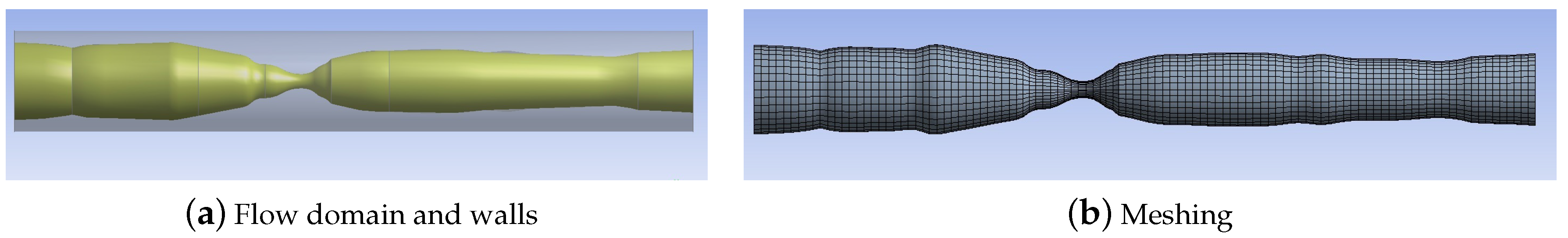
2.1. Flow Domain and Artery Wall

The variation of artery diameter along a stenosed section of the left coronary artery recorded in a patient angiogram is obtained. This information is used to recreate the flow geometry as shown in Figure 1a using ANSYS WORKBENCH: see [13] for details. The length of the artery section is 20.23 mm, and peak stenosis, which corresponds to 82% blockage of lumen diameter, is located at a distance of 8.3 mm from the inlet. The outer diameter of the artery at the inlet is set at 3.017 mm, and the wall thickness is 0.35 mm (i.e. lumen diameter at inlet is 2.317 mm). While recreating the geometry, it is assumed that the outer diameter of the artery (at the adventitial layer) remains constant at 3.017 mm, and that plaque formation is restricted to the intimal layer. Further, it is assumed in this study that the artery wall (including the plaque) can be modeled as a single material. The geometry is imported into ANSYS FLUENT for flow simulation.

2.2. Meshing and Grid Independence

The mesh in the flow domain is generated using elements of default shape set to a minimum size of 2 $\times {10}^{-4}$ m, and the number of elements is 19,928. The mesh in the domain occupied by the solid is generated using elements of default shape set to a minimum size of 2 $\times {10}^{-4}$ m, and the number of elements is 12,932. In both cases, the size of the element is determined by a grid independence study undertaken for the flow simulation, and for the wall deformation calculation: we required that results for the given element size not be more than 1% different from those in the smaller size. The meshed domain is shown in Figure 1b. A total of 3498 surface elements are used to impose pressure loading onto the internal walls of the artery.

2.3. Flow Modeling

We simulated the flow of blood using the (Non-Newtonian) Power-law model in ANSYS FLUENT. This model is given by:

$$\begin{array}{ccc}\hfill \mathbf{T}& =& -p\mathbf{1}+\mu \left(\dot{\gamma }\right)[\nabla \mathbf{v}+{\left(\nabla \mathbf{v}\right)}^T]\hfill \end{array}$$

(1)

$$\begin{array}{ccc}\hfill \mu \left(\dot{\gamma }\right)& =& m{\left(\dot{\gamma }\right)}^{(n-1)},\hfill \end{array}$$

(2)

where, $\mu$ is the dynamic viscosity of the model, and $\dot{\gamma }$ is the shear rate given by

$$\dot{\gamma }={\left[\frac{1}{2}tr{[\nabla \mathbf{v}+{\left(\nabla \mathbf{v}\right)}^T]}^2\right]}^{\frac{1}{2}}.$$

(3)

The Power-law model parameters m = 0.42 Pa$·s^n$, n = 0.61 are those for blood given in [14]. The Power-law model is preferred over other Non-Newtonian fluid models in ANSYS FLUENT (like the Carreau model) because it’s predictions for spatial variation of blood flow velocity along artery length are more gradual, and more in keeping with intuition (see [13] for details).

We assume volumetric flow rate at the inlet as 250 mL/min: this is the physiologic flow rate in the coronary artery as reported in [15]. Using the inlet diameter of 2.317 mm, the mean inlet velocity (which is specified as a boundary condition) in steady flow simulations is given as 0.988 m/s. For pulsatile flow simulation, we set the mean flow at 250 mL/min and add an oscillatory component of amplitude 156 mL/min [7] and frequency of 1.25 Hz (T = 0.8 s), so that the inlet velocity profile is specified as:

$${\overline{V}}_{inlet}=2\times 0.988\left[1+0.624\times sin(7.854·t)\right]m/s.$$

(4)

A user-defined function (UDF) is coded for this pulsatile flow inlet velocity, and imposed during simulations.

No-slip boundary condition is imposed for the velocity at the inner wall of the artery lumen.

We use the pressure-based solver, SIMPLE algorithm, available in ANSYS FLUENT to obtain the solution for the flow. Convergence criterion was set at ${10}^{-3}$ (absolute) for pressure and velocity components.

2.4. Fluid-Structure Interaction

The pressure field obtained in ANSYS FLUENT during blood flow is imported into the ANSYS STRUCTURAL package using the the ANSYS WORKBENCH toolbox. The inner walls of the artery are subject to the pressure field engendered during the flow, whereas the outer wall of the artery is traction-free. The two ends of the artery are held fixed during the FSI calculation. The resultant wall deformation is calculated using ANSYS STRUCTURAL.

2.5. Structural Modeling

The deformation of the artery wall when subject to the pressure generated during flow is calculated using ANSYS STRUCTURAL package.

The Rigid model is implemented for the artery wall by setting the ’Stiffness behavior’ to ’Rigid’ in the Solid Geometry table. The volumetric stress component in all the elastic material models is made negligible by prescribing a very small value ($2.7\times {10}^{-7}$) for the incompressibility parameter in the material properties.

The material properties for Rigid, Linear-Elastic (from [7]), Neo-Hookean, and Mooney-Rivlin materials in the steady flow simulation are as per

Table 1. Properties of wall material used in steady flow simulation.

Model	Parameter (s)	Value (s)
Rigid	$\mu$	∞
Linear-Elastic	$\mu$, $\nu$	10.346 kPa, 0.45
Neo-Hookean	$\mu$	10.346 kPa
Mooney-Rivlin	${\mu }_1,{\mu }_2$	10.346 kPa, 3.0 kPa

:

While the Neo-Hookean and Mooney Rivlin models are capable of capturing the large deformation non-linear elastic response of the artery, they do not incorporate the histological details of the artery wall: the walls of human artery are known to consist of two distinct symmetrical bands of collagen fibers that are helically wound around the artery axis [16,17]. This arrangement, combined with the soft-tissue nature of collagen and the intervening non-collagenous matrix, results in an anisotropic non-linear response of arteries when subject to loading. The Holzapfel model in [12] is the most accurate non-linear elastic model which incorporates two layers of fibers that lead to an anisotropic response under loading.

2.6. Implementation of the Holzapfel Model

The two-layer non-linear anistropic elastic model in [12] is given as a schematic in [12]. This model requires a UMAT which is more advanced than that for a single-layer model: the single-layer anisotropic non-linear elastic model is selected for the implementation, and not the double-layer model. The schematic of the single-layer model is given in Figure 2.

This model is not available among the suite of models in ANSYS. Hence, it has to be coded using a user material function (UMAT). ANSYS requires that the Jaumann derviative ($\stackrel{\nabla }{\underline{\mathbf{D}}}$) of the tangent stiffness matrix ($\underline{\mathbf{D}}$) be coded in a Voigt-type notation that is used for all matrices in ANSYS. We detail the derivation below for these matrices.

The strain energy function defined in [12] is given by:

$$\varphi ={\varphi }_{iso}\left(I_1\right)+{\varphi }_{aniso}(I_4,I_6),$$

(5)

where $I_1$ is the first invariant of the Right Cauchy-Green stretch tensor $\mathbf{C}$ (= ${\mathbf{F}}^T\mathbf{F}$), and $I_4,I_6$ are the fourth, and sixth invariants calculated in Equations (6)–(9) below. Here ${\mathbf{a}}_{01}$, and ${\mathbf{a}}_{02}$ are the vectors denoting fiber orientation of collagen in the artery wall (separated by angle $\beta$: see Figure 2).

$$\begin{array}{ccc}\hfill {\mathbf{A}}_{\mathbf{1}}& =& {\mathbf{a}}_{01}\otimes {\mathbf{a}}_{01},\hfill \end{array}$$

(6)

$$\begin{array}{ccc}\hfill {\mathbf{A}}_{\mathbf{2}}& =& {\mathbf{a}}_{02}\otimes {\mathbf{a}}_{02},\hfill \end{array}$$

(7)

$$\begin{array}{ccc}\hfill I_4& =& \mathbf{C}:{\mathbf{A}}_{\mathbf{1}},\hfill \end{array}$$

(8)

$$\begin{array}{ccc}\hfill I_6& =& \mathbf{C}:{\mathbf{A}}_{\mathbf{2}},\hfill \end{array}$$

(9)

We define the isochoric part of the stretch tensor as:

$$\overline{\mathbf{C}}=J_C^{\frac{1}{3}}\mathbf{C}.$$

(10)

We then redefine the strain energy function as below:

$$\varphi ={\varphi }_{iso}\left({\overline{I}}_1\right)+{\varphi }_{aniso}({\overline{I}}_4,{\overline{I}}_6),$$

(11)

where the invariants are defined in like manner as Equations (6)–(9), but using $\overline{\mathbf{C}}$.

The individual components of the (isochoric) strain energy are given as follows [12]:

$$\begin{array}{ccc}\hfill {\varphi }_{iso}\left({\overline{I}}_1\right)& =& \frac{c}{2}\left({\overline{I}}_1-3\right),\hfill \end{array}$$

(12)

$$\begin{array}{ccc}\hfill {\varphi }_{aniso}({\overline{I}}_4,{\overline{I}}_6)& =& \frac{k_1}{2k_2}\sum _{i=4,6}\left[e^{\left(k_2{({\overline{I}}_i-1)}^2\right))}-1\right].\hfill \end{array}$$

(13)

The Cauchy stress is given by:

$$\mathbf{T}=\frac{1}{J}\frac{\partial \varphi \left(F\right)}{\partial \mathbf{F}}{\mathbf{F}}^T,$$

(14)

ANSYS requires that the tangent stiffness matrix be calculated in terms of the second Piola-Kirchchoff stress (Equation (15)), and with respect to the Lagrangian strain tensor given in Equation (16):

$$\overline{\mathbf{S}}=2\frac{\partial \varphi }{\partial \mathbf{C}},$$

(15)

$$\mathbf{E}=\frac{1}{2}\left(\mathbf{C}-\mathbf{I}\right).$$

(16)

Hence, evaluation of $\overline{\mathbf{S}}$ is given below:

$$\overline{\mathbf{S}}=2\frac{\partial \varphi ({\overline{I}}_1,{\overline{I}}_4,{\overline{I}}_6)}{\partial \overline{\mathbf{C}}}\frac{\partial \overline{\mathbf{C}}}{\partial \mathbf{C}}.$$

(17)

The first term is evaluated using standard tensor calculus, and simplifies as:

$$\frac{\partial \varphi }{\partial \overline{\mathbf{C}}}=\frac{c}{2}\mathbf{I}+k_1({\overline{I}}_4-1)e^{\left(k_2{({\overline{I}}_4-1)}^2\right)}{\mathbf{A}}_{\mathbf{1}}+k_1({\overline{I}}_6-1)e^{\left(k_2{({\overline{I}}_6-1)}^2\right)}{\mathbf{A}}_{\mathbf{2}}$$

(18)

The second term is simplified as follows:

$$\begin{array}{cc}\hfill \frac{\partial \overline{\mathbf{C}}}{\partial \mathbf{C}}& =\left(-\frac{J_C^{-4/3}}{3}\frac{\partial J_C}{\partial \mathbf{C}}\mathbf{C}\right)+\left(J_C^{-1/3}\mathbf{I}\right),\hfill \\ & =\left(-\frac{J_C^{-4/3}}{3}{J}_C{\mathbf{C}}^{-1}\mathbf{C}\right)+\left(J_C^{-1/3}\mathbf{I}\right),\hfill \\ & =\left(-\frac{J_C^{-1/3}}{3}\mathbf{I}\right)+\left(J_C^{-1/3}\mathbf{I}\right),\hfill \\ & =\frac{2}{3}{J}_C^{-1/3}\mathbf{I}.\hfill \end{array}$$

(19)

Hence, $\overline{\mathbf{S}}$ reduces to:

$$\overline{\mathbf{S}}=\frac{4}{3}{J}_C^{-1/3}\frac{\partial \varphi }{\partial \overline{\mathbf{C}}}.$$

(20)

The tangent stiffness matrix $\mathbf{D}$ is given by:

$$\begin{array}{cc}\hfill \mathbf{D}& =\frac{\partial \overline{\mathbf{S}}}{\partial \mathbf{E}}\hfill \\ & =\frac{\partial \overline{\mathbf{S}}}{\partial \overline{\mathbf{C}}}\frac{\partial \overline{\mathbf{C}}}{\partial \mathbf{E}}\hfill \\ & =\frac{\partial \overline{\mathbf{S}}}{\partial \overline{\mathbf{C}}}\left(\frac{4}{3}{J}_C^{-2/3}\mathbf{I}\right)\hfill \end{array}$$

(21)

Again, the first term is evaluated as follows:

$$\begin{array}{cc}\hfill \frac{\partial \overline{\mathbf{S}}}{\partial \overline{\mathbf{C}}}& =[-\frac{c}{3}{\mathbf{C}}^{-1}]+[-\frac{2}{3}{k}_1({\overline{I}}_4-1)e^{\left(k_2{({\overline{I}}_4-1)}^2\right)}{\mathbf{C}}^{-1}{\mathbf{A}}_{\mathbf{1}}]\hfill \\ & =+[-\frac{2}{3}{k}_1({\overline{I}}_6-1)e^{\left(k_2{({\overline{I}}_6-1)}^2\right)}{\mathbf{C}}^{-1}{\mathbf{A}}_{\mathbf{2}}]\hfill \\ & =+[-\frac{4}{3}{J}^{-2/3}{k}_1{e}^{\left(k_2{({\overline{I}}_4-1)}^2\right)}{\mathbf{A}}_{\mathbf{1}}^2]+[-\frac{8}{3}{J}^{-2/3}{k}_1{k}_2{e}^{\left(k_2{({\overline{I}}_4-1)}^2\right)}{\mathbf{A}}_{\mathbf{1}}^2]\hfill \\ & =+[-\frac{4}{3}{J}^{-2/3}{k}_1{e}^{\left(k_2{({\overline{I}}_6-1)}^2\right)}{\mathbf{A}}_{\mathbf{2}}^2]+[-\frac{8}{3}{J}^{-2/3}{k}_1{k}_2{e}^{\left(k_2{({\overline{I}}_6-1)}^2\right)}{\mathbf{A}}_{\mathbf{2}}^2]\hfill \end{array}$$

The user material (UMAT) function is written for ANSYS STRUCTURAL using ANSYS specified syntax to implement this model with the following constants: c = 10.346 kPa, $k_1$ = 2.3632 kPa, $k_2$ = 0.8393 kPa [12].

We obtain the syntax for Neo-Hookean model from [18]; further we confirmed that our UMAT code is correct by comparing with the formulation in [19] for the same Holzapfel (MA) model.

3. Results

3.1. Steady State Flow

The contours of velocity (for the inner fluid) and pressure (at the wall) obtained for steady flow in the stenosed geometry are shown in Figure 3, respectively.

3.2. Wall Deformation in Steady Flow

The results of wall deformation for the four models are given in Figure 4. Naturally, the Rigid wall model shows zero deformation. The Linear-elastic model predicts the maximum deformation, whereas the Neo-Hookean model and Mooney-Rivlin model show progressively less values. The Neo-Hookean model predicts values that are quite close to those predicted by the Linear Elastic model.

The constitutively accurate Holzapfel model is implemented, and the contours of wall deformation along the artery length for both Neo-Hookean model and Holzapfel model are plotted in Figure 5.

Further, the predictions of wall deformation along the length of the artery section, for both the Holzapfel and Neo-Hookean models, is plotted in Figure 6. It is seen that, in steady flow, the Holzapfel model predicts maximum deformation that is only around 50% that predicted by the Neo-Hookean model. This has important consequences in the planning of angioplasty.

3.3. Wall Deformation in Pulsatile Flow

We then obtain the variation of deformation at location of maximum stenosis during pulsatile flow for the physiologically accurate Holzapfel model, and the results are given in Figure 7. These results are consistent with those obtained in steady flow.

4. Discussion

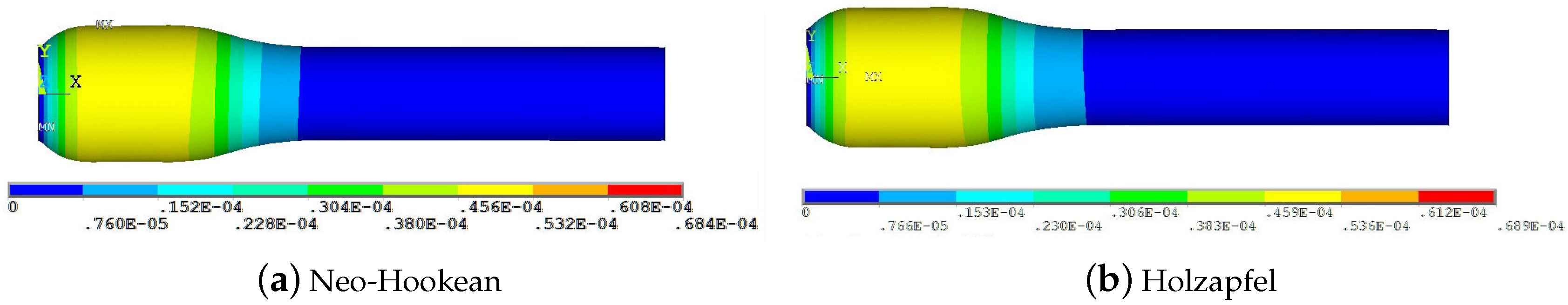
We documented the effect of varying wall flexibility on the deformation of the artery wall in a patient-derived geometry of a stenosed left coronary artery.

In steady flow,

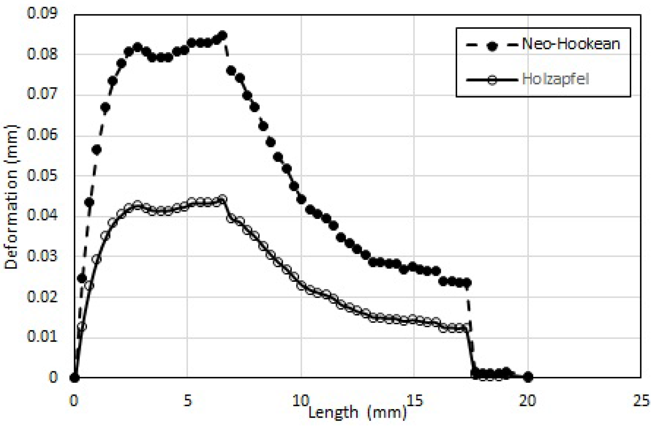
• Maximum wall deformation predicted by the physiologically accurate Holzapfel model is ≈50% that predicted by the Neo-Hookean model.
• Maximum wall deformation predicted is highest for the Linear-Elastic model.
• Wall deformation of both Neo-Hookean and Mooney-Rivlin model are consistently lower (5.6% and 66.7%, respectively) than that of the Linear-Elastic model (for the same shear modulus).
• Maximum wall deformation occurs well before the peak stenosis location: 6mm from the entrance, compared to 8.3 mm where the peak stenosis is located.

Further, the results for wall deformation of Holzapfel model during pulsatile flow are consistent with those obtained in steady flow.

This computational study is intended to get us closer to the use of locally available computational simulations to assist revascularization procedures, and thereby bring down the cost of such procedures. The calculations of Pulsatile and Steady flow-induced wall deformation in patient-derived stenosed coronary artery with physiologically accurate model are first of its kind. These results help immensely in the planning of angioplasty: for instance, the fact that the wall deformation for Holzapfel model is only ≈50% that of the Neo-Hookean model means that the estimate of pressure required within the angioplasty balloon needs to be recalibrated to successfully produce the same deformation. This study (taken in combination with that in [13]) outlines a simple procedure to recreate the geometry of a stenosed artery, simulate the flow within, and use FSI to calculate the maximum (and minimum) deformation of the artery wall. The deformation of the artery wall, which is severely underestimated by assuming the wall is rigid, needs to be accounted for when calculating the pressure to be applied to the angioplasty balloon. Not doing so can only lead to compromise on the effectiveness of the procedure.

Novel though it may be, there are some aspects of the study that need extension before the procedure can be widely advocated. One limitation is that the FSI is only one-way, and not two-way: i.e. the procedure does not recalculate the pressure field in the deformed configuration, and iterate for the wall deformation. The second limitation is that the entire artery wall including the plaque is modeled as a single material whereas the reality is not that: the plaque (which consists of lipids surrounding a necrotic core) is an entirely different material from the artery wall with possibly different material parameters. Hence the plaque is better modeled as an isotropic material with material parameters that are possibly much smaller than those of the artery. Such limitations must be addressed in a future study to obtain wall deformation that is much closer to reality.