Article

Horizontal Cellular Oscillations Caused by Time-Periodic Resonant Thermal Forcing in Weakly Nonlinear Darcy-Bénard Convection

by
Ibrahim M. Jais
1 and
D. Andrew S. Rees
2,*
1
Department of Mathematical Sciences, Universiti Teknologi Malaysia, 81300 Skudai, Malaysia
2
Department of Mechanical Engineering, University of Bath, Bath BA2 7AY, UK
*
Author to whom correspondence should be addressed.
Fluids 2017, 2(4), 60; https://doi.org/10.3390/fluids2040060
Submission received: 14 September 2017 / Revised: 25 October 2017 / Accepted: 27 October 2017 / Published: 4 November 2017
(This article belongs to the Special Issue Convective Instability in Porous Media)

Abstract

:
The onset of Rayleigh-Bénard convection in a horizontally unbounded saturated porous medium is considered. Particular attention is given to the stability of weakly nonlinear convection between two plane horizontal surfaces heated from below. The primary aim is to study the effects on postcritical convection of having small amplitude time-periodic resonant thermal forcing. Amplitude equations are derived using a weakly nonlinear theory and they are solved in order to understand how the flow evolves with changes in the Darcy-Rayleigh number and the forcing frequency. When convection is stationary in space, it is found to consist of one of two different types depending on its location in parameter space: either a convection pattern where each cell rotates in the same way for all time with a periodic variation in amplitude (Type I) or a pattern where each cell changes direction twice within each forcing period (Type II). Asymptotic analyses are also performed (i) to understand the transition between convection of types I and II; (ii) for large oscillation frequencies and (iii) for small oscillation frequencies. In a large part of parameter space the preferred pattern of convection when the layer is unbounded horizontally is then shown to be one where the cells oscillate horizontally—this is a novel form of pattern selection for Darcy-Bénard convection.

1. Introduction

The classical Bénard problem as applied to a porous medium was first studied by Horton and Rogers (1945) [1] and independently by Lapwood (1948) [
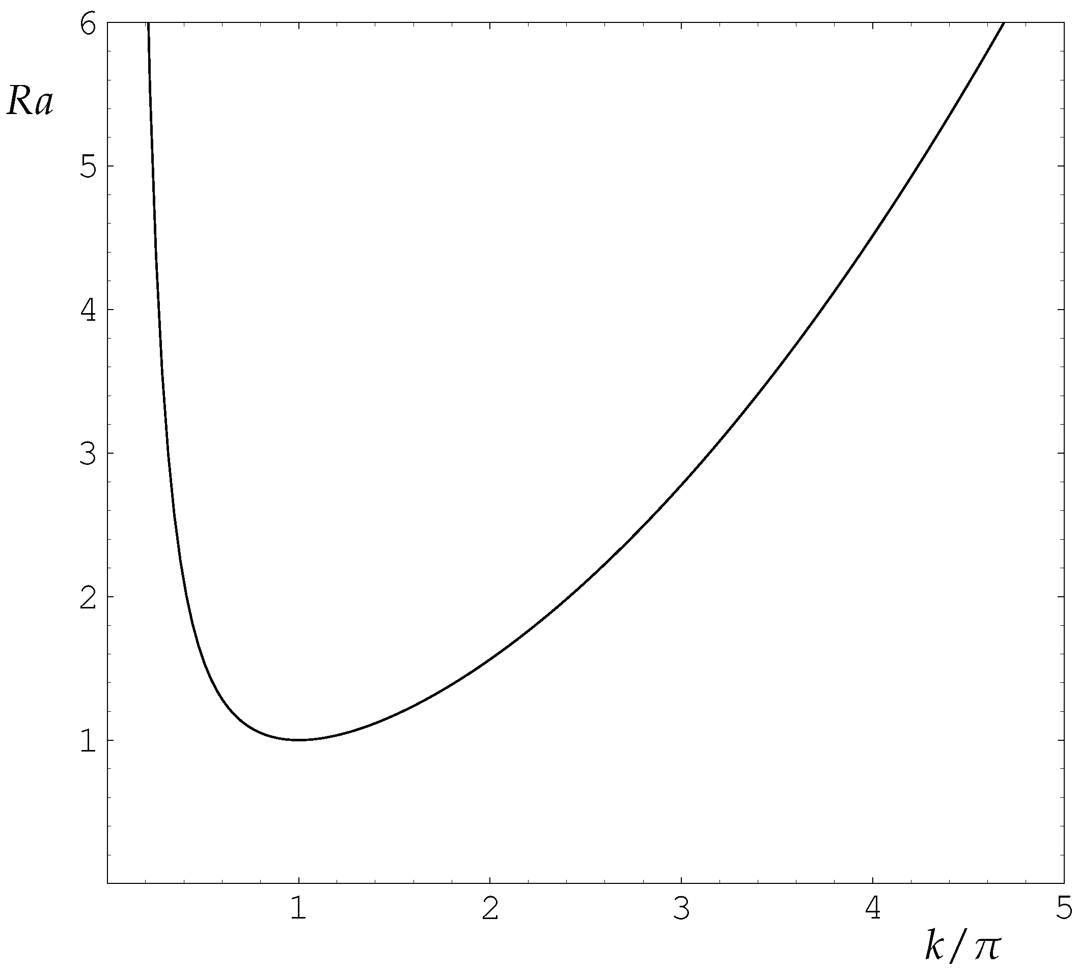
2]; these authors considered the onset of convection in a horizontal saturated porous layer heated uniformly from below. Using a linear stability theory, the neutral curve which relates the Darcy-Rayleigh number, R a , to the wavenumber, k, may be shown to take the form,
R a = ( k 2 + n 2 π 2 ) 2 k 2 ,
(see Rees 2000, for example) [3] where the value of n corresponds to the number of rolls which are stacked above one another in the layer. This variation of R a with k is shown in Figure 1 and it may be shown easily that the minimum/critical value is R a c = 4 π 2 , which occurs when k = π and n = 1 . These values correspond to rolls with a square cross-section.
Palm et al. (1972) [4] subsequently analysed the moderately supercritical flow using a series representation in terms of powers of ( R a R a c ) / R a . A very detailed numerical stability analysis was undertaken by Straus (1974) [5] who delineated the region in ( R a , k ) -space within which steady rolls form the stable planform of convection.
The general topic of Darcy-Bénard convection continues to grow rapidly as further effects, realism and/or practical application are added to the original Horton-Rogers-Lapwood configuration [2,6]. Reviews have been presented by Rees (2000) [3] and Tyvand (2002) [7], but the topic has continued to be the subject of substantial interest in the time since then, and therefore we would refer the reader to the latest edition of Nield and Bejan (2017) [8] for an up-to-date account of the topic.
In the present paper, we shall confine our interest to the role played by boundary imperfections, itself a well-researched subtopic. It is widely recognised that completely uniform and idealised boundary conditions are not easily achieveable in practice, and therefore authors such as Riahi (1983) [9], Saleh et al. (2011) [10], Motjabi and Rees (2011) [1] and Rees and Mojtabi (2011) [11] have concerned themselves with more realistic boundary conditions where the perfectly conducting bounding surfaces are replaced by conducting solids. The resulting stability properties are influenced profoundly by the nature of the solids used and their thickness. Thus it is possible for perfectly conducting boundary conditions on the outer surfaces to give rise to stability properties which are more closely associated with constant heat flux surfaces, and vice versa. It is also possible for roll solutions to be unstable in some circumstances, in which case convection with a square planform forms the preferred pattern (see Riahi 1993, Rees and Mojtabi 2011) [11].
In a series of papers, Rees and Riley (1986, 1989a, 1989b) [12,13,14] and Rees (1990) [15] considered the effect of small-amplitude boundary variations on both the onset of convection and convection within the weakly nonlinear regime. Depending on the wavenumber of the variation, the preferred pattern of convection may take the form of rolls, wavy rolls, rectangular cells or exhibit other unusual properties. Other papers of this type include those by Vozovoi and Nepomnyaschii (1974) [16], Tavantzis et al. (1978) [17], O’Sullivan and McKibbin (1986) [18] and Riahi (1993, 1995) [9,19,20].
A little later, Mamou et al. (1996) [21] and Banu and Rees (2001) [22] applied thermal boundary variations of the form cos π ( x U t ) , which correspond to travelling thermal waves at the critical spatial wavenumber, π . The former paper considered strongly supercritical convection using fully numerical methods, while the latter applied a weakly nonlinear theory in order to understand the subtle details which arise closer to the onset of convection. The effect of having a forcing wave speed, U, is to cause a competition between the tendency of the rolls to remain stationary, which is what happens naturally in a layer without such imperfections, and the tendency to follow the forcing wave. It was found that there is a catastrophic transition between the wave-following regime and the quasi-stationary regime in that the amplitude and horizontal velocity of the convection pattern change suddenly as the Darcy-Rayleigh number increases. This system was also found to display hysteresis, for the reverse transition which occurs as the Rayleigh number decreases, does so at a different value of the Rayleigh number.
The present paper is concerned with a physical configuration for which convection cells also have a tendency to move. For the Darcy-Bénard problem one of the easiest ways in which this may arise is when the fluid is also subject to a horizontal pressure gradient. Prats (1967) [23] showed that the convection cells then move with precisely the same velocity as the pressure-gradient-induced flow which exists in the absence of heating. Thus the dynamics of the ensuing convection are precisely the same as that for a layer without the background flow when it is considered in a frame of reference which is moving with the background flow. An interesting variation on this Darcy-Bénard-Prats problem was studied by Dufour and Néel (1996) [24] where a uniform horizontal flow is injected into a horizontally semi-infinite porous layer heated from below. In general the flow remains roughly uniform near to injection and there exists a spatial transition towards the time-periodic flow described by Prats (1967) [23]. The length of the transition region depends on the magnitudes of the injection velocity, Q (a Péclet number) and the Darcy-Rayleigh number, increasing as Péclet number increases but decreasing as the Darcy-Rayleigh number increases; these phenomena are related to the phase diffusion speed of the convection cells. A much more recent paper by Rees and Mojtabi (2013) [1] shows that the presence of solid conducting boundaries serves to reduce the phase speed of the convecting cells. This reduction may be attributed to what might be called a thermal drag which arises due to the fact that the time-varying convection mode has to move through a stationary boundary of finite height.
Another mechanism which relies neither on an external pressure gradient nor on moving boundary conditions to induce phase drift is when convection takes place in a cylindrical container with a circular planform. Although no studies have yet been published on such flows in porous media, it is well-known that such a variant of the classical Bénard problem may sometimes exhibit a rotating spiral convection pattern even though all the boundary conditions are steady and uniform; see Plapp et al. (1998) [25].
In this paper we consider thermal forcing of the form cos ω t cos π x , and this may be regarded as the standing wave counterpart to the work of Banu and Rees (2001) [22]. Although this thermal forcing is now stationary in space, we shall show later that it remains possible for rolls to exhibit a time-periodic horizontal motion. As shall be seen, the reason for this periodic motion is that the preferred phase of the convection cells depends (in a quasi-static sense) on the sign of the forcing amplitude, cos ω t , and therefore the phase of the cells is drawn towards two different fixed points during the two different parts of the forcing cycle. Our subsequent analyses involve a derivation of the weakly non-linear amplitude equations, together with both numerical simulations and asymptotic analyses of those amplitude equations. Attention is also focused on the transition between two different types of stationary motion, and on a twitching motion at high Rayleigh numbers where cells execute small-amplitude periodic movements in phase.

2. Governing Equations

Darcy’s law gives the most basic equation governing fluid flows in a porous medium. It is the macroscopic law which relates the fluid flux to the applied pressure gradient. For buoyancy-affected flows of a Boussinesq fluid, where the porous medium is assumed to be homogeneous, nondeformable and isotropic, the dimensional equations which govern the fluid motion are,
u ¯ = K μ p ¯ x ¯ , v ¯ = K μ p ¯ y ¯ , w ¯ = K μ p ¯ z ¯ + ρ f g β K μ T T c .
In these equations all the terms take their common meanings. The coordinates x ¯ and y ¯ are in the horizontal directions, while z ¯ is vertically upwards. T is the temperature of the saturated medium, T c is the mean upper (cold) boundary temperature, p ¯ is the pressure, K the permeability, μ the viscosity, g gravity, ρ f a reference density of the fluid, and β the coefficient of cubical expansion of the fluid. The quantities u ¯ , v ¯ and w ¯ , correspond to the fluid seepage velocities in the x ¯ , y ¯ and z ¯ directions, respectively.
The full equations are completed by the equation of continuity,
u ¯ x ¯ + v ¯ y ¯ + w ¯ z ¯ = 0 ,
and the heat transport equation,
σ T t + u ¯ T x ¯ + v ¯ T y ¯ + w ¯ T z ¯ = κ 2 T x ¯ 2 + 2 T y ¯ 2 + 2 T z ¯ 2 ,
where κ is the thermal diffusivity of the saturated porous medium and,
σ = ( 1 ϕ ) ( ρ c ) s + ϕ ( ρ c ) f ( ρ c ) f ,
is the heat capacity ratio of the saturated medium to that of the fluid. The value, c, is the specific heat and ρ the density of the medium, with the subscripts f and s referring to the fluid and solid phases, respectively.
The nondimensionalisation of Equations (2)–(4) is achieved using the following substitutions,
( x , y , z ) = ( x ¯ , y ¯ , z ¯ ) d , ( u , v , w ) = d κ ( u ¯ , v ¯ , w ¯ ) ,
p = K κ μ p ¯ , θ = T T c T h T c , t = κ d 2 σ t ¯ ,
where d is the height of the layer. Here, T c and T h are the cold (upper) and hot (lower) mean temperatures of the horizontal bounding surfaces. Hence, the non-dimensional equations are,
u x + v y + w z = 0 ,
( u , v , w ) = p x , p y , p z + ( 0 , 0 , R a θ ) ,
θ t + u θ x + v θ y + w θ z = 2 θ x 2 + 2 θ y 2 + 2 θ z 2 .
In the above, the parameter,
R a = ρ f g β ( T h T c ) K d μ κ ,
is the Darcy-Rayleigh number; the usual clear-fluid Rayleigh number may be obtained by replacing the permeability, K, by d 2 . The Darcy-Rayleigh number expresses the balance between buoyancy and viscous forces.
Assuming that the flow is two dimensional, then v = 0 and all the derivatives with respect to y may be neglected. Hence, by introducing the stream function, ψ , using u = ψ z and w = ψ x , not only is Equation (8) satisfied but Equations (9) and (10) become,
2 ψ x 2 + 2 ψ z 2 = R a θ x ,
θ t + ψ x θ z θ x ψ z = 2 θ x 2 + 2 θ z 2 .
Both of the equations above are to be solved analytically using a weakly nonlinear analysis.
The boundary surfaces are considered to be impermeable. The thermal boundary conditions comprise a combination of heating from below and a small-amplitude variation which is periodic in both time and space. Therefore the boundary conditions are
z = 0 : ψ = 0 , θ = 1 + δ cos ω ^ t cos π x , z = 1 : ψ = 0 , θ = δ cos ω ^ t cos π x ,
where δ 1 is the amplitude of the thermal forcing and ω ^ is its nondimensional temporal frequency.

3. Weakly Nonlinear Analysis

In this section we shall carry out a weakly nonlinear analysis in order to obtain a complex Landau equation for the amplitude of convection in the presence of the thermal boundary imperfections given in Equation (14). This will be undertaken using the scalings which were used in Rees and Riley (1989a) [13] and Banu and Rees (2002) [22], and which are suitable for those cases where the wavenumber of the imperfection takes the critical value. We follow the methodology introduced by Newell and Whitehead (1969) [26] for the Bénard problem.
Therefore we shall set the amplitude of convection to be of O ( ϵ ) and the Darcy-Rayleigh number shall be within a distance of O ( ϵ 2 ) of its critical value, 4 π 2 . Given that the imperfection has the critical wavenumber, we need to set δ = ϵ 3 1 ; see Rees and Riley (1986,1989a) [12,13]. The appropriate time scale is of O ( ϵ 2 ) . Equations (12) and (13) may now be expanded using the following asymptotic series,
ψ = ϵ ψ 1 + ϵ 2 ψ 2 + ϵ 3 ψ 3 + ,
θ = 1 z + ϵ θ 1 + ϵ 2 θ 2 + ϵ 3 θ 3 + cos 2 ω ˜ τ cos π x + ,
and, given the above observations, we set
R a = R 0 + ϵ 2 R 2 + , ω ˜ = ϵ 2 ω ^ , τ = 1 2 ϵ 2 t ,
where R 0 = 4 π 2 . The leading term in Equation (16) is the linear conduction profile while the additional cosine term at O ( ϵ 3 ) renders the thermal boundary conditions for θ 3 to be homogeneous (see Equation (14)).
At O ( ϵ ) , the leading order disturbance equations are,
ψ 1 x x + ψ 1 z z R 0 θ 1 x = 0 ,
θ 1 x x + θ 1 z z + ψ 1 x = 0 .
These homogeneous equations form the linearised stability problem for the uniformly heated layer, and are to be solved subject to the following homogeneous Dirichlet boundary conditions,
ψ 1 = θ 1 = 0 on both z = 0 and z = 1 ;
identical conditions will also apply for ψ i and θ i , i = 2 , 3 . We choose to use the following roll eigensolutions,
ψ 1 = i π A e i π x A ¯ e i π x sin π z , θ 1 = 1 2 A e i π x + A ¯ e i π x sin π z ,
where A = A ( τ ) is a complex amplitude which is a function of the slow timescale, τ . The complex forms used in Equation (21) allow for a straightforward modelling of phase variations in the solutions.
At O ( ϵ 2 ) the equations for ψ 2 and θ 2 are,
ψ 2 x x + ψ 2 z z R 0 θ 2 x = 0 ,
θ 2 x x + θ 2 z z + ψ 2 x = ψ 1 x θ 1 z ψ 1 z θ 1 x .
When the solutions given in Equations (21) are substituted into Equation (23) the latter becomes,
θ 2 x x + θ 2 z z + ψ 2 x = π 3 A A ¯ sin 2 π z ,
and therefore ψ 2 and θ 2 are found to be,
ψ 2 = 0 , θ 2 = 1 4 π A A ¯ sin 2 π z .
At O ( ϵ 3 ) the equations for ψ 3 and θ 3 are,
ψ 3 x x + ψ 3 z z R 0 θ 3 x = R 2 θ 1 x R 0 π cos 2 ω ˜ τ sin π x ,
θ 3 x x + θ 3 z z + ψ 3 x = ψ 1 x θ 2 z ψ 1 z θ 2 x + ψ 2 x θ 1 z ψ 2 z θ 1 x + 1 2 θ 1 τ + π 2 cos 2 ω ˜ τ sin π x .
After the substitution of Equations (21) and (25), the above equations become,
ψ 3 x x + ψ 3 z z R 0 θ 3 x = 1 2 i π R 2 A e i π x A ¯ e i π x sin π z + 4 π 3 cos 2 ω ˜ τ sin π x ,
θ 3 x x + θ 3 z z + ψ 3 x = 1 2 i π 4 A A ¯ A e i π x + A ¯ e i π x sin 3 π z sin π z 1 4 A τ e i π x + A ¯ τ e i π x sin π z + π 2 cos 2 ω ˜ τ cos π x .
The inhomogeneous terms in Equations (28) and (29) contain components which are proportional to the eigensolution of the homogeneous form of the equations, namely, the solutions given in Equation (21). The value for R 2 is presently arbitrary but in general this system of equations cannot be solved unless R 2 takes a specific value. The derivation of a solvability condition will yield the desired amplitude equation for A in terms of R 2 , the satisfaction of which guarantees the solution of Equations (28) and (29) up to an arbitrary multiple of the eigensolution.
If Equations (28) and (29) are written in the form,
ψ 3 x x + ψ 3 z z R 0 θ 3 x = R 1 , θ 3 x x + θ 3 z z + ψ 3 x = R 2 ,
and if we define the quantities, ψ = i π e i π x sin π z and θ = 1 2 e i π x sin π z , which are the coefficients of A ¯ in Equation (21), then the following identity may be formed:
0 1 0 2 ψ 3 x x + ψ 3 z z R 0 θ 3 x ψ + R 0 θ 3 x x + θ 3 z z + ψ 3 x θ d x d z = 0 1 0 2 R 1 ψ + R 0 R 2 θ d x d z .
The left hand side of Equation (31) may be shown to be precisely equal to zero by using integration by parts, and thus the solvability condition is that,
0 1 0 2 R 1 ψ + R 0 R 2 θ d x d z = 0 .
Upon application of this solvability condition to Equations (28) and (29) we obtain the following amplitude (i.e., Landau) equation,
A τ = R 2 A π 4 A 2 A ¯ + 8 π cos 2 ω ˜ τ .
The coefficients of the last two terms of Equation (33) may be simplified by rescaling A, τ and R 2 in order to obtain the following canonical form of the amplitude equation,
A τ = R 2 A A 2 A ¯ + cos ω τ .
The scalings which are required to do this are,
ω = ω ˜ 2 π 2 , A = 1 2 π A , R 2 = R 2 4 π 2 , τ = 4 π 2 τ .
If we omit the asterisks for simplicity of presentation, then the complex amplitude equation governing weakly nonlinear convection is,
A t = R 2 A A 2 A ¯ + cos ω t ,
where τ has been replaced by t for simplicity of presentation from this point onwards, and this t should not be confused with that used in §§1 and 2. The rest of the paper is devoted to the properties of the real and complex solutions of this equation. For any given ω the forcing period is T = 2 π / ω .

4. Real Solutions of the Amplitude Equations

4.1. Initial Considerations and Context

Rees and Riley (1986) [12] obtained the following amplitude equation for a steady perfectly resonant imperfection,
A t = R 2 A A 2 A ¯ + 1 .
and this is equivalent to the setting of ω = 0 in the present paper. The steady solutions of Equation (37) are shown in Figure 2 and this Figure shows that no zero-amplitude solution is possible. When R 2 < 0 a unique solution is obtained, and it satisfies the asymptotic relation, A R 2 1 , when R 2 has a large amplitude. But as R 2 increases, the amplitude of this solution branch also increases until it approaches asymptotically to A R 2 1 / 2 when R 2 is large and positive. The upper branch of this bifurcation diagram is stable. However, when R 2 > 3 / 2 2 / 3 , there exist two other solution branches, and both of these are unstable with respect to perturbations in phase when the porous layer is unbounded horizontally. The middle branch is also unstable unconditionally to perturbations in amplitude.
An alternative way of visualizing the stability properties of Equation (37) which are described above is shown in Figure 3. In this Figure are displayed solution trajectories of A as a complex amplitude for different values of R 2 and for different initial conditions placed on a unit circle in the complex plane. For all choices of R 2 , the values of A converge onto the solution which is on the positive real axis. When R 2 is sufficiently large and the initial condition is close to the negative real axis, then the amplitude increases rapidly to close to R 2 1 / 2 and then the phase varies relatively slowly until the positive real axis is reached. The variation in phase is equivalent to a slow physical migration of the rolls towards the stable location, and this means that | A | has also been maximised.
The usefulness of the above picture lies in the fact that it gives a good insight into what might happen when ω is no longer zero. Thus when cos ω t > 0 , Figure 3 gives an indication of the trajectories, while the mirror image about the vertical axis corresponds to when cos ω t < 0 . Therefore we may draw an a priori conclusion that there might be the possibility of cases where there could be permanent oscillations in phase, given that a positive real value of A forms the attractive stable solution when cos ω t > 0 and its negative counterpart does so when cos ω t < 0 .

4.2. Numerical solutions

We may expand Equation (36) by splitting it into its real and imaginary components: A ( t ) = B ( t ) + i C ( t ) , where B ( t ) and C ( t ) are both real. This yields the following pair of coupled non-linear equations,
B t = R 2 B ( B 2 + C 2 ) B + cos ω t ,
and
C t = R 2 C ( B 2 + C 2 ) C .
From Equation (39) we see that C = 0 is a possible solution, which corresponds to real values of A and, given the definition of A in Equations (21), convection is exactly in phase with the thermal forcing when both A and cos ω t are of the same sign.
In this subsection we shall concentrate solely on real solutions of Equation (38) with C = 0 , namely,
B t = R 2 B B 3 + cos ω t .
This equation was solved using the classical 4 th order Runge Kutta method with at least 2000 timesteps within a period until all transients have decayed and a steady periodic state is achieved. Integration took place over a whole number of periods of the forcing, i.e., up to the time t m a x = N ( 2 π / ω ) where N is an integer. For each period, the solution was compared with that over the previous period, and when the maximum absolute difference over all the time steps was less than 10 6 then convergence was deemed to have occurred.
In Figure 4 steady real periodic solutions are shown for a variety of frequencies, ω , and for a range of values of R 2 lying between 5 and 3. These curves are typical of all periodic real solutions. There are two different types of solution which occur as R 2 and ω are varied:
(1)
a single-signed oscillation, which we call Type I,
(2)
solutions taking both positive and negative amplitudes, which we call Type II.
It is clear from Figure 4 that, for all values of ω , single-signed solutions (Type I) always exist when R 2 is sufficiently large and that double-signed solutions (Type II) exist when R 2 is negative. However, the transition between these two states isn’t straightforward to see in this Figure. When the forcing period is large (e.g., when T = 100 ) there appears to be a sudden transition between the two Types. However, when the forcing period is small (such as when T = 1 and T = 5 ) the solution curves simply descend as R 2 decreases. There will be a precise value of R 2 (which we will call R 2 zero ) at which the minimum value of B is zero; these values are listed in Table 1. But the consequence is that there appears to be an intermediate range of R 2 which seems to be transitional between the two Types.
Further analysis of these curves indicates that the characterisation of the two Types based on whether a particular curve is single-signed or double-signed is too simplistic. A much better alternative is to consider the variation in the maximum and minimum values of B over one period; such curves are displayed in Figure 5. Concentrating first on the continuous lines for T = 5 and for low values of R 2 , we see that B max + B min = 0 , and therefore the corresponding solution curves for B are double-signed and are of Type II. Once R 2 reaches roughly 0.838 there is a clear bifurcation to a new form of solution, and it is this which should be labelled as being of Type I. Again concentrating on the continuous curves, we see that B max and B min still have the opposite sign for a further small range of values of R 2 , but once R 2 exceeds roughly 1.043 the solution then becomes single-signed.
In Figure 5 the continuous curves correspond to the use of B ( t = 0 ) > 0 as the initial condition, whereas the dotted lines correspond to B ( t = 0 ) < 0 , or, equivalently, to solutions with a phase-shift of π compared with the solutions with the positive initial condition. Inclusion of these latter curves give rise to sets of curves which are more obviously of supercritical bifurcation type, and it is this point of bifurcation which marks the exact transition between solutions of the two Types. Although we shall not demonstrate it, Type II solutions also exist above the bifurcation point and have been computed, but they are unstable.
Given that the bifurcation point is where the Type II solutions become unstable, we may determine these points numerically. If we set A = B + D into Equation (40), where D is both real and asymptotically small, then we obtain the following linearised equation for D:
D t = ( R 2 3 B 2 ) D .
The bifurcation point now corresponds to nonzero solutions for D for which D ( 0 ) = D ( 2 π ω ) . This was incorporated into the above-mentioned shooting method code where, for a chosen value of ω , the critical value of R 2 may then be found. Although a Newton-Raphson scheme was used, solutions converge only linearly, and with increasing difficulty as ω becomes small. However, these critical values of R 2 , named R 2 bif are also shown in Table 1.

4.3. Analysis of the Real Solution Profiles for Large Frequencies ( ω 1 )

Now we proceed to the analysis of the high frequency cases, and Figure 4 shows clearly that the solutions are of Type I and are essentially constant but with a small periodic variation superimposed. It proves convenient to use a new time scale, τ = ω t , in Equation (40); this yields the equation,
ω B τ = R 2 B B 3 + cos τ .
Equation (42), when expanded using the following series,
B = i = 0 B i ω i ,
gives a sequence of equations for the real functions, B 0 ( τ ) , B 1 ( τ ) and so on. Given the above observation regarding the form of the solution, we will expect that B 0 is constant.
At O ( ω ) in the expansion we have the equation, B 0 τ = 0 , which confirms the numerical evidence that B 0 is a constant. Therefore at O ( 1 ) in the expansion we have the equation,
B 1 τ = R 2 B 0 B 0 3 + cos τ ,
This is one equation for two unknowns but, given that B 0 must be constant, the solutions for B 0 and B 1 are,
B 0 = R 2 , B 1 = sin τ ,
No other solutions are possible which are physically reasonable, for if B 0 were any constant other than R 2 (or alternatively R 2 ) then B 1 would contain a term which grows in time, and this possibility must be discounted given the evidence of Figure 4. The B 1 term shows that the leading unsteady response is π / 2 out of phase with the cosine forcing when the forcing frequency is high.
At O ( ω 1 ) the governing equation is
B 2 τ = R 2 B 1 3 B 0 2 B 1 ,
and upon substitution of the previous solutions we have
B 2 τ = 2 R 2 sin τ ,
Thus, the solution for this equation is,
B 2 = 2 R 2 cos τ + α ,
where α is a constant which is determined later.
At O ( ω 2 ) the equation is
B 3 τ = R 2 B 2 3 B 0 2 B 2 3 B 0 B 1 2 ,
which, after substitution of the previous solutions, becomes,
B 3 τ = 2 R 2 ( α + 2 R 2 cos τ ) 3 R 2 sin 2 τ .
In Equation (50), there are effectively two constant terms on the right hand side, and if α is not chosen correctly then the equation will have a solution involving a secular term, i.e., one which grows with time. Such unphysical growth may be eliminated by setting
α = 3 4 R 2 .
Therefore the solution for B 3 is
B 3 = 3 R 2 sin 2 τ 4 4 R 2 2 sin τ .
Hence, the asymptotic solution up to order O ( ω 3 ) is
B = R 2 + sin τ ω + 2 R 2 cos τ 3 4 R 2 ω 2 + 3 R 2 sin 2 τ 4 4 R 2 2 sin τ ω 3 + .
This solution shows that oscillations take place about the mean value, B = R 2 ( 3 / 4 R 2 ) ω 2 . The cosine term in (53) shows that the phase lead compared with that given by B 1 is of O ( ω 1 ) . In particular, the maximum response takes place when sin ( τ + 2 R 2 / ω ) 1 and therefore, it occurs at a time which is 2 R 2 / ω earlier than the peaks given by B 1 = sin τ .
Equation (53) confirms the shape of the B max and B min (continuous) curves for large values of T in Figure 5 when R 2 is well beyond the bifurcation point. A second asymptotic solution based on the leading order solution, B R 2 , may also be found:
B = R 2 + sin τ ω + 2 R 2 cos τ + 3 4 R 2 ω 2 + 3 R 2 sin 2 τ 4 4 R 2 2 sin τ ω 3 + ,
and this may be regarded as confirming the analogous dashed lines in Figure 5. Both these solutions are Type I oscillations.
A third solution may also be derived where the amplitude is small and which is of Type II; it is:
B = sin τ ω R 2 cos τ ω 2 R 2 2 sin τ ω 3 + ( R 2 3 + 3 4 ) cos τ 1 12 cos 3 τ ω 4 + ( R 2 4 + 3 2 R 2 ) sin τ 5 18 R 2 sin 3 τ ω 5 + ,
Although this solution clearly applies when R 2 is negative, it is also valid for all fixed values of R 2 including those which are large and positive. Thus, when R 2 > 0 , it may be regarded as the middle branch solution. So we may conclude from this large- ω analysis (and which confirms the solutions shown in Figure 5) that the imperfect bifurcation shown in Figure 2, which arises when the boundary forcing is stationary, is replaced by a supercritical pitchfork bifurcation when the boundary forcing is time-periodic.

4.4. Analysis of the Basic Flow for Low Frequencies ( ω 1 )

When ω 1 the forcing term varies very slowly and it is natural to assume at the outset that the solution is quasi-static. This does turn out to be the case except for a range of values of R 2 . A detailed study shows that there are four regimes:
(1)
R 2 < 0 ,
(2)
0 < R 2 < 3 / 2 2 / 3 ,
(3)
R 2 3 / 2 2 / 3 ,
(4)
R 2 > 3 / 2 2 / 3 .
and these are described in detail below. In the following analysis we shall continue to use Equation (42) for mathematical convenience.

4.4.1. The Quasi-Static Regimes, R 2 < 0 and R 2 > 3 / 2 3 / 2

We begin by expanding the solution of Equation (42) using the following power series in ω ,
B = i = 0 ω i B i .
At O ( 1 ) , the resulting equation for B 0 is,
R 2 B 0 B 0 3 + cos τ = 0 ,
As there is no time-derivative in this equation B 0 varies smoothly and quasi-statically when either R 2 < 0 or R 2 > 3 / 2 2 / 3 1.889881 . That this is so may be seen by considering the quasi-static variation of B 0 as depicted in Figure 6 where the various symbols represent the solution for three representative values of R 2 . The curves displayed in each frame of Figure 6 represent all the possible solutions of (57) at different values of τ over half a forcing period.
When R 2 < 0 there is only one possible solution branch and therefore B 0 can vary quasi-statically as indicated by following the left hand circles in each subfigure. When R 2 > 1.889881 , which is represented by the right hand symbols in each frame, there are always three branches and it is again possible for each outer branch solution to vary quasi-statically and remains on that branch. In this case we observe that the upper branch always exists and therefore there is no mechanism to cause the solution to change to another branch.

4.4.2. Sudden Transitions Between Branches

However, when 0 < R 2 < 1.889881 , then there are parts of the forcing period when three branches exist, and parts when only one exists. If we follow the movement of the filled circle from frame 1 ( ω t = 0 ) onwards in Figure 6, then we see a gradual decrease in the amplitude of the solution on the upper branch until frame 4 ( ω t = 3 4 π ). At a point in time somewhere between this and ω t = π , the upper branch ceases to exist at that value of R 2 , and the only branch which exists is then the lower branch. Therefore we are forced to expect to see a rapid change in the solution when τ is close to those values corresponding to when R 2 is at the nose of the conjoined branches. Examples of this have already been seen for T = 100 and R 2 < 1.4 in Figure 4. It is straightforward to show that this ‘quasi-static’ transition happens when
τ = τ + n π ,
where
cos τ = 2 ( R 2 / 3 ) 3 / 2 and 1 2 π < τ < π ,
for integer values of n. One example of the sensitivity of the solution curves to the value of R 2 is shown in Figure 7 where ω = π / 100 ( T = 200 ) has been chosen as the representative small value of ω . At this value of ω the transition between flows of the two types occurs between R 2 = 1.871665 and R 2 = 1.871666, and therefore there is an obviously sharp transition between solutions of Type 1 and of Type II. Solutions for the neighbouring values, R 2 = 1.4 , 1.8 and 2 are shown in Figure 8, together with the corresponding quasi-static solution curves, for comparison. For the Type II solutions depicted, the true solution is given very accurately by the quasi-static solution, but as it approaches the nose of the quasi-static curve, the value of B drops precipitously to the lower branch and is then given very accurately by the negative quasi-static solution.
We now proceed to a study of the process of transition from one branch to another. On letting τ = τ + ω t ˜ in Equation (42), where τ is defined in Equation (59), we have
B t ˜ = R 2 B B 3 + cos ( τ + ω t ˜ ) .
Thus t ˜ is simply a phase-shifted version of t. The function cos ( τ + ω t ˜ ) may be expanded for small values of ω according to,
cos ( τ + ω t ˜ ) = S 1 ω 2 t ˜ 2 2 ! + 1 S 2 ω t ˜ ω 3 t ˜ 3 3 ! + ,
where S = cos τ = 2 ( R 2 / 3 ) 3 / 2 < 0 . Thus, if Equation (60) is rewritten in terms of the leading terms given in Equation (61), then we obtain,
B t ˜ = R 2 B B 3 + S 1 S 2 ω t ˜ + O ( ω 2 ) .
Upon rewriting R 2 in Equation (62) in terms of S, and rescaling using
B = B ^ ( S / 2 ) 1 / 3 and t ˜ = t ^ ( 2 / S ) 2 / 3 ,
then we obtain,
B ^ t ^ = 3 B ^ + B ^ 3 + 2 S S ( 2 / 3 ) 5 / 2 1 S 2 ω t ^ + O ( ω 2 ) .
The right hand side of Equation (64) may be simplified, and if also rename the last term to be S ω t ^ then the equation becomes,
B ^ t ^ = ( B ^ 1 ) 2 ( B ^ + 2 ) + S ω t ^ + O ( ω 2 ) ,
where S = 2 ( 2 / 3 ) 5 / 2 ( 1 S 2 ) / S , which also depends on R 2 .
We may now use the method of dominant balance to determine suitable scalings for further analysis. By setting, B ^ = 1 + ω a B ^ ^ and t ^ = ω b t ^ ^ . It was found that a = 1 / 3 and b = 1 / 3 form the suitable powers of ω for the subsequent analysis. Hence, the substitution of these values into Equation (65) gives the following equation,
B ^ ^ t ^ ^ = 3 B ^ ^ 2 + S t ^ ^ .
Figure 9 shows the numerical solution of Equation (66) the case when S = 0.5 where the solution separates from the quasi-static solution before taking a sharp descent. The shape of the tranient solution shown in Figure 9 has obvious qualitative similarity with the Type II solutions shown in Figure 8. This asymptotic solution is also fully representative of all other values of S since S may also be scaled out of Equation (66) using yet another transformation.
The solution shown in Figure 9 becomes negatively infinite at a finite time. Given that the present analysis is a local analysis, we conclude that this is equivalent to jumping from the upper branch to the lower branch, which is in accord with many of the curves for small values of ω (or large values of T ) which are shown in Figure 4. Upon going back through the various transformations, this indicates that the transition timescale is of order ω 1 / 3 in duration, which is very short compared with the forcing period, 2 π / ω .
An identical analysis may be used to describe the reverse transition from a lower branch to an upper branch when cos τ = 2 ( R 2 / 3 ) 3 / 2 and 3 2 π < τ < 2 π , i.e., exactly half a period after the first transition; see Equation (59).

4.4.3. Transitional Regime ( R 2 3 / 2 2 / 3 )

Finally, we consider the case when R 2 is very close to 3 / 2 2 / 3 . In this regime neighbouring turning points are close together, as demonstrated by the R 2 = 1.8 quasi-static curve in Figure 8. In this regime we need to consider cases near to τ = π , in order to determine the criterion which determines whether the positive solution may or may not jump to a negative solution in that region.
Therefore we rescale Equation (42) by setting τ = π + ω t ˜ which then yields,
B t ˜ = R 2 B B 3 cos ω t ˜ .
Here the solution is considered to be at or near the turning point. We have assumed that R 2 is close to 3 / 2 2 / 3 and we allow a small perturbation from this value by writing,
R 2 = 3 2 2 / 3 ( 1 + R ˜ ) ,
where | R ˜ | 1 and where R ˜ may be negative. We rescale B relative to the value ( 1 / 2 ) 1 / 3 at the turning point and add a small perturbation, B ˜ , using
B = 1 2 1 / 3 ( 1 + B ˜ ) ,
where | B ˜ | 1 . The magnitudes of the three small parameters R ˜ , B ˜ and ω are related, and these are now determined. Thus, after the substitution of Equations (68) and (69) into Equation (67) and the retention of leading order terms, we obtain,
1 2 1 / 3 B ˜ t ˜ = 3 2 R ˜ 3 2 B ˜ 2 + ω 2 t ˜ 2 2 .
We may now find the relationship between R ˜ , B ˜ and ω and the magnitude of the time scale by setting,
B ˜ = O ( ω a ) , t ˜ = O ( ω b ) , and R ˜ = O ( ω c ) .
All the terms balance in terms of their respective orders of magnitude when a = 1 / 2 , b = 1 / 2 and c = 1 . Therefore, a rescaling according to
B ˜ = ω 1 / 2 B ^ , t ˜ = t ^ ω 1 / 2 2 2 / 3 3 , and R ˜ = ω R ^ ,
yields the equation,
B ^ t ^ = R ^ B ^ 2 + 2 4 / 3 3 3 t ^ 2 .
Numerical solutions indicate that when R ^ is sufficiently large and positive then B ^ remains finite, and this is equivalent to remaining on the upper branch. Some typical solutions are shown in Figure 10. For smaller values of R ^ , B ^ can become negatively infinite in a finite time; this is again equivalent to the solution jumping to a different branch.
We find that the critical value of R ^ which delineates the Types I and II behaviours is R ^ c = 0.3054955 to 7 decimal places. This is illustrated in Figure 11 where solution curves for R ^ = R ^ c + n × 10 7 where n = 5 , , 5 are shown. Therefore we conclude that transition between the two types of behaviour occurs when
R 2 3 / 2 2 / 3 0.3054955 ω
when ω 1 .

5. Stability Analysis for Real Solutions

So far we have concentrated on analysing solutions for which A is real, where the convective pattern remains stationary relative the spatial pattern of the temperature variations on the boundary of the layer. The work of Banu and Rees [22] (2001), which studied a moving resonant wavelength thermal forcing, naturally found cellular patterns which also move along the layer. Mathematicially such movement is accounted for by allowing the amplitude, A, to be complex.
In the present context it is possible to predict the existence of complex solutions by considering again the sketches in Figure 6 If we look at the R 2 = 4 solution (filled circle) which is on the upper branch, then once τ is as large as that represented in frame 4 ( ω t = 3 π / 4 ), that solution is unstable with respect to perturbations in phase. There is therefore an a priori expectation that the cellular will move towards the closer position where the heat transfer will be maximised, Therefore it is to be expected that the phase of the pattern should be a function of time, in general.

5.1. General Linear Stability Analysis

We may determine the linear stability equations for the real solutions, B ( t ) , given above, by substituting
A = B + D
into Equation (36) and by linearising, given that we are setting | D | 1 . This gives the following equation for the small-amplitude disturbance, D:
D t = R 2 D 2 B 2 D B 2 D ¯ .
We may split D into its real and imaginary components using D = D R + i D I , and therefore we have the following equations,
d D R d t = ( R 2 3 B 2 ) D R ,
and
d D I d t = ( R 2 B 2 ) D I .
The form of these decoupled equations makes it clear that imaginary disturbances will always become unstable at a smaller value of R 2 than real disturbances will, and therefore our linear theory will consider only imaginary disturbances. We also note that Equation (77) is identical to Equation (41), and therefore we may already conclude that real solutions of Type I, which exist after the supercritical bifurcation, will always be unstable to phase disturbances.

5.2. Numerical Solutions

The basic state which we analyse for stability is given by the solution of Equation (40) while the linearised disturbances satisfy Equation (78) above. There are various ways in which stability criteria may be found numerically. One of these involves integrating both Equations (40) and (78) forward in time using a non-zero initial condition for D I . If we denote by D n the value of D I after n forcing periods, then the critical value of R 2 corresponds to when the following relation is satisfied,
lim n D n + 1 D n = 1 .
One alternative procedure would be to use a shooting method based on the classical fourth order Runge-Kutta code mentioned earlier where the boundary condition, D I ( 0 ) = D I ( 2 π / ω ) , is imposed in order to find the critical value of R 2 . A second alternative relies on the fact that D I may be found analytically in terms of B:
D I = constant × exp 0 2 π / ω ( R 2 B 2 ) d t .
If there is no overall growth over one forcing period then neutral conditions exist and, in terms of τ , the following condition needs to be met:
I = 0 2 π ( R 2 B 2 ) d τ = 0 ;
this integral may also be encoded within a shooting method code.
The results of an extensive set of calculations are shown in Figure 12 and Table 2 where the numbers given are correct to 8 decimal places. The detailed numerical values indicate that
R 2 c ω 2 ( ω 1 ) and R 2 c 3 / 2 2 / 3 ω 1 / 2 ( ω 1 ) .
When R 2 and ω take values which are below the stability curve, which is the dotted curve in Figure 12, then real solutions are stable. Otherwise, the imaginary part grows and the final periodic state is complex, implying that the convection cells move horizontally. This neutral curve also lies below the whole of the curve marking the transition from Type II solutions to Type I solutions as R 2 increases, as mentioned above. This means that real type I solutions are unstable when the porous layer is of infinite horizontal extent. On the other hand, if the porous layer were to be of finite width, and specifically a whole number of spatial periods of the boundary forcing, then disturbances which alter the phase of the disturbance uniformly, as we have used here, will not satisfy any acceptable sidewall boundary conditions, and therefore real solutions which are stationary will remain stable, at least within the weakly nonlinear regime.

5.3. Stability for Large Frequencies ( ω 1 )

In the large- ω limit it is possible to supplement the above numerical data using the asymptotic basic state solutions given in Equations (53)–(55). For the upper branch solution given in Equation (53), substitution into Equation (81) yields,
I = 0 2 π 2 R 2 sin τ ω + 1 4 R 2 3 / 2 cos τ + 1 2 cos 2 τ ω 2 + d τ = 2 π ω 2 + .
which shows that this solution is always unstable. An alternative way of viewing Equation (83) is that the imaginary disturbance takes the form of a time-periodic function multiplied by e τ / ω 2 , and therefore the disturbance grows very slowly in time. An almost identical analysis shows that the lower branch solution given in Equation (54) is also unstable unconditionally.
If we take the leading term in the middle branch solution Equation (55), then we have
I = 0 2 π R 2 sin 2 τ ω 2 + d τ = 2 π R 2 1 2 ω 2 + τ .
This solution will be unstable once R 2 exceeds 1 / 2 ω 2 , and therefore the one-term large- ω expression for the neutral curve is
R 2 = 1 2 ω 2 .
Although this neutral curve compares quite well with our numerical data, it is worth attempting to find the next term in the large- ω expansion. Given that powers of R 2 appear in Equation (55), where R 2 is assumed to be of O ( 1 ) , it will be necessary first to rescale R 2 in order to carry out a rigorous large- ω analysis. Therefore we set,
R 2 = S / ω 2 ,
and we are now solving,
ω B τ = S ω 2 B B 3 + cos τ ,
by means of the substitution,
B = n = 1 B n ω n .
The resulting solutions for the first seven terms are as follows,
B 1 = sin τ , B 4 = ( 3 4 S ) cos τ 1 12 cos 3 τ , B 7 = S 2 + 3 2 S 5 8 sin τ + 5 18 S + 11 48 sin 3 τ 1 80 sin 5 τ .
where B 2 = B 3 = B 5 = B 6 = 0 . Application of the condition given in Equation (79) gives the following critical value for S:
S = 1 2 + 1 2 S 2 + 3 4 S 49 144 / ω 6 + .
Clearly there is an O ( ω 6 ) correction to this leading term we find that S will take the following form,
S c = 1 2 13 144 ω 6 .
Therefore the asymptotic critical Rayleigh number for real solutions is
R 2 c , asymp = 1 2 ω 2 13 144 ω 8 + ,
values of which are also shown in Table 2. This expression gives an exceptionally good prediction for the numerical values; even when ω is as small as π , the relative error is approximately 7 × 10 5 . An alternative demonstration of how good this asymptotic expression is may be seen in Figure 13, which shows the variation of R 2 c ω 2 with ω . The one-term expansion is already extremely good, but the two-term expression offers some improvement.

6. Complex Solutions

Equations (38) and (39) are the expanded forms of Equation (36) which is both complex and non-linear. Based on the stability results given in Table 2 of the linear form of Equations (38) and (39), we could begin to seek the qualitative behaviour of solutions at higher Rayleigh numbers.

6.1. Numerical Simulations

A Runge Kutta code was run until a steady periodic complex solution was achieved. The solutions thus obtained are independent of initial conditions and transients decay quite quickly when the real initial condition is taken to be R 2 . A nonzero imaginary part is used to seed complex solutions, for if a zero imaginary part were to be used then the solution will always remain real. When ω is small the steady periodic state is attained after 2 or 3 forcing periods. On the other hand, when ω is large, it takes many periods to achieve a steady periodic state; this is consistent with the very small exponential growth rate which is a consequence of Equation (83). A set of different R 2 values for each selected values of ω is used in the code. A selection of these solutions are shown in Figure 14, and all represent a distinctive pattern showing oscillations above the real axis whenever R 2 exceeds its critical value.
An interesting observation is found that the stable solutions oscillate about the zeros on the real axis while the unstable real solutions become closed trajectories on the complex plane. For the case of unstable solutions, when cos ω t is positive the steady solution is attracted to the stable branch therefore, as the result the solution curve moves closer to the real axis where it follows the quasi-static solution. This result is especially obvious when the value for ω is small. When convection changes sign or rather when the boundary forcing changes sign, which is analogous to cos ω t being negative, the stable branch changes position after going through the supercritical pitchfork bifurcation. Hence, the solution curve jumps to the second branch where it is stable before it follows the quasi-static solution again and complete the phase. The solutions are therefore unstable to variations in phase which is clearly seen in Figure 14 when ω values are small.

6.2. Solutions for Large Values of R 2

Figure 14 shows that solutions for large values of R 2 tend to show quite small oscillations about a value close to A = R 2 i . Therefore, we shall conclude our analysis of Equation (36) by considering the large- R 2 limit of its solutions. The analysis begins by adopting the following series expansion,
A = A 0 R 2 + A 1 + A 2 R 2 + A 3 R 2 + A 4 R 2 3 / 2 .
On substituting into Equation (36), the equation which arises at O ( R 2 3 / 2 ) is
A 0 A ¯ 0 A 0 2 = 0 .
In general, any complex value of A 0 satisfying | A 0 | = 1 is a solution of this equation, but the fully numerical solution suggests that A 0 = i should be set.
At O ( R 2 ) , the equation we obtain is,
0 = A 1 A ¯ 1 A 0 2 2 A 1 A 0 A ¯ 0 = A ¯ 1 A 1 .
The only valid solution of Equation (95) is a real function of t, but it must allow for the possibility of periodic oscillations in the real part of A. However, this equation is silent on what that function is and therefore we shall set A 1 = a 1 ( t ) for now and determine a 1 later.
At O ( R 2 ) we have,
A 0 = A 2 A ¯ 2 A 0 2 2 A 2 A 0 A ¯ 0 2 A 0 A 1 A ¯ 1 A 1 2 A ¯ 0 A 2 A ¯ 2 = i a 1 2 .
Therefore the solution for A 2 must be a combination of real and imaginary parts, and we obtain,
A 2 = a 2 ( t ) 1 2 i a 1 2 ,
where a 2 ( t ) is also an unknown real function at present.
At O ( 1 ) we obtain,
A 1 = A 3 A ¯ 3 A 0 2 2 A 3 A 0 A ¯ 0 A 1 2 A ¯ 1 2 A ¯ 2 A 1 A 0 2 A 2 A ¯ 1 A 0 2 A 2 A 1 A ¯ 0 + cos ω t ,
which, after substitutions and simplification, reduces to the form,
A 1 = A ¯ 3 A 3 2 i a 1 a 2 + cos ω t .
The substitution of A 3 = a 3 ( t ) + i b 3 ( t ) into this latest equation above reduces it to
a 1 = cos ω t 2 i [ a 1 a 2 + b 3 ] .
Since a 1 is real, the real and the imaginary parts may be separated to give,
a 1 = cos ω t and b 3 ( t ) = a 1 ( t ) a 2 ( t ) .
The real part gives us,
a 1 ( t ) = sin ω t ω ,
which provides the required oscillation in the A 1 term. Therefore we may now write,
A 3 = a 3 ( t ) i sin ω t ω ,
where at present both a 2 ( t ) and a 3 ( t ) remain unknown.
At O ( 1 / R 2 ) , the equation to solve is,
A 2 = A 4 A ¯ 4 A 0 2 2 A 4 A 0 A ¯ 0 A ¯ 2 A 1 2 2 A 2 A ¯ 1 A 1 A 2 2 A ¯ 0 2 A ¯ 2 A 2 A 0 2 A ¯ 3 A 1 A 0 2 A 3 A ¯ 1 A 0 2 A 3 A 1 A ¯ 0 ,
and, with simplification, this becomes,
A 2 = A ¯ 4 A 4 2 a 2 sin 2 ω t ω 2 i sin 4 ω t 4 ω 4 + a 2 2 + 2 a 3 sin ω t ω .
Upon using the substitution given in Equation (97), then the real part of Equation (105) becomes,
a 2 = 2 a 2 sin 2 ω t ω 2 .
The general solution of this equation is
a 2 = constant × exp sin 2 ω t 2 ω 3 t ω 2 .
which decays exponentially in time. Therefore we may set a 2 = 0 .
The solution proceeds by substituting A 4 = a 4 ( t ) + i b 4 ( t ) into Equation (105) and this gives,
b 4 ( t ) = sin 4 ω t 4 ω 4 + a 2 2 + 2 a 3 sin ω t ω .
where a 3 ( t ) and a 4 ( t ) are now the remaining unknowns.
Further terms have been obtained in the same manner although the algebra becomes very lengthy and therefore it is omitted. The expression for a 3 is found at higher order in the expansion and it turns out that a 4 = 0 . To summarise, we have obtained the following asymptotic solution for Equation (36),
A = i R 2 1 / 2 + sin ω t ω i sin 2 ω t 2 ω 2 R 2 1 / 2 sin 3 ω t 3 ω 3 R 2 1 + i 5 sin 4 ω t 24 ω 4 R 2 3 / 2 + .
Comparisons of the asymptotic solution and the numerical solution are shown in Figure 15. The asymptotic solutions show an increasingly good quantitative agreement with the numerical solution as R 2 increases. Clearly the large- R 2 state consists of cells which are π / 2 out of phase with the boundary forcing, and which twitch slightly in the horizontal direction.

7. Conclusions

We have studied the behaviour of two-dimensional convective rolls in a horizontal fluid-saturated porous layer heated from below, taking into account the effect of time-periodic resonant thermal boundary imperfections of small amplitude. A weakly non-linear theory has been used to derive the governing amplitude equation and to analyse the stability of the motion.
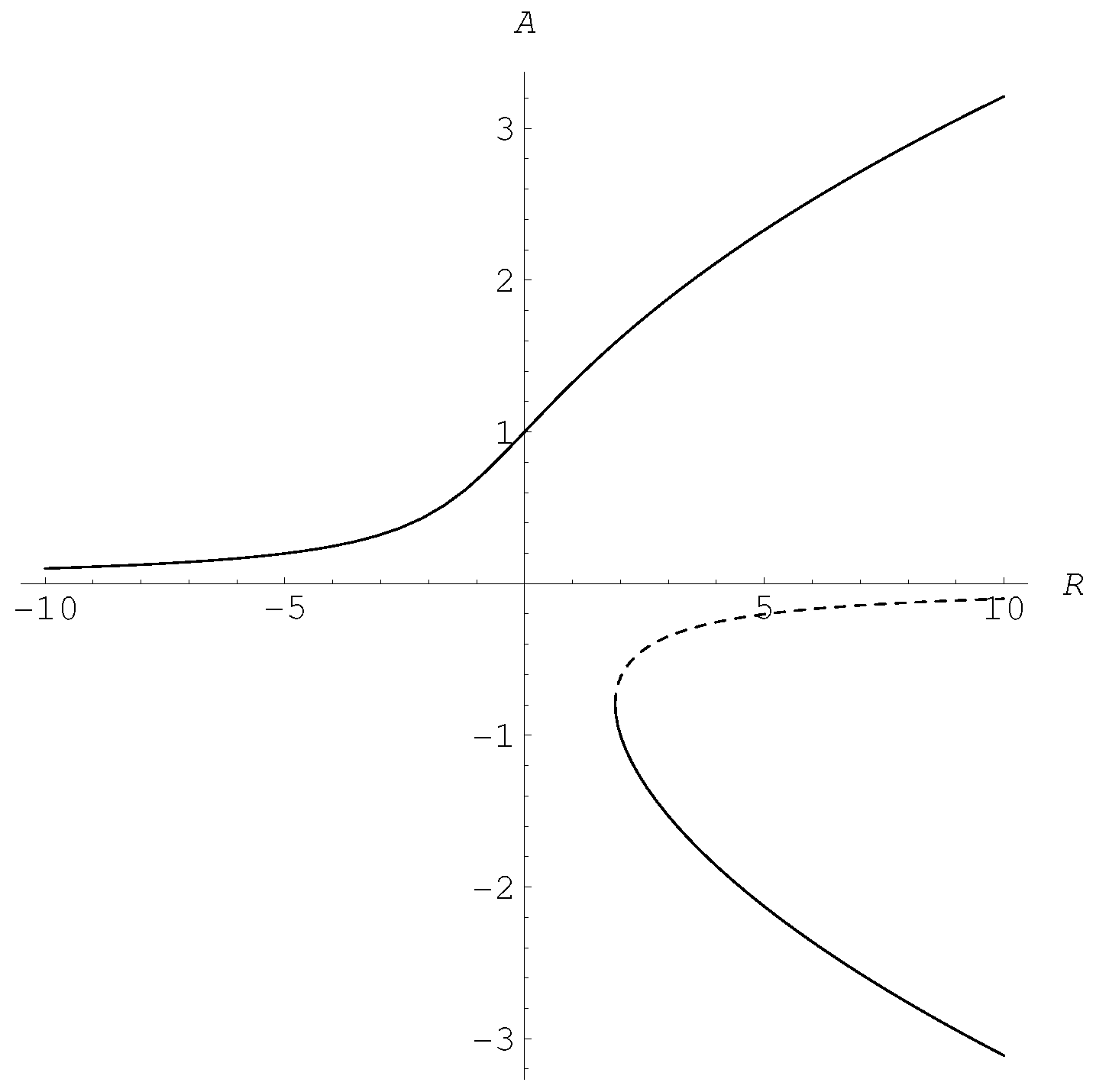
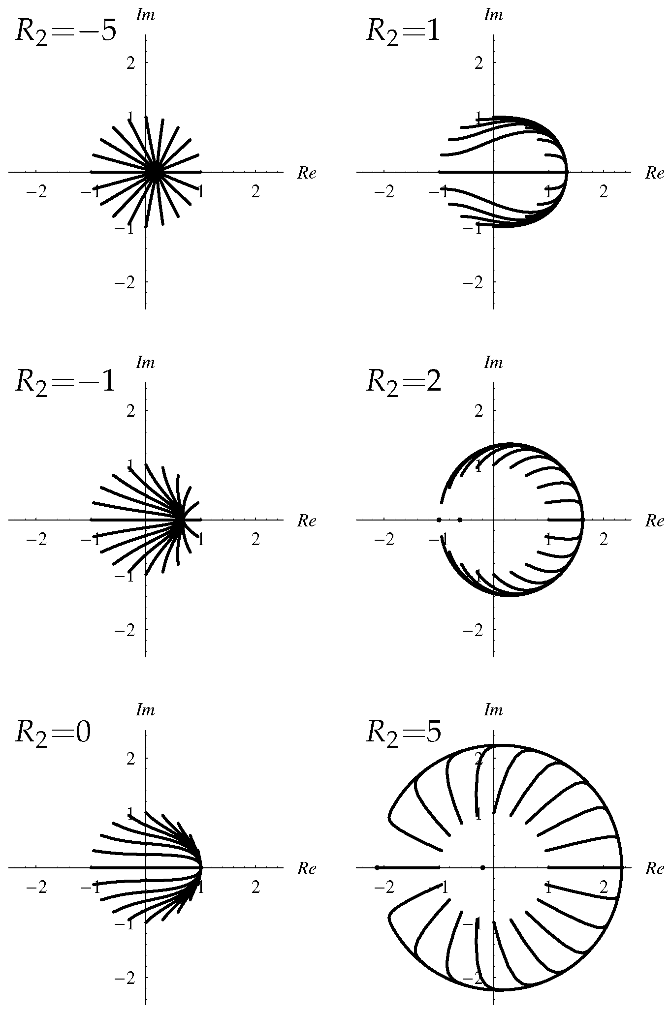
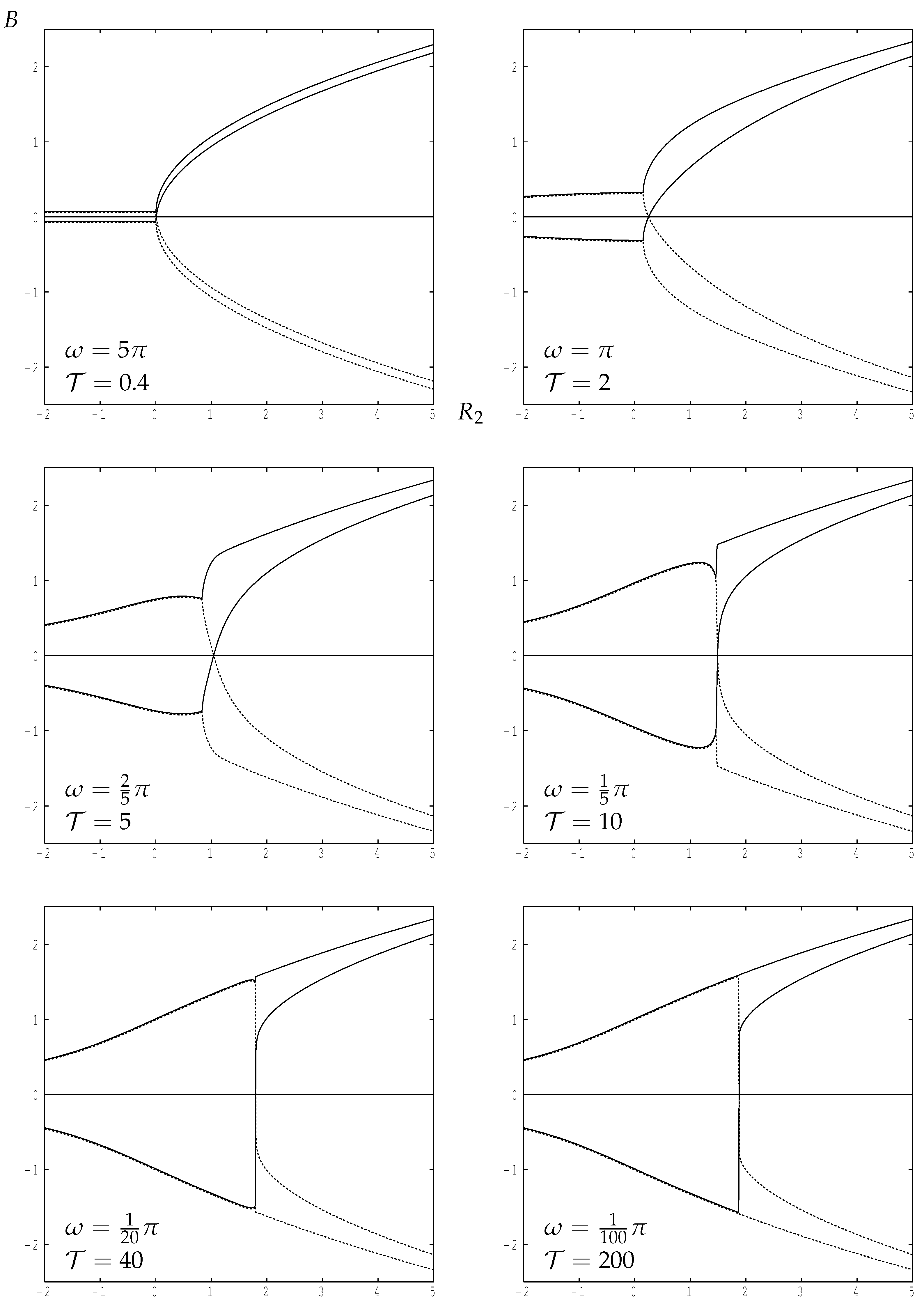
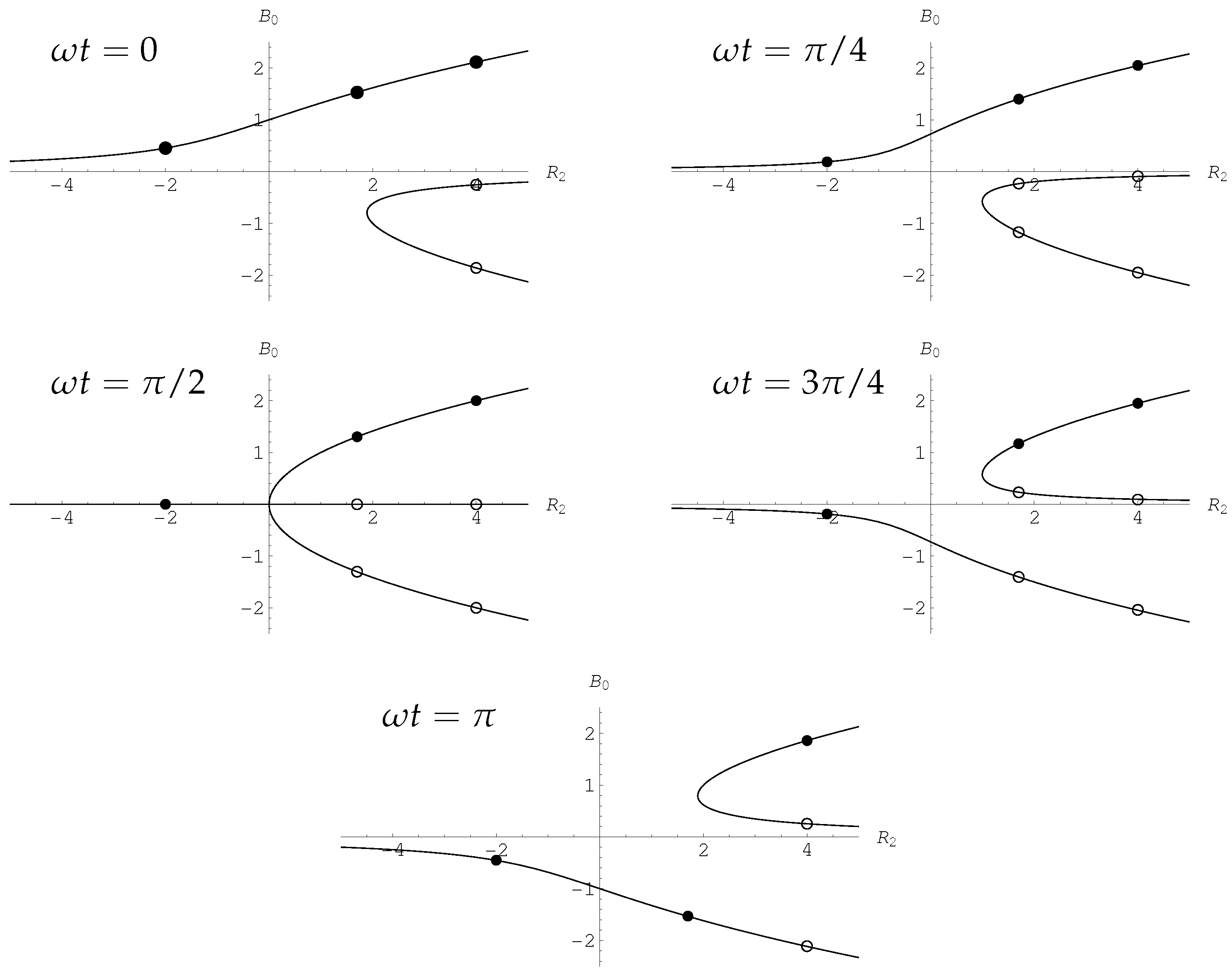
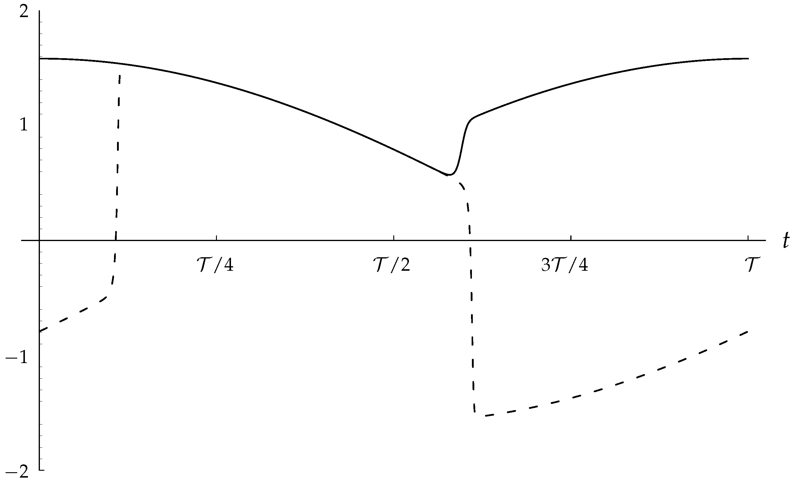
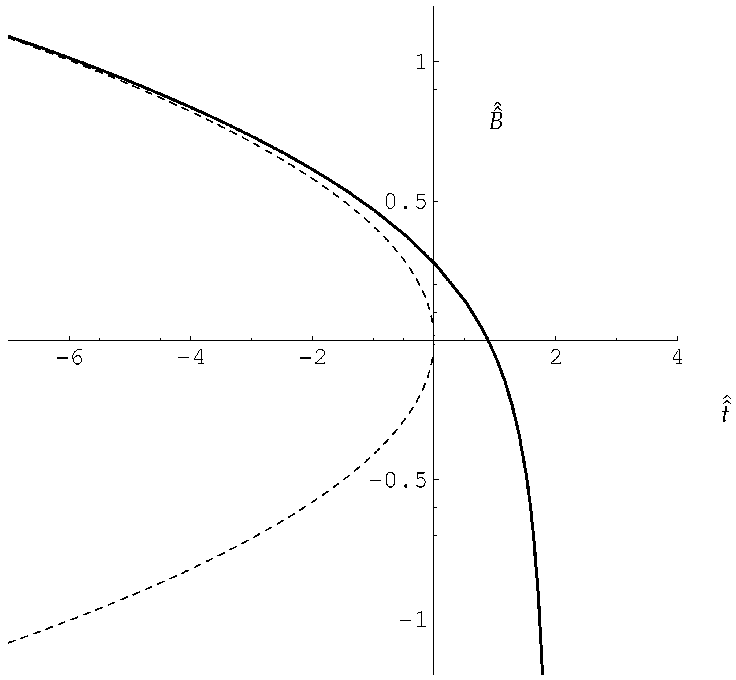
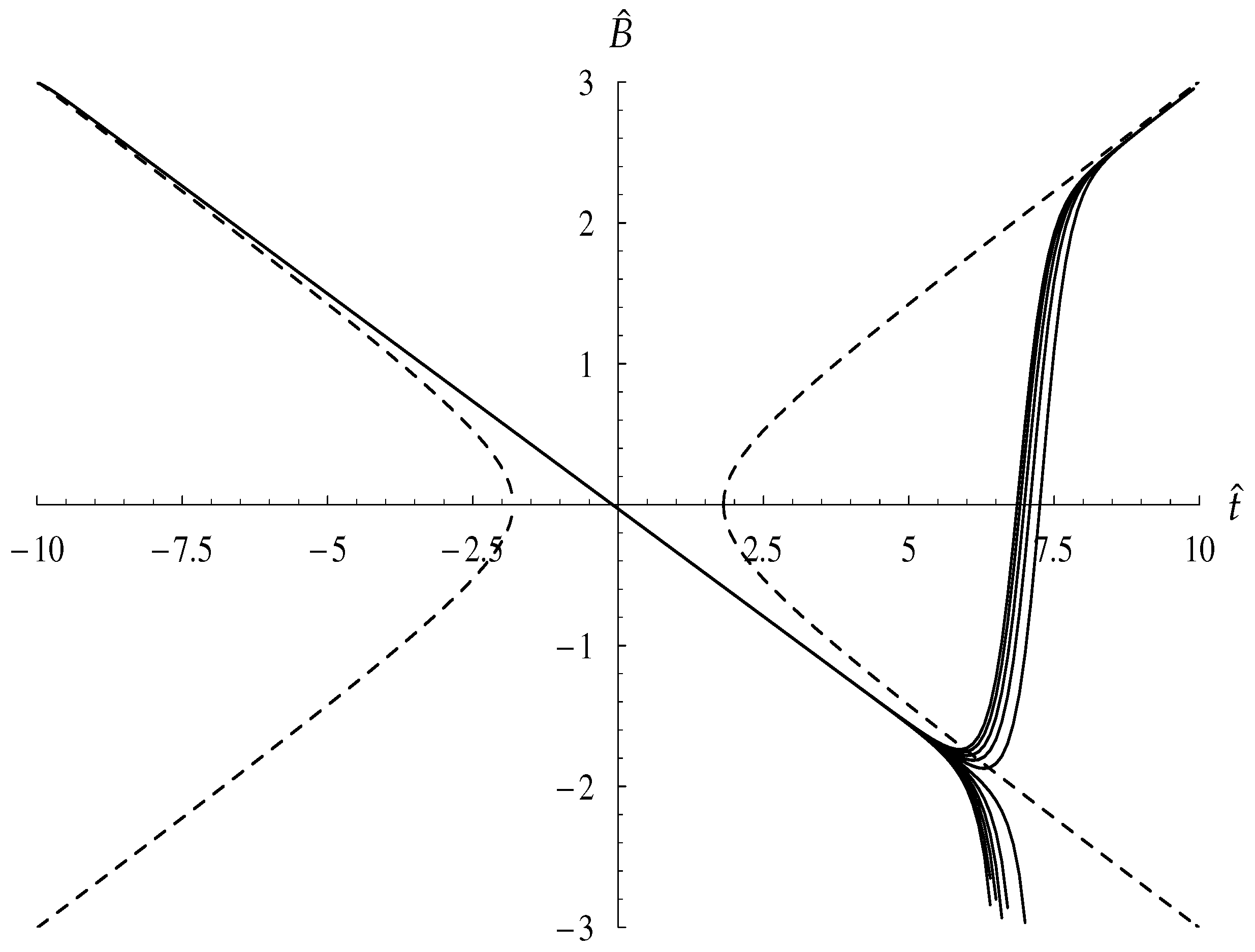
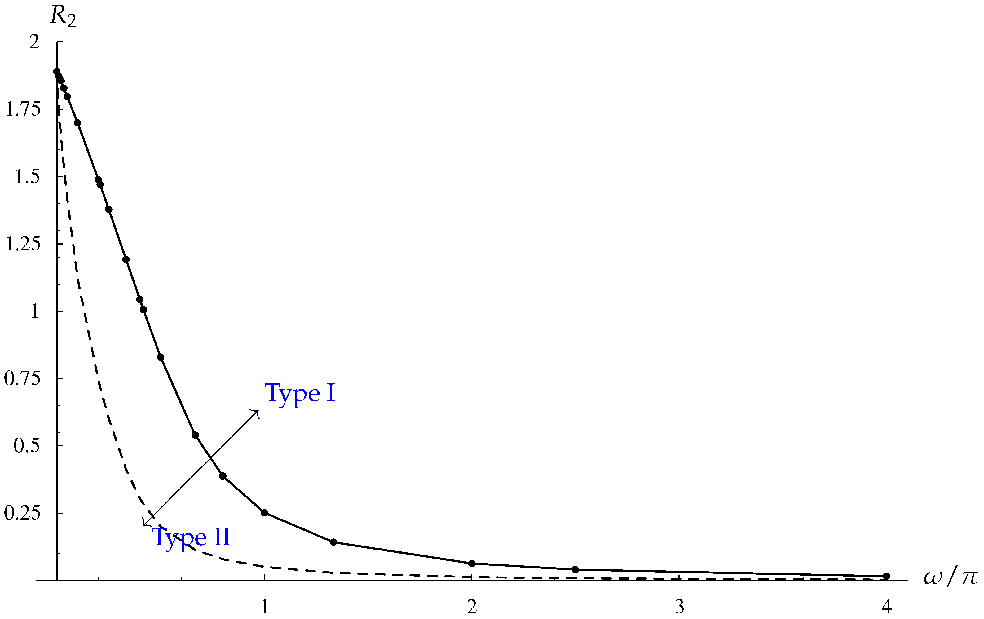
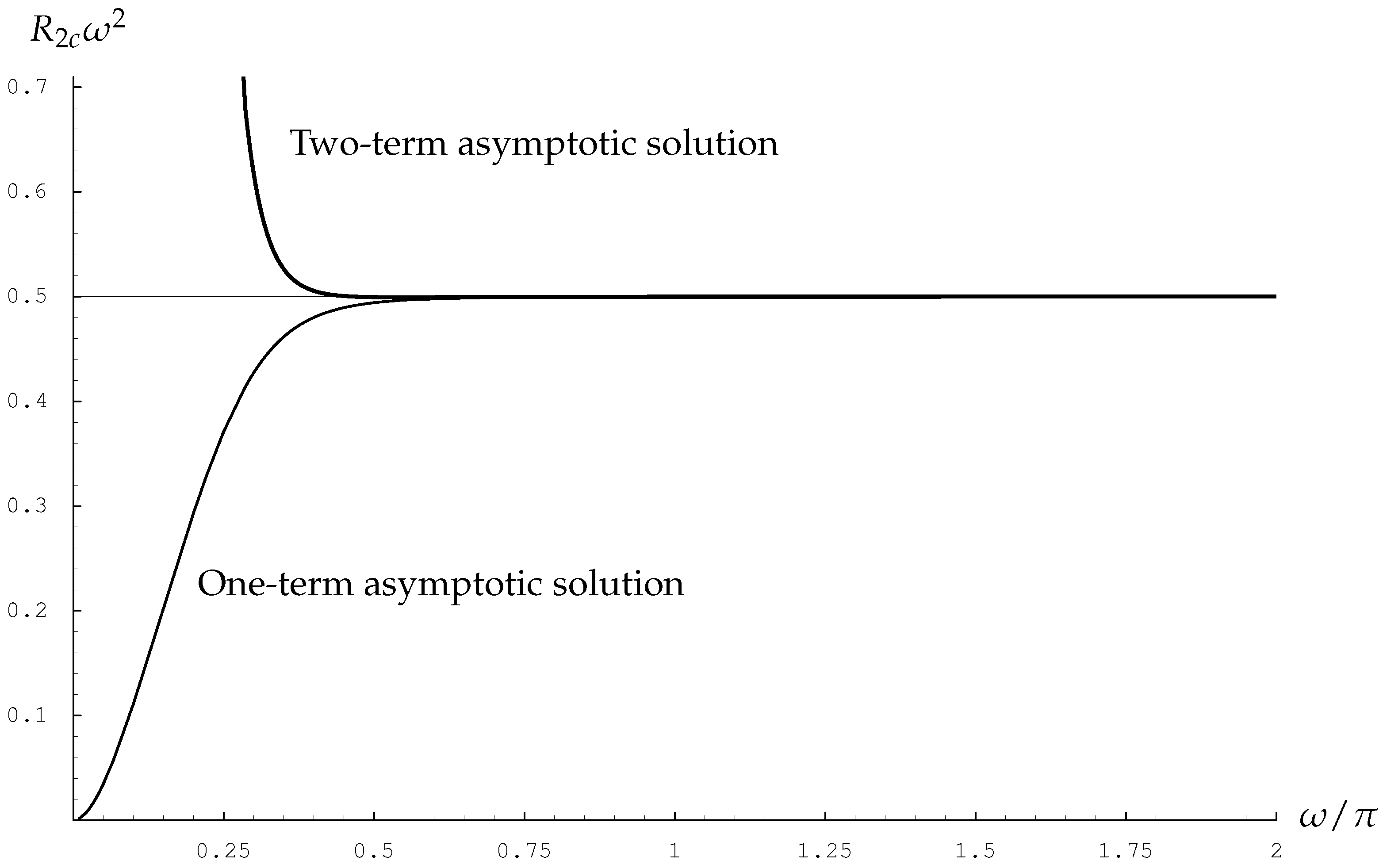
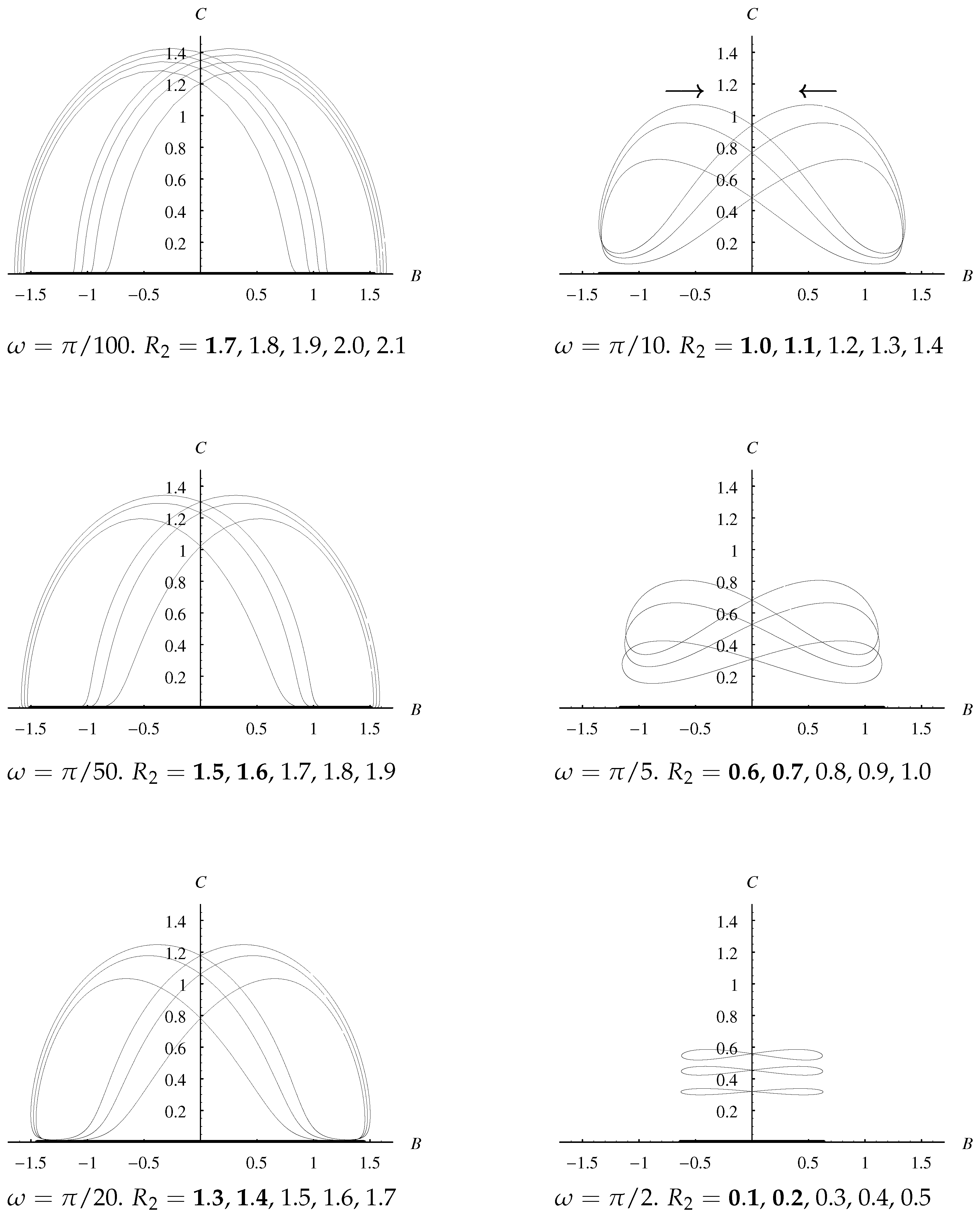
There exist different solutions of this amplitude equation in different regions of Rayleigh number/wavenumber space. If the flow is constrained to be stationary, which will happen if the layer is bounded by suitably-placed sidewalls with impermeable and insulating boundary conditions, then what is termed a Type II flow exists and is stable when R a is below a frequency-dependent critical value. As R a increases there is a supercritical bifurcation to what is termed a Type I flow. Flows of Type II are double-signed, whereas Type I flows are usually single-signed—exceptions are situated close to the bifurcation point. Detailed asymptotic solutions are presented for small frequencies where the numerical solutions display localised and quite rapid changes in sign.
When the layer is unbounded horizontally, then the real-A stationary solutions are susceptible to disturbances in phase, and we find that all Type I solutions are unstable to this type of disturbance. Type II real solutions may also be destabilised if R 2 is sufficiently large to become one with complex amplitude, which corresponds to a convection pattern which oscillates horizontally.
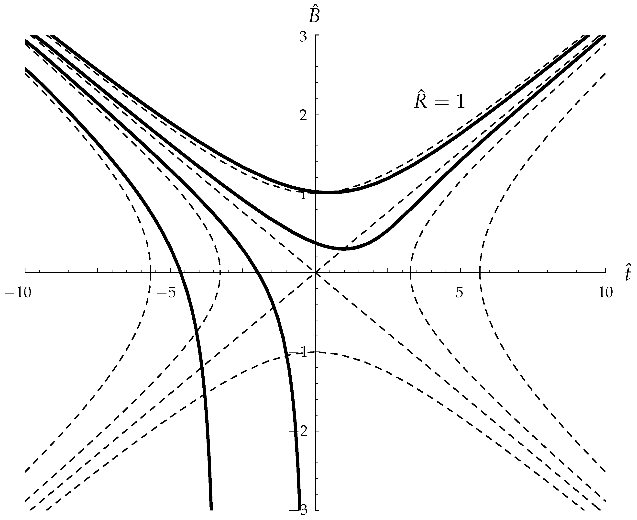
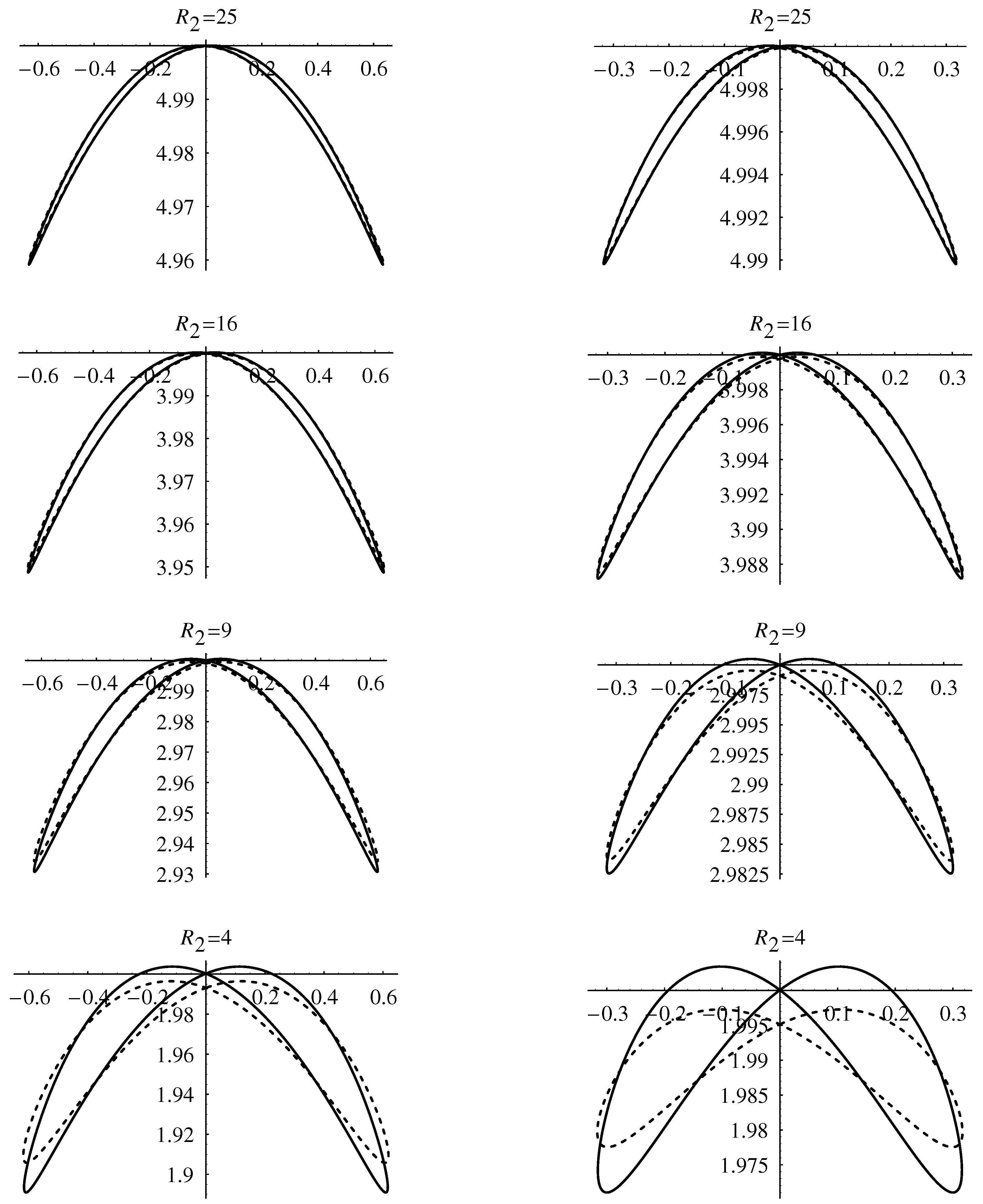
Numerical solutions have in many cases been supplemented by asymptotic solutions and these have shown excellent agreement.
Three dimensional disturbances have not been considered in this paper. Given that the boundary disturbances have a spatial pattern which has the critical wavenumber, it is our a priori expectation that three-dimensional effects are subdominant. However, we think that three-dimensional effects will be important when the spatial wavenumber of the disturbance is different from k = π . Certainly it is the case that such patterns are dominant when these boundary forcing terms are steady in time; see Rees and Riley 1989(a,b) [12].
Finally we note that some of the work described here on moving cells may need to be modified if a layer of long but finite length were to be considered. It has already been stated that disturbances in phase cannot arise in a short layer due to the presence of sidewalls. However, if the layer is of finite but sufficiently large extent (which will be of O ( δ 1 / 3 ) ), then it may well be possible for cells to be compressed slightly near those sidewalls, and this would allow for phase movements in the bulk which then reduce in magnitude as the sidewalls are approached. In these the resulting time-dependent flow may be visualized by having stationary cells fixed or pinned to the two sidewalls, rather than being generated or annihilated, and then the magnitude of the time-variation of the phase of all other cells will increase to a maximum midwall between the sidewalls. If the layer is sufficiently long, then there will be a substantial region in the middle of the layer where the present theory is valid.
It is also intended to extend the present work well into the nonlinear regime.

Acknowledgments

Ibrahim M. Jais would like to thank Universiti Teknologi Malaysia for funding his Ph.D. studies at the University of Bath under the supervision of D. Andrew S. Rees. The authors would like to thank the reviewers for their kind remarks and for some ideas to improve the manuscript.

Author Contributions

The reported research is drawn from the doctoral studies of Ibrahim M. Jais and both authors contributed to the writing of the paper.

Conflicts of Interest

There are no conflicts of interest.

Abbreviations

Aamplitude of convection
Breal part of A
cheat capacity
Cimaginary part of A
dheight of the porous layer
Ddisturbance
ggravity
kwavenumber
Kpermeability
ppressure
RaDarcy-Rayleigh number
R 1 , R 2 Right hand sides of Equations (28) and (29)
ttime
T nondimensional forcning period
Tdimensional temperature
Tcupper (cold) boundary temperature
Thlower (hot) boundary temperature
u,vhorizontal velocities
wvertical velocity
x,yhorizontal coordinates
zvertical coordinate
Greek symbols
βthermal expansion coefficient
δamplitude of thermal imperfection
ϵamplitude of convection
θtemperature
μdynamic viscosity
ρdensity
σheat capacity ratio
τscaled time
ψstreamfunction
ϕporosity
ωfrequency
Subscripts, superscripts, and other symbols
ccritical value
ffluid
ssolid
-dimensional quantity
0, 1, 2, ⋯terms in a series expansion

References

  1. Mojtabi, A.; Rees, D.A.S. The onset of the convection in Horton-Rogers-Lapwood experiments: The effect of conducting bounding plates. Int. J. Heat Mass Transf. 2011, 54, 293–301. [Google Scholar] [CrossRef] [Green Version]
  2. Lapwood, E.R. Convection of a fluid in a porous medium. Proc. Camb. Philos. Soc. 1948, 4, 508–521. [Google Scholar] [CrossRef]
  3. Rees, D.A.S. The stability of Darcy-Bénard convection. In Handbook of Porous Media; Vafai, K., Ed.; Marcel Dekker: New York, NY, USA, 2000; pp. 521–558. [Google Scholar]
  4. Palm, E.; Weber, J.E.; Kvernvold, O. On steady convection in a porous medium. J. Fluid Mech. 1972, 54, 153–161. [Google Scholar] [CrossRef]
  5. Straus, J.M. Large amplitude convection in porous media. J. Fluid Mech. 1974, 64, 51–63. [Google Scholar] [CrossRef]
  6. Horton, C.W.; Rogers, F.T., Jr. Convection currents in a porous medium. J. Appl. Phys. 1945, 16, 367–370. [Google Scholar] [CrossRef]
  7. Tyvand, P.A. Onset of Rayleigh-Bénard Convection in Porous Bodies. In Transport Phenomena in Porous Media II; Pergamon: Oxford, UK, 2002; pp. 82–112. [Google Scholar]
  8. Nield, D.A.; Bejan, A. Convection in Porous Media, 5th ed.; Springer: Berlin, Germany, 2017. [Google Scholar]
  9. Riahi, D.N. Nonlinear convection in a porous layer with finite conducting boundaries. J. Fluid Mech. 1983, 129, 153–171. [Google Scholar] [CrossRef]
  10. Saleh, H.; Saeid, N.H.; Hashim, I.; Mustafa, Z. Effect of conduction in bottom wall on Darcy-Bénard convection in a porous enclosure. Transp. Porous Media 2011, 88, 357–368. [Google Scholar] [CrossRef]
  11. Rees, D.A.S.; Mojtabi, A. The effect of conducting boundaries on weakly nonlinear Darcy-Bénard convection. Transp. Porous Media 2011, 88, 45–63. [Google Scholar] [CrossRef]
  12. Rees, D.A.S.; Riley, D.S. Convection in a porous layer with spatially periodic boundary conditions: Resonant wavelength excitation. J. Fluid Mech. 1986, 166, 503–530. [Google Scholar] [CrossRef]
  13. Rees, D.A.S.; Riley, D.S. The effects of boundary imperfections on convection in a saturated porous layer: Near-resonant wavelength excitation. J. Fluid Mech. 1989, 199, 133–154. [Google Scholar] [CrossRef]
  14. Rees, D.A.S.; Riley, D.S. The effects of boundary imperfections on convection in a saturated porous layer: Non-resonant wavelength excitation. Proc. R. Soc. Lond. 1989, A421, 303–339. [Google Scholar] [CrossRef]
  15. Rees, D.A.S. The effect of long-wavelength thermal modulations on the onset of convection in an infinite porous layer heated from below. Q. J. Mech. Appl. Math. 1990, 43, 189–214. [Google Scholar] [CrossRef]
  16. Vozovoi, L.P.; Nepomnyaschii, A.A. Convection in a horizontal layer in the presence of spatial modulation of the temperature at the boundaries. Gidrodinamika 1974, 8, 105–117. (In Russian) [Google Scholar]
  17. Tavantzis, J.; Reiss, E.L.; Matkowsky, B.J. On the smooth transition to convection. SIAM J. Appl. Math. 1978, 34, 322–337. [Google Scholar] [CrossRef]
  18. O’Sullivan, M.J.; McKibbin, R. Heat transfer in an unevenly heated porous layer. Transp. Porous Media 1986, 1, 293–312. [Google Scholar] [CrossRef]
  19. Riahi, D.N. Preferred pattern of convection in a porous layer with a spatially non-uniform boundary temperature. J. Fluid Mech. 1993, 246, 529–543. [Google Scholar] [CrossRef]
  20. Riahi, D.N. Finite amplitude thermal convection with spatially modulated boundary temperature. Proc. R. Soc. Lond. 1995, A449, 459–478. [Google Scholar] [CrossRef]
  21. Mamou, M.; Robillard, L.; Bilgen, E.; Vasseur, P. Effects of a moving thermal wave on Bénard convection in a horizontal saturated porous layer. Int. J. Heat Mass Transf. 1996, 39, 347–354. [Google Scholar] [CrossRef]
  22. Banu, N.; Rees, D.A.S. The effect of a travelling thermal wave on weakly nonlinear convection in a porous layer heated from below. J. Porous Media 2001, 4, 225–239. [Google Scholar] [CrossRef]
  23. Prats, M. The effect of horizontal fluid motion on thermally induced convection currents in porous mediums. J. Geophys. Res. 1967, 71, 4835–4838. [Google Scholar] [CrossRef]
  24. Dufour, D.; Néel, M.-C. Numerical study of instability in a horizontal porous channel with bottom heating and forced horizontal flow. Phys. Fluids 1998, 10, 2198–2207. [Google Scholar] [CrossRef]
  25. Plapp, B.B.; Egolf, D.A.; Bodenschatz, E. Dynamics and selection of giant spirals in Rayleigh-Bénard convection. Phys. Rev. Lett. 1998, 81, 5334–5337. [Google Scholar] [CrossRef]
  26. Newell, A.C.; Whitehead, J.A. Finite bandwidth, finite amplitude convection. J. Fluid Mech. 1969, 38, 279–303. [Google Scholar] [CrossRef]
Figure 1. Neutral curve for the classical Darcy-Bénard problem with n = 1 ; see Equation (1). the critical values are given by R a c = 4 π 2 and k c = π .
Fluids 02 00060 g001
Figure 2. The steady solution curves for the amplitude equation Equation (37). The upper branch is stable. The other two branches are unstable with respect to perturbations in phase, while the middle branch is also unstable with respect to perturbations in amplitude.
Fluids 02 00060 g002
Figure 3. Numerical solutions of Equation (37) for initial conditions placed on a unit circle in the complex plane, for R a = 5 , 1 , 0, 1, 2 and 5. Showing how solutions evolve to the unique solution on the positive real axis.
Fluids 02 00060 g003
Figure 4. The effect of different Rayleigh numbers on real solutions of Equation (36) for the following selection of forcing periods: T = 1 , 5, 20 and 100. The respective frequencies are ω = 2 π , 0.4 π , 0.1 π and 0.02 π . The uppermost curve corresponds to R 2 = 3 ; the dash-dotted curve to Ra = 0 with intermediate curves corresponding to intervals of 0.2 in R a ; the dotted curves correspond to R a = 1 , 2 , 5 and 10 .
Fluids 02 00060 g004
Figure 5. The bifurcation diagram for the given values frequencies/periods. The curves correspond to B max and B min over period. The dashed lines correspond to solutions for which B ( t = 0 ) is negative, while continuous lines have B ( t = 0 ) > 0 .
Fluids 02 00060 g005
Figure 6. Depiction of the bifurcation diagram corresponding to quasi-static real solutions of Equation (40) over half a period. The five frames correspond to ω t = 0 , π / 4 , π / 2 , 3 π / 4 and π . In each frame, and from left to right, the symbols indicate potential solutions for (i) R 2 < 0 , (ii) 0 < R 2 < 3 / 2 2 / 3 and (iii) R 2 > 3 / 2 2 / 3 . The solid circles depict how one might predict how an unsteady solution might evolve from the initial conditions given when ω t = 0 , while the circles depict possible solutions but these do not arise with the chosen initial conditions.
Fluids 02 00060 g006
Figure 7. An example of a catastrophic change in the qualitative nature of the solution for the small frequency, ω = π / 100 . The solid line corresponds to R 2 = 1.871666 and the dashed line to R 2 = 1.871665 .
Fluids 02 00060 g007
Figure 8. Solution curves (continuous lines) for ω = π / 100 ( T = 200 ) and for R 2 = 1.4 (lowest), 1.8 and 2.0 (uppermost). Also shown are the corresponding quasi-static solutions.
Fluids 02 00060 g008
Figure 9. Solution of Equation (66) for S = 0.5 (continuous line). The corresponding quasi-static solution of 3 B ^ ^ 2 = S t ^ ^ is represented by the dashed line.
Fluids 02 00060 g009
Figure 10. Solution of Equation (73) for R ^ = 0.3 , 1 , 0 and 1 (continuous lines). The corresponding quasi-static solutions are represented by the dashed lines.
Fluids 02 00060 g010
Figure 11. Solutions of Equation (73) for values of R ^ which are close to the critical value, i.e., R ^ = 0.3054955 ± n × 10 7 with n = 5 , 4 , , 4 , 5 (continuous lines). The corresponding quasi-statics solution is represented by the dashed line.
Fluids 02 00060 g011
Figure 12. Showing the value of R 2 as a function of ω at which solutions of Type II undergo a supercritical bifurcation to solutions of Type I (continuous line), and the neutral stability curve with respect to imaginary disturbances (dashed line).
Fluids 02 00060 g012
Figure 13. Critical values of R 2 above which real solutions are unstable to iaginary disturbances (dashed line). Also shown are one-term (thin line) and two-term (thick line) approximations using a large- ω analysis.
Fluids 02 00060 g013
Figure 14. The effect of different values of R 2 and ω on solution trajectories. Bold values of R 2 indicate values for which solutions are real. All solution trajectories follow that of the arrow shown in the top right subfigure.
Fluids 02 00060 g014
Figure 15. Continuous curves show the solution trajectories for the given values of R 2 . The left hand column corresponds to ω = π / 2 and the right hand column corresponds to ω = π / 20 . Dashed lines indicate the large- R 2 asymptotic solution.
Fluids 02 00060 g015
Table 1. The values of R 2 corresponding to the transition between Type I and Type II solutions of Equation (40). R 2 zero marks where B min = 0 , while R 2 bif marks the bifurcation point in Figure 5.
ω / π R 2 zero R 2 bif
0 1.889881 1.889881
1/100 1.871665 1.871665
1/50 1.853286 1.853286
1/20 1.797093 1.797080
1/10 1.699355 1.699006
1/5 1.488797 1.466053
1/4 1.378595 1.321533
1/3 1.192159 1.050448
2/5 1.043338 0.837670
1/2 0.829189 0.583587
2/3 0.540125 0.339267
4/5 0.388046 0.236835
1 0.251850 0.151874
4/3 0.142320 0.085479
2 0.063326 0.037995
4 0.015856 0.009499
Table 2. Numerical solutions showing the relationship between ω and R 2 c corresponding to neutral stability with respect to phase perturbations. In the right hand subtable we also show R 2 c , asymp from Equation (92) and its error.
ω / π R 2 c
01.88988158
0.0011.84449388
0.0021.83042922
0.0051.79452727
0.011.74209700
0.021.64886998
0.051.41741816
0.11.12923353
0.20.74433223
0.30.56289546
ω / π R 2 c R 2 c , asymp R 2 c R 2 c , asymp
0.40.304101420.30211086 1.99 × 10 3
0.50.200307540.20020688 1.01 × 10 4
0.60.140165560.14015740 8.16 × 10 6
0.80.079100610.07910046 1.48 × 10 7
10.050651080.05065108 7 × 10 9
1.50.022515450.02251545
20.012665110.01266511
30.005628950.00562895
50.002026420.00202642
100.000506610.00050661

