Investigation of the Turbulent Near Wall Flame Behavior for a Sidewall Quenching Burner by Means of a Large Eddy Simulation and Tabulated Chemistry

Abstract

Combustion will play a major part in fulfilling the world’s energy demand in the next 20 years. Therefore, it is necessary to understand the fundamentals of the flame–wall interaction (FWI), which takes place in internal combustion engines or gas turbines. The FWI can increase heat losses, increase pollutant formations and lowers efficiencies. In this work, a Large Eddy Simulation combined with a tabulated chemistry approach is used to investigate the transient near wall behavior of a turbulent premixed stoichiometric methane flame. This sidewall quenching configuration is based on an experimental burner with non-homogeneous turbulence and an actively cooled wall. The burner was used in a previous study for validation purposes. The transient behavior of the movement of the flame tip is analyzed by categorizing it into three different scenarios: an upstream, a downstream and a jump-like upstream movement. The distributions of the wall heat flux, the quenching distance or the detachment of the maximum heat flux and the quenching point are strongly dependent on this movement. The highest heat fluxes appear mostly at the jump-like movement because the flame behaves locally like a head-on quenching flame.

1. Introduction

The world’s primary energy demand will be increasing about 30% in the next 20 years, and 75% of this demand will be provided by combustion [1,2]. Since resources are limited and combustion can cause pollution, it is necessary to better understand the fundamentals. One important field, in which research is required, is the flame–wall interaction (FWI). Due to technical improvements, e.g., of internal combustion engines or gas turbines, its relevance rises [3,4]. Here, the reaction zone of the flame gets close to cold walls and quenches. This reduces efficiencies and increases pollution formation [5]. The FWI can be subdivided into two canonical configurations, namely head on quenching (HOQ) and sidewall quenching (SWQ) [5]. In the latter case, the flame moves perpendicular along the wall and only the flame tip is affected. In case of HOQ, the flame moves parallel towards the wall and the whole flame quenches. The dimensionless quantities for the quenching distance and heat flux differ clearly in both cases. Because of the importance of the FWI, an SWQ configuration is considered in this work.

In terms of premixed conditions, SWQ has been widely studied theoretically, experimentally and numerically. Primarily, fuels like hydrogen and gaseous hydrocarbons, such as methane, ethylene, propane or butane, were used. The most simple fuel, but experimentally difficult to handle, is hydrogen. It was investigated by Cheng et al. [6] for an experimental turbulent boundary layer over a heated wall. They determined the limits of the reactions near the wall depending on the equivalence ratio. A more recent study regarding hydrogen combustion was conducted by Gruber et al. [7]. Within their three-dimensional direct numerical simulation (DNS), the authors used detailed chemistry (DC). Their data suggests that near-wall coherent turbulent structures are important for the wall heat flux and that the heat release rate at the wall is strongly controlled by exothermic radical recombination reactions. However, hydrogen behaves differently than hydrocarbon based fuels because it has a much higher consumption speed and it will not be investigated in this current work.

The effect on the quenching layer thickness of different hydrocarbons with variations in the equivalence ratio and different wall conditions was researched by Saffman [8]. The investigations of Lu et al. [9] and Ezekoye et al. [10] used different fuels and equivalence ratios as well, but in a constant volume chamber. They measured the unsteady heat transfer during SWQ. Boust et al. [11] developed a thermal formulation for single-wall quenching without any empirical coefficients. This formulation is based on experimental data and is applicable for lean and stoichiometric methane/air mixtures in a pressure range from 0.05–0.35 MPa. DNS studies combined with a single step mechanism, which mimics a lean methane flame with an inlet temperature of 600 K were carried out by Alshaalan and Rutland [12,13]. They investigated a V-shaped flame in a weakly turbulent Couette flow. Nevertheless, the number of simulations with a chemistry treatment beyond single step mechanisms for hydrocarbons is sparse and most turbulent premixed FWI investigations were focused on the HOQ configuration.

In the present numerical study, an SWQ burner configuration is investigated, which is based on the experimental design of Jainski et al. [14,15]. In the experimental setup, a premixed V-shaped flame interacts with a cooled wall under laminar and turbulent conditions. First numerical results for both cases have been already provided by Heinrich et al. [16,17] with a highly-resolved (large eddy simulation) LES with DNS-like spatial resolution. The turbulent and laminar cases were compared and analyzed with each other and the experiments. The global structure of the flame, the flame position, the temperature field and the velocities are given correctly by the methods used. Compared to other highly resolved simulations [7,12,13], which used simple configuration, this setup is more complex and the turbulent structures of the flow are not comparable with channel or pipe flows. In this work, a transient analysis of the flame–wall–turbulence interaction (FWTI) is conducted. This gives further insight into heat fluxes, quenching distances and quenching positions beyond the experimental findings. It will be shown that a strong dependency of the moving direction of the flame tip for characteristic properties exist. Moreover, it will be explained that the highest heat fluxes occur because the turbulent SWQ flame behaves locally like an HOQ flame.

The remainder of the paper is structured as follows: the numerical description, the chemistry treatment and the domain are given in Section 2. The transient analysis of the FWI is provided in Section 3. Finally, conclusions are given in Section 4.

2. Methods

2.1. Numerical Description

The simulation in this work has been conducted with the Finite Volume code FASTEST. It is a block-structured code that uses hexahedral, boundary fitted grids to represent complex geometries. The Massage Passing Interface (MPI) is utilized for the inter-processor communication. The incompressible Favre-averaged Navier–Stokes equations with a low-Mach number formulation for the variable density $\rho$ are discretized with a second order spacial scheme [18] and the time integration is done by an explicit low storage three-stage Runge–Kutta scheme with second order accuracy. In each Runge–Kutta step, the pressure correction procedure is applied. The corresponding mass and momentum equations are the following:

$$\begin{array}{cc}\hfill {\displaystyle \frac{\partial \overline{\rho }}{\partial t}}+{\displaystyle \frac{\partial }{\partial x_i}}\left(\overline{\rho }{\tilde{u}}_i\right)& =0\hfill \end{array}$$

(1)

$$\begin{array}{cc}\hfill {\displaystyle \frac{\partial }{\partial t}}\left(\overline{\rho }{\tilde{u}}_j\right)+{\displaystyle \frac{\partial }{\partial x_i}}\left(\overline{\rho }{\tilde{u}}_i{\tilde{u}}_j\right)& ={\displaystyle \frac{\partial }{\partial x_i}}\left({\overline{\tau }}_{ij}-\overline{\rho }{\tau }_{sgs}\right)-{\displaystyle \frac{\partial \overline{p}}{\partial x_j}}+\overline{\rho }{g}_j\hfill \end{array}$$

(2)

The quantity u is the velocity, p is the pressure, ${\tau }_{ij}$ is the shear stress tensor and the operators $\tilde{}$ and $\overline{}$ represent the Favre-averaging and filtering operation, respectively. The sub grid fluxes of the momentum ${\tau }_{sgs}$ are accounted by eddy viscosity approach proposed by Smagorinsky [19]. The model coefficient is determined by the dynamic procedure proposed by Germano et al. [20] with a modification by Lilly [21]. For the discretization of the convective terms in the scalar transport equations, a total variation diminishing (TVD) limiter as proposed by Zhou et al. [22] is used.

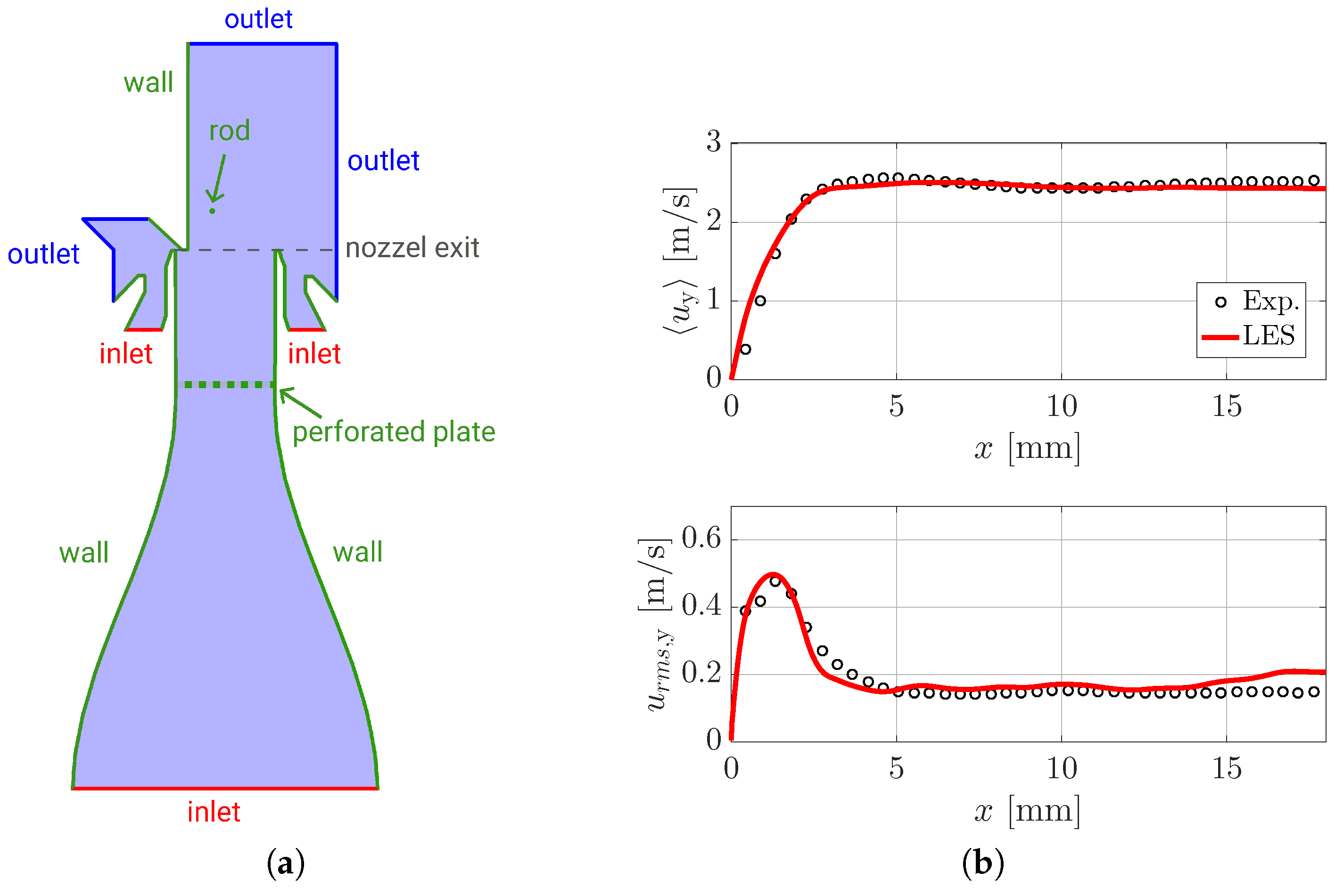
2.2. Numerical Domain

Figure 1 displays the numerical domain used in this work, which is based on the experimental setup of Jainski et al. [14]. The dimensions are given on the left side of this figure. On the right side, an instantaneous velocity field of the center plane with the flame front is shown in the three-dimensional domain. The turbulent inlet flow and acceleration of the fluid due to the flame front is clearly visible.

Like in the experiments [14], the wall temperature is kept constant at $T_w=350$K and the rod temperature is set to 300 K. The numerical rod is fully resolved with an O-grid. To stabilize the stoichiometric methane main flow, it is surrounded by a pure air co-flow (see Figure 1a). The inlet temperatures of the main and co-flow are 300 K. The turbulent inlet flow was calculated in a pre-processing step by simulating the experimental burner geometry. Each time step, a turbulent velocity field is set at the inlet. How this was calculated will be explained in the next paragraph. At the outlets, convective boundary conditions are used. A block structured grid with approximately 21.5 million control volumes is applied. Distant from the wall, the spatial resolution ranges from 200 $\mathsf{\mu }$m to 400 $\mathsf{\mu }$m. Towards the wall, the mesh is refined to 90 $\mathsf{\mu }$m. As discussed in [17] this grid leads to an direct numerical simulation (DNS)-like spatial resolution and no additional wall modeling is needed.

The complete validation and verification of the simulation of the non-reacting turbulent inlet flow can be found in Heinrich et al. [17]. Here, the basic idea will be pointed out. Therefore, the body of the experimental burner was simulated (Figure 2a) and the experimental mass flows for the main and co-flow were set as inlet conditions [14].

The simulated geometry includes the main and co-flow, the perforated plate, the flame stabilizing rod and the wall. The height of the nozzle exit is marked in Figure 2a. The velocity fields were extracted along this area for each time step and stored in a database. Within the burner, the turbulence was generated by the perforated plate. After the nozzle exit, a boundary layer developed at the wall. The Reynolds number based on the nozzle exit is $Re=5300$. The resulting turbulent intensity at the nozzle exit section is approximately $8\%$. The analyses of the flow field revealed that the structures are inhomogeneous. In Figure 2b, the time averaged velocity and its rms-value are shown for the main component 11 mm downstream the nozzle exit. Both quantities are in very good agreement with the experimental values, since the maximum difference between the profiles is less than 0.18 m/s.

2.3. Chemistry Treatment

Depending on the quantities of interest, a very detailed description of the near-wall chemistry may be required. However, the application of full reaction mechanisms, typically covering tens of species and hundreds of elementary reactions, is not possible in complex configurations. Even for the laboratory scale system considered here, the computational cost given by the resolution requirement, the number of transported scalars and their stiff coupling prohibit its application. Accordingly, a chemistry reduction approach by means of tabulation is employed. In the framework of the Flamelet Generated Manifolds (FGM) approach introduced by van Oijen and de Goey [23], pre-computed detailed chemistry solutions of premixed flames enter the chemistry database. By that, vital information is included such that important quantities like the flames’ propagation speed or its spatial structure including all species can be exactly reproduced by means of the controlling variables. The table generation, its assessment in a FWI situation, and its treatment in turbulent flow are briefly outlined in the following.

2.3.1. Construction of the FGM Table

A three-dimensional chemistry table is used where the physical processes of this configuration being the reaction, the heat transfer to the wall and the mixing with the co-flowing air are accounted for by a reaction progress variable $Y_{C{O}_2}$ (being the mass fraction of CO${}_2$), the enthalpy h, and the mixture fraction Z, respectively. The table is illustrated in Figure 3b where the temperature and equivalence ratio have been chosen as the axis for illustrative purposes. As shown on the left, first a slice is generated by joining flamelets obtained with the GRI3.0 reaction mechanism [24,25] for different enthalpy levels. Hereby, region a) can be covered using different preheating temperatures while the burner stabilized method [26] is utilized in region b) where chemical reactions evolve under significant heat losses as present at the wall. Finally, in region c), the absence of activation energy suppresses most of the chemical activity and it mostly corresponds to a cooling of exhaust gases. Accordingly, the thermo-chemical states in this region can no longer be obtained by detailed chemistry simulations and Ketelheun et al. [27] approximated them by a thermo-dynamically consistent extrapolation. To cover mixing (i.e., different equivalence ratios), several of those slices are then combined to build the final three-dimensional table as given on the right of Figure 3b. Here, the source term ${\dot{\omega }}_{{\mathrm{CO}}_2}$ has been added representing one of the quantities extracted during the lookup in the simulation.

2.3.2. Evaluation of Simplifying Assumptions for FWI Application

The above-mentioned tabulation approach has been successfully applied to turbulent laboratory scale combustors [28,29,30] where the FWI is not a crucial part of the physics. With respect to the latter, some works have been conducted to evaluate the accuracy of FGM near cold walls. Specifically, Meier et al. [31] and Ganter et al. [32] performed comparisons to detailed chemistry simulations. It turned out that FGM can generally satisfactorily predict the flame attachment position and the transported major species as well as the temperature profiles. Pollutants such as the accumulation of carbon-monoxide near the wall could not be predicted by FGM (Ganter et al. [33]). They showed that this is also possible by advanced or at least more specific tabulation techniques, which, however, require further development. Based on the analysis, we consider that the FGM approach is sufficiently accurate for the quantities analyzed in this study.

Specific for this work and the assumptions made, Figure 4 shows the evaluation of the employed FGM in a generic, two-dimensional SWQ configuration. Detailed chemistry simulations represent the verification basis for the tabulation in general and also to justify diffusivity assumptions. Regarding the latter, within the table generation, the unity Lewis number assumption is employed, since it simplifies the mapping process due to having a constant enthalpy and mixture fraction throughout a flamelet. The under prediction of the flame speed caused by this assumption (about 30% for the relevant conditions) is then corrected afterwards by consistently altering the chemical sources and diffusivities which accelerates the flame according to classical flame theories [34] while preserving its structure [35].

First, Figure 4a shows the temperature field in the region around the quenching point for orientation. Added to this graphs are lines marking the flame by means of an isothermal as well as the chemical source term obtained by three different simulations. The first (dashed line) is a detailed chemistry simulation employing individual diffusivities for all species and can be considered as the most accurate physical description. The Second (solid line) is also a detailed chemistry simulation but with the Le = 1 assumption. Finally, the dotted line is the FGM solution. Due to the above-mentioned correction of the flame speed, the flame–wall attachment points and flame angles are in close agreement. Slightly upstream of the quenching point (coordinate zero) the individual diffusivities cause the flame to reach slightly closer to the wall while the FGM solution is close to the $Le=1$ detailed chemistry indicating that these deviations are due to the remaining transport simplifications. Downstream of the quenching point, the isothermal of the detailed chemistry simulations then approach each other while the FGM slightly depart from them. Accordingly, and as also analyzed by Ganter et al. [33], this is due to tabulation assumption regarding diffusive fluxes orthogonal to the controlling variables. As mentioned, correcting this would require an immensely increased tabulation effort being currently not yet applicable to this configuration. Considering the rather small errors this seems acceptable. A quantification of the temperature and species evolution is furthermore provided on the right of Figure 4 where profiles are shown extracted along the horizontal lines added on to the left of Figure 4. Here, the blue, magenta and black lines represent the states at the quenching point and one millimeter up- and downstream of it. All of these positions being in the region of intense FWI confirm a very good approximation by the FGM approach for the purpose of this work.

2.3.3. Treatment in the Turbulent FWI Flow

As mentioned above, the thermo-chemical state is described with three transported quantities, the mixture fraction Z, the reaction progress variable $Y_{pv}$ and the enthalpy h:

$$\begin{array}{cc}\hfill {\displaystyle \frac{\partial \overline{\rho }\tilde{Z}}{\partial t}}+{\displaystyle \frac{\partial }{\partial x_j}}\left(\overline{\rho }{\tilde{u}}_j\tilde{Z}\right)& ={\displaystyle \frac{\partial }{\partial x_j}}\left(\left(\mathcal{F}\mathcal{E}{\displaystyle \frac{\overline{\mu }}{Sc}}+(1-\Omega ){\displaystyle \frac{{\mu }_t}{S{c}_t}}\right){\displaystyle \frac{\partial \tilde{Z}}{\partial x_j}}\right)\hfill \end{array}$$

(3)

$$\begin{array}{cc}\hfill {\displaystyle \frac{\partial \overline{\rho }{\tilde{Y}}_{\mathrm{pv}}}{\partial t}}+{\displaystyle \frac{\partial }{\partial x_j}}\left(\overline{\rho }{\tilde{u}}_j{\tilde{Y}}_{\mathrm{pv}}\right)& ={\displaystyle \frac{\partial }{\partial x_j}}\left(\left(\mathcal{F}\mathcal{E}{\displaystyle \frac{\overline{\mu }}{Sc}}+(1-\Omega ){\displaystyle \frac{{\mu }_t}{S{c}_t}}\right){\displaystyle \frac{\partial {\tilde{Y}}_{\mathrm{pv}}}{\partial x_j}}\right)+{\displaystyle \frac{\mathcal{E}}{\mathcal{F}}}{\dot{\omega }}_{\mathrm{pv}}\hfill \end{array}$$

(4)

$$\begin{array}{cc}\hfill {\displaystyle \frac{\partial \overline{\rho }\tilde{h}}{\partial t}}+{\displaystyle \frac{\partial }{\partial x_j}}\left(\overline{\rho }{\tilde{u}}_j\tilde{h}\right)& ={\displaystyle \frac{\partial }{\partial x_j}}\left(\left(\mathcal{F}\mathcal{E}{\displaystyle \frac{\overline{\mu }}{Sc}}+(1-\Omega ){\displaystyle \frac{{\mu }_t}{S{c}_t}}\right){\displaystyle \frac{\partial \tilde{h}}{\partial x_j}}\right),\hfill \end{array}$$

(5)

where $\mu$ is dynamic viscosity, Sc the Schmidt number, $\mathcal{F}$ the thickening factor, $\mathcal{E}$ the efficiency function, $\Omega$ the flame sensor and ${\dot{\omega }}_{\mathrm{pv}}$ the reaction source term. To capture the flame–turbulence interaction correctly, the artificially thickened flame (ATF) approach is used. In this context, the flame has been thickened with $\mathcal{F}$ to resolve its structure on the LES grid. Therefore, the transformation of Butler and O’Rouke [36] is used, where the flame speed is preserved. A dynamic version of the procedure based on a sensor $\Omega$ is used in this work [37,38]:

$$\begin{array}{cc}\hfill \mathcal{F}& =1+({\mathcal{F}}_{max}-1)\Omega ,\hfill \end{array}$$

(6)

$$\begin{array}{cc}\hfill \Omega & =16{\left(Y_{\mathrm{n},\mathrm{pv}}(1-Y_{\mathrm{n},\mathrm{pv}})\right)}^2,\hfill \end{array}$$

(7)

where ${\mathcal{F}}_{max}$ is the grid depending maximum thickening factor and $Y_{\mathrm{n},\mathrm{pv}}$ is the normalized progress variable:

$$\begin{array}{c}\hfill Y_{\mathrm{n},\mathrm{pv}}=\frac{Y_{\mathrm{pv}}-Y_{\mathrm{pv},\min }}{Y_{\mathrm{pv},\max }-Y_{\mathrm{pv},\min }}.\end{array}$$

(8)

Due to the small thickening factor ${\mathcal{F}}_{max}$ of 1.4 in this work, the flame turbulence interaction is only slightly altered. Since ATF is used for the flame–turbulence interaction, the turbulent diffusion is switched of in the region of the flame. As explained in [16], the influence of the dynamic thickening on relevant quantities, like wall heat flux, the flame position and quenching point determination is negligible because the thickening can be retransformed. In general, the interaction with the turbulence is reduced if the flame is artificially thickened. To compensate these effects, Colin [35] used a so-called efficiency function $\mathcal{E}$. The formulation of the implemented efficiency function $\mathcal{E}$ can be found in Charlette et al. [39]. Within this work, $\mathcal{E}$ is nearly negligible because the grid resolution is fine enough and ${\mathcal{F}}_{max}$ is relatively small. Following the classical turbulent premixed combustion diagram from Peters [40], this setup operates in the wrinkled flamelet regime, meaning that the inner flame structure is close to a laminar flame and the thin flame front is wrinkled by the turbulent motion due to the fact that the flamelet concept is valid [40]. Additionally, the effects of curvature and stretch on the mass burning rate have been investigated for the thin reaction zone regime [41] and the corrugated flamelet regime [42]. The resulting errors have been found to be within 5% when using a single progress variable as done in this work. Therefore, FGM can be applied for the considered configuration.

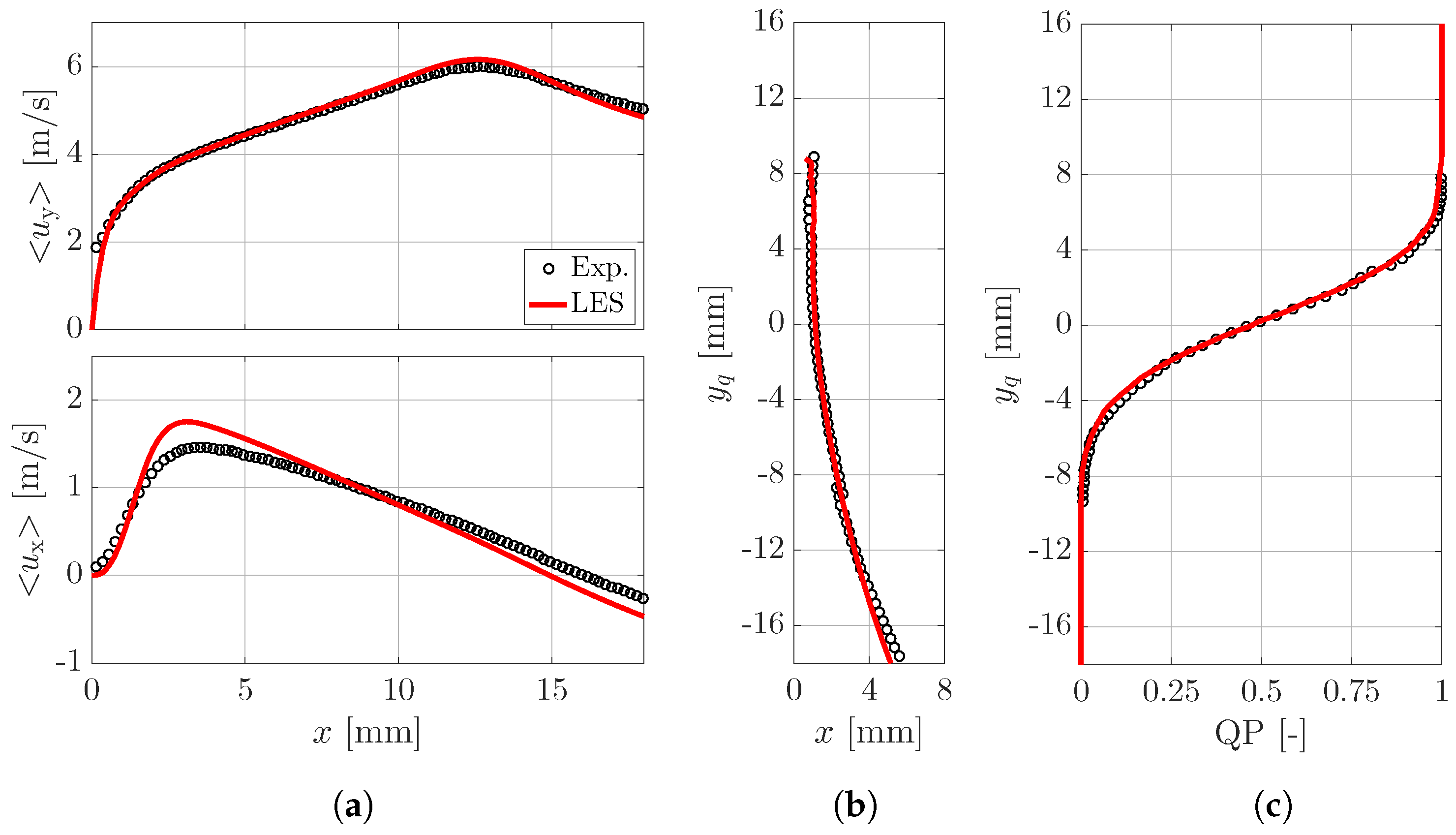
2.4. Determination of the Quenching Point

Following Heinrich et al. [16], the quenching point $y_{qp}$ is determined by tracking the maximum value of the CO${}_2$ source term, which defines the flame front. Due to the enthalpy losses at the wall, this source term decreases and if it drops under a certain threshold the flame is quenched. The threshold is defined as the half of the maximum CO${}_2$ source term along the flame front. This procedure is analogous to the experimental determination where the OH gradient was used. For this FGM approach, using the CO${}_2$ source term is validated against detailed chemistry simulations and it appears to be the most reliable method [16].

2.5. Comparison with Experimental Data

As mentioned before, the models used lead to good results compared to the experimental laminar and turbulent SWQ burner. This was shown before by Heinrich et al. [16,17]. Within these references, the comparisons of the laminar and turbulent for the non-reacting and reacting configurations can be found. For the analyses conducted in Section 3, the velocity, flame position and quenching points are of importance. For the sake of completeness, these quantities are shown again in Figure 5.

Firstly, a conditioned coordinated system has to be introduced ($x_{\mathrm{q}}$, $y_{\mathrm{q}}$) with respect to local averaged quenching point is introduced. It is centered at the wall with $x_{\mathrm{q}}$ = 0 mm and $y_{\mathrm{q}}$ = 0 at the averaged axial quenching point (exemplary marked with the black solid circles in Figure 6). The experimental data is taken from Jainski et al., 2016 [14]. The velocity profiles 5 mm before the time averaged quenching point are shown in Figure 5a. Both directions recover the experimental velocity very well. The difference in the main flow direction is less than 0.17 m/s, except for the point at the wall. Clearly, at the wall, an experimental inaccuracy occurred because the the velocity is not zero. In the wall normal direction, the maximum difference is slightly higher (0.3 m/s). The averaged flame positions (Figure 5b) are in excellent agreement. The maximum deviation is in order of the grid size, 0.2 mm. Figure 5c depicts a statistical quantity, the quenching probability. If it is zero, the flame is always burning and, if it is one, the flame is always quenched. Both profiles match perfectly. It shows that quenching events takes place in the region −8 mm $<y_{qp}<$ 8 mm.

2.6. Dimensionless Parameters

Two dimensionless parameters used for the analyses have to be explained. The Péclet number Pe describes the ratio of the wall normal distance of the flame and a typical flame thickness:

$$\mathrm{Pe}=\frac{x}{\delta }.$$

The diffusive flame thickness is used as reference to define the Péclet number at quenching Pe${}_q$ [5]:

$${\mathrm{Pe}}_{\mathrm{q}}=\frac{x_{\mathrm{q}}}{{\rho }_{\mathrm{u}}{c}_{p_{\mathrm{u}}}{S}_L/{\lambda }_{\mathrm{u}}}\frac{1}{f_{\mathrm{atf}}},$$

(9)

where $\rho$ is the density, $c_p$ is the specific heat capacity at constant pressure, S${}_L$ is the laminar flame speed and $\lambda$ refers to the thermal conductivity of the gas. The occurrence of $f_{\mathrm{atf}}$ is due to the ATF transformation as detailed in Heinrich et al., 2017 [16]. The subscript q refers to values at the quenching point and the subscripts u and b refer to unburnt and burnt states. The wall heat flux ${\Phi }_{w,q}$ is made dimensionless with the flame power $P_Q={\rho }_u{S}_L{c}_{p_{\mathrm{u}}}(T_{\mathrm{b}}-T_{\mathrm{u}})$ [5]:

$$F_{\mathrm{Q}}=\frac{{\Phi }_{w,q}·f_{\mathrm{atf}}}{P_Q},$$

(10)

where T is its local temperature. The applied parameters are given in

Table 1. Characteristic values from the CHEM1D calculation for a premixed freely propagating flamelet with 300 K inlet temperature, stoichiometric conditions and mixture averaged diffusion.

${\mathit{T}}_{\mathbf{u}}$	${\mathit{T}}_{\mathbf{b}}$	${\mathit{S}}_{\mathit{L}}$	${\mathit{c}}_{{\mathit{p}}_{\mathbf{u}}}$	${\mathit{\rho }}_{\mathbf{u}}$	${\mathit{\lambda }}_{\mathbf{u}}$
300 K	2286 K	37.1 cm/s	1077 J/(K kg)	1.123 kg/m${}^3$	0.0283 W/(m K)

.

3. Results

To provide a proper understanding, this section is divided into three parts. First, a mostly descriptive insight into the transient FWI is given to provide a basic understanding on the typical physical behavior and the associated quantities like the heat flux. Therefore, first, Section 3.1 illustrates the basic evolution of the FWI depending on the type of the quenching point displacement by means of individual, representative events. The observations are then shown in Section 3.2 to also hold on a statistical basis where further observations are provided. Finally, Section 3.3 outlines the root causes by considering the full interaction of the flame, the wall and the turbulent field (FWTI). It is exemplified by following the mechanisms leading to very large heat fluxes associated with a departure from the SWQ towards the HOQ regime.

The averaged quenching points along the wall are shown as a red solid line in Figure 6 together with all quenching points from one snapshot (black solid line). These lines are called quenching lines. As it can be seen, the averaged quenching line is not constant and, for an instantaneous moment, the flame can quench far away from this line. In this study, three independent planes will be used for the transient analysis of the FWI, at the center (z = 60 mm), at z = 40 mm and at z = 80 mm (blue dashed lines). These planes are uncorrelated for the quenching point statistics since the correlation-coefficient drops under zero at a length of 10 mm. Since the averaged quenching line is not constant in the z-direction, the conditioned coordinate system ($x_{\mathrm{q}}$, $y_{\mathrm{q}}$) introduced before is used. With this transformation, the three extracted lines can be combined to one dataset.

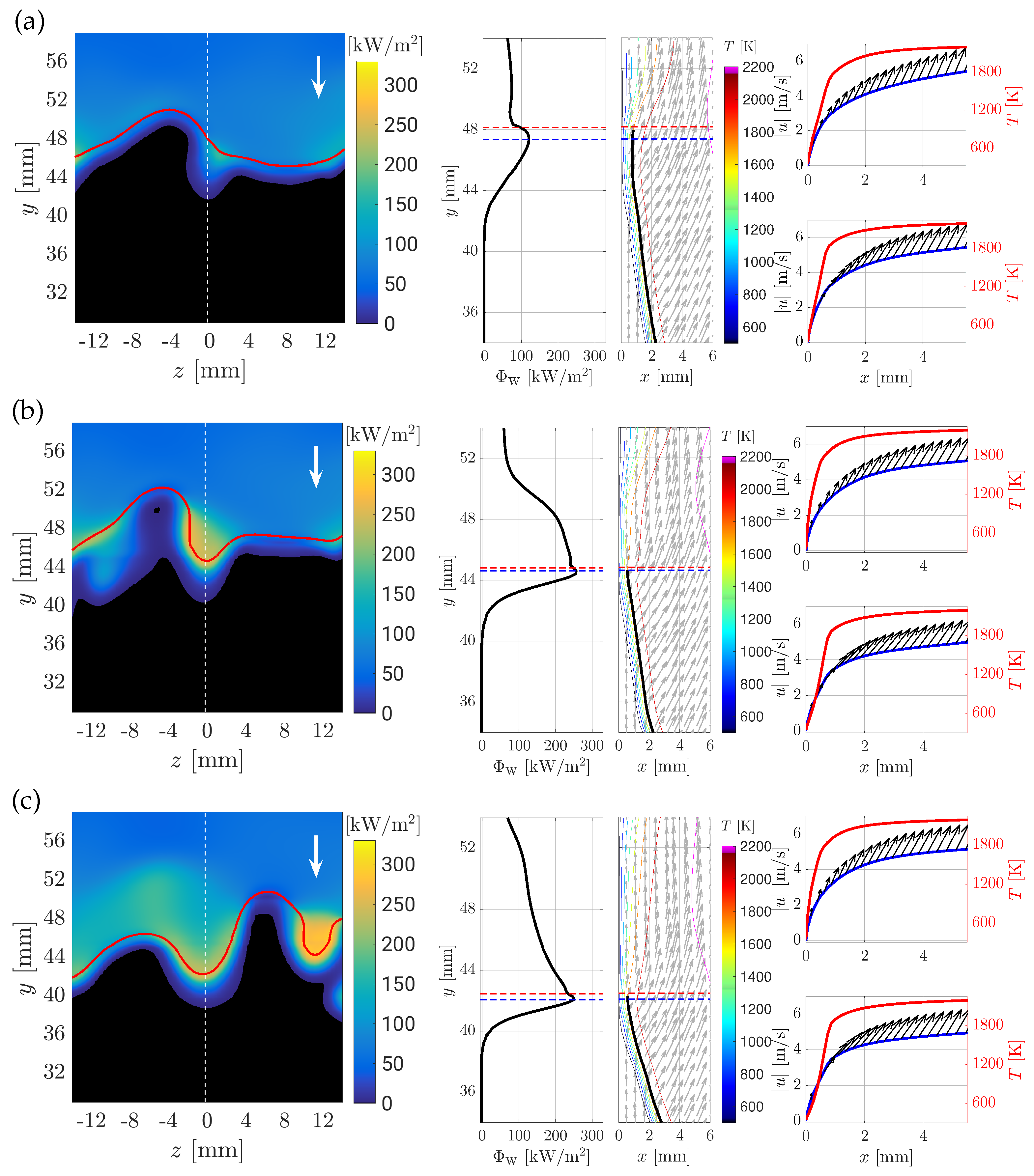
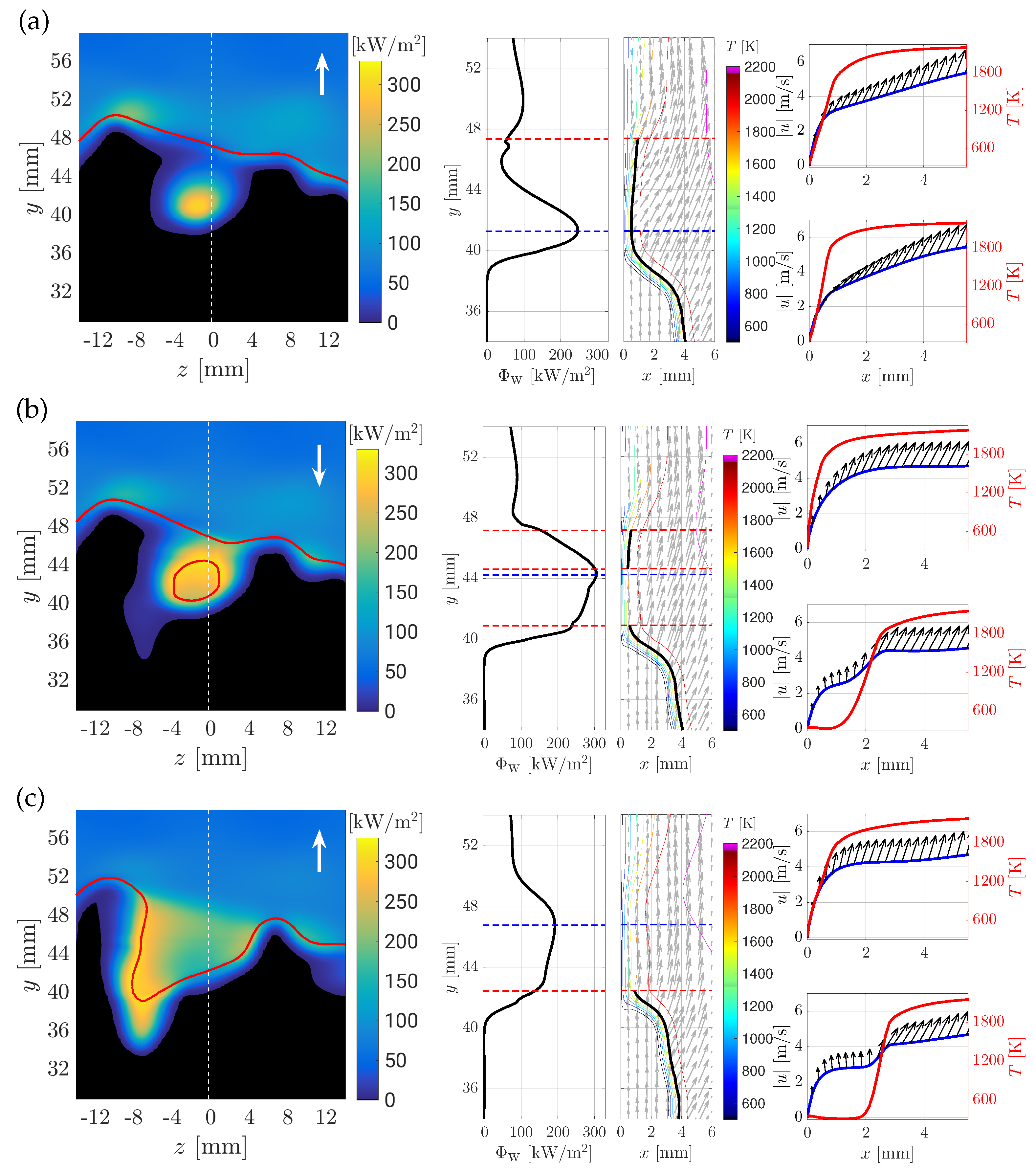
3.1. Description of the Quenching Point Movement

As pointed out by Heinrich et al. [17], the quenching positions, heat fluxes and wall angles are widely distributed. In this work, it will be shown that most of these statistics depend on the way the flame tip moves. The movement of the flame tip is tracked via the temporal quenching point position. A sequence from the center plane is shown in Figure 7, where the downstream and upstream movement are colored in green and red, respectively.

Clearly, this movement seems to be chaotic and is not equally distributed. In 71% of the events, the flame tip is moving in the downstream and in 27% in the upstream direction. Consequently, the averaged upstream velocity of the flame tip must be faster than its averaged downstream velocity. The remaining 2% are a jump-like upstream movement, with multiple quenching points along the wall. This leads to the following categorization:

(A)

A downstream movement,

(B)

A moderate upstream movement,

(C)

A jump-like upstream movement with multiple quenching points.

The following paragraphs together with the Figure 8, Figure 9 and Figure 10 describe the scenarios in more detail. The earliest time step is shown at the top and the latest on the bottom. The individual time steps are organized as follows (from the left to the right):

• two-dimensional contour plot of the wall heat flux together with the quenching line (red line), the position of the extracted profiles (z = 0 mm, white line) and the moving direction of the flame tip (white arrow)
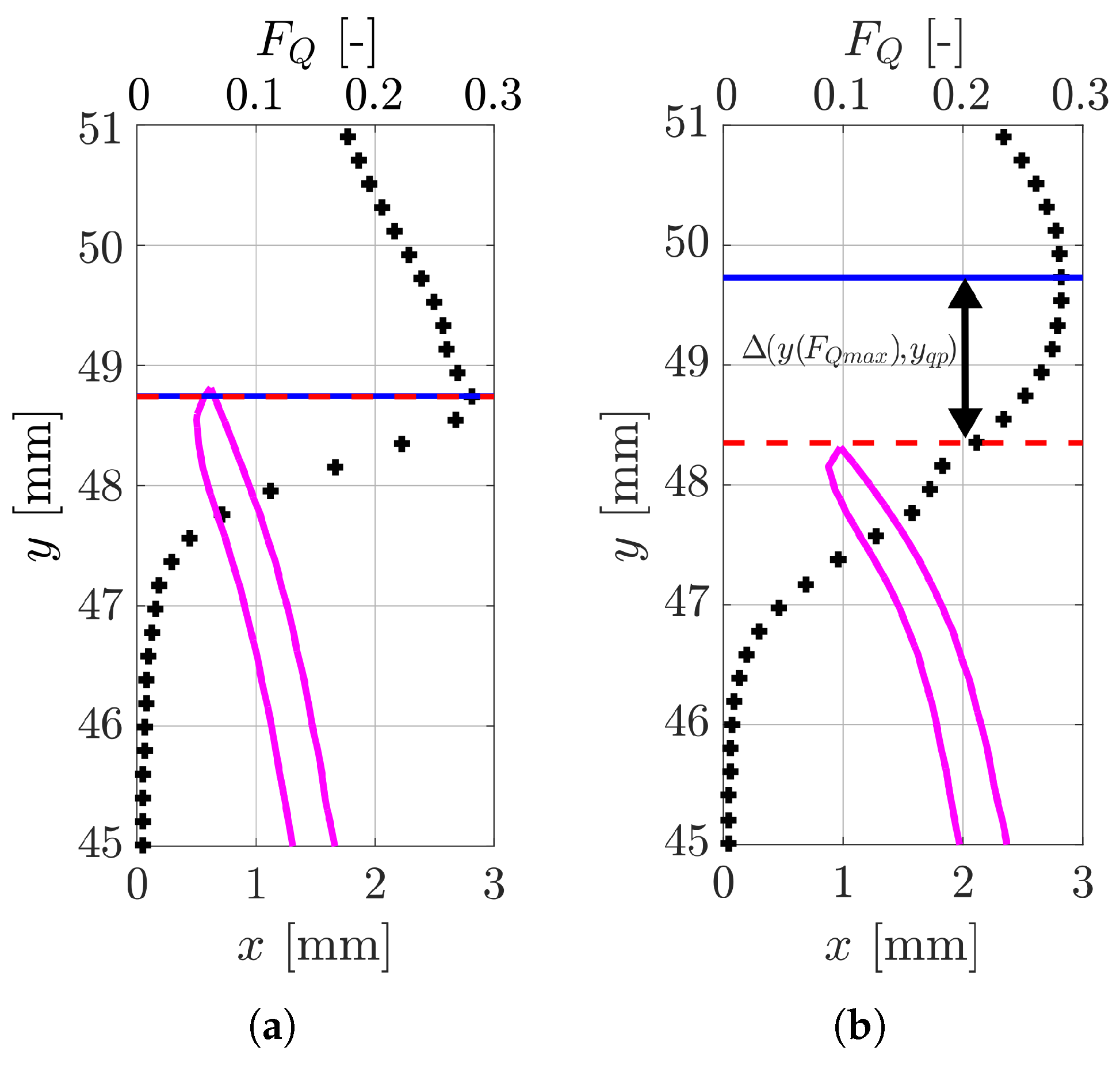
• ${\Phi }_{\mathrm{w}}$ along the wall at z = 0 mm, including the position of the maximum wall heat flux point $y\left({\Phi }_{\mathrm{w}}\right)$ (blue dashed line) and $y_{qp}$ (red dashed line),
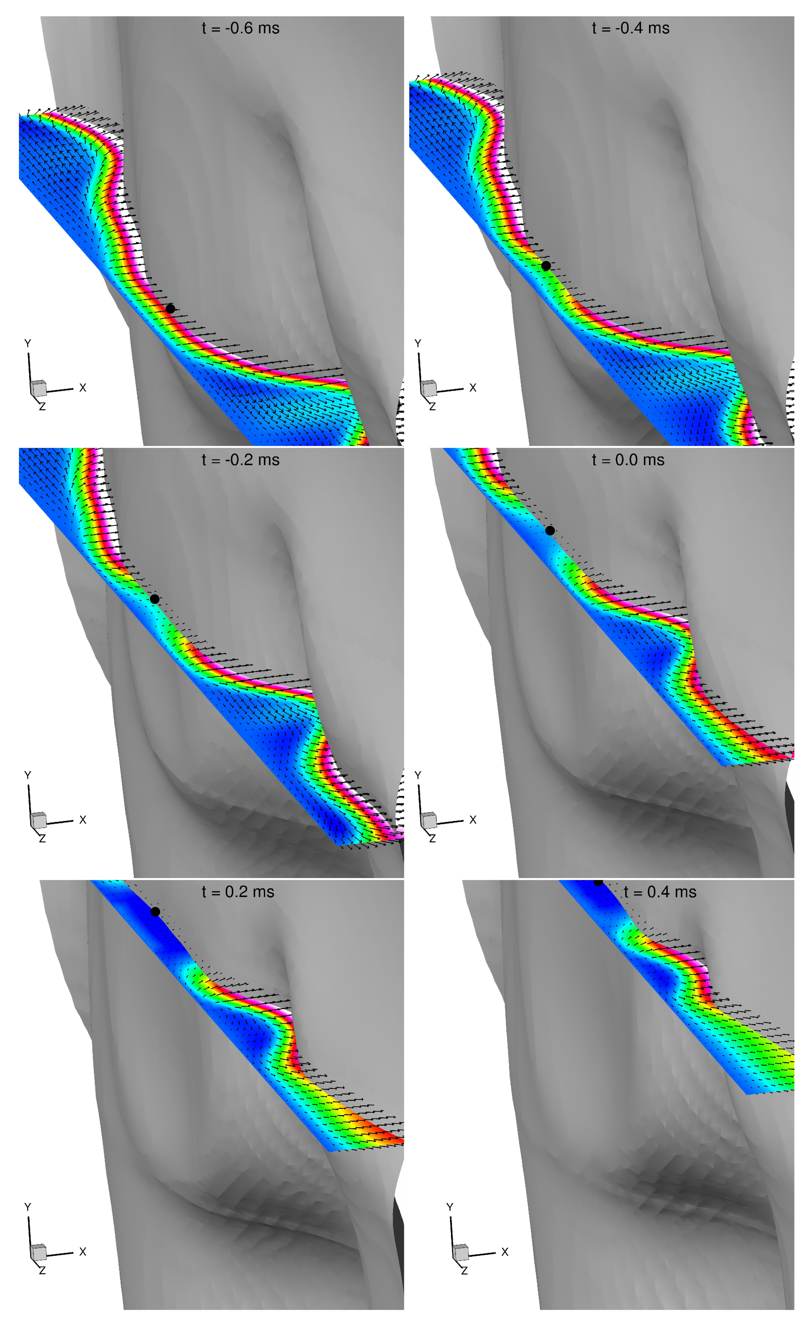
• a 2D slice (x-y-plane) with temperature isolines at z = 0 mm with the flame position (black line) overlaid with the velocity vectors and $y\left({\Phi }_{\mathrm{w}}\right)$ (blue dashed line) and $y_{qp}$ (red dashed line),
• the temperature field including the magnitude of the velocity and its vector for two positions at z = 0 mm (one at $y_{qp}$, one at $y_{qp}-4{\delta }_T$, where ${\delta }_T$ is the thermal thickness of the flame).

The explanations and statistics for scenarios are provided in the next sections.

(Scenario A)

The moderate downstream movement of the flame tip appears in nearly 71% of the cases, which makes it the most frequent event. How the flame and the wall heat flux are connected is explained in conjunction with Figure 8.

The quenching point $y_{qp}$ and the location of the maximum wall heat flux $F_{\mathrm{Q},max}$ move together in an axial direction, while the heat flux constantly decreases. As visible, $F_{\mathrm{Q},max}$ is downstream of the quenching point. The difference between both locations can be up to 12 thermal flame thicknesses. Within this movement and upstream of $y_{qp}$, mostly cold fresh gases flow parallel to the wall. This can be seen at the temperature field and at the extracted profiles. As visible on the right graphs, directly at the wall and 2 mm before the quenching point, the fluid is not heated by the flame. Compared to the laminar case, the heat fluxes are rather low and the quenching distances are large (${\Phi }_{\mathrm{w},\mathrm{l}}=200$ kW/m${}^2$, $P{e}_{\mathrm{q},\mathrm{l}}=7.3$).

(Scenario B)

The next scenario is depicted in Figure 9.

This moderate upstream movement with increasing maximum wall heat flux occurs in 27% of the events. The maximum heat fluxes and the quenching point are closely together, like in the laminar case, while the heat flux is mostly higher than in (scenario A) or than the laminar reference value ${\Phi }_{\mathrm{w},\mathrm{l}}=200$ kW/m${}^2$. Within this kind of movement, only high heat fluxes and low $P{e}_{\mathrm{q}}$ can be found. In contrast to (scenario A), no explicit temporal behavior of ${\Phi }_{\mathrm{w},\max }$ can be distinguished; within this movement, it can increase or decrease. Additionally, it can be seen from the temperature profiles on the bottom at right side of Figure 9 that the fluid upstream of the quenching position is heated by the flame.

(Scenario C)

The last scenario is found only in 2% of the cases. However, it cannot be neglected because only the strongest heat fluxes arise there. It is also an upstream movement like (scenario B), but it appears to look like a jump of the quenching point. Figure 10 will be used to explain the behavior. At the beginning (a), the flame front is nearly parallel to the wall and moves downstream like in (scenario A), but the wall heat flux upstream the quenching point increases at a large region. At the same moment, the flame gets weakened where the heat flux rises and the enthalpy near the wall decreases in the same area (not shown here). A widespread quenched region emerges (Figure 10b) and the heat flux reaches extreme values (up to $F_{\mathrm{Q},max}/F_{\mathrm{Q},max,l}=1.7$). In this moment, three quenching points occur in the center plane and the moving direction of the flame tip flips. Since the quenching point most upstream is always used as the reference point, it seems like it jumps upstream. As it can be seen in the left graph, in the next moment (c), both quenching areas will merge together and only one quenching point will remain. During this process, the occurring values of $F_{\mathrm{Q},max}$ are only the highest values. Afterwards, the flame tip moves downstream again with a lower heat flux, being the transition to (scenario A).

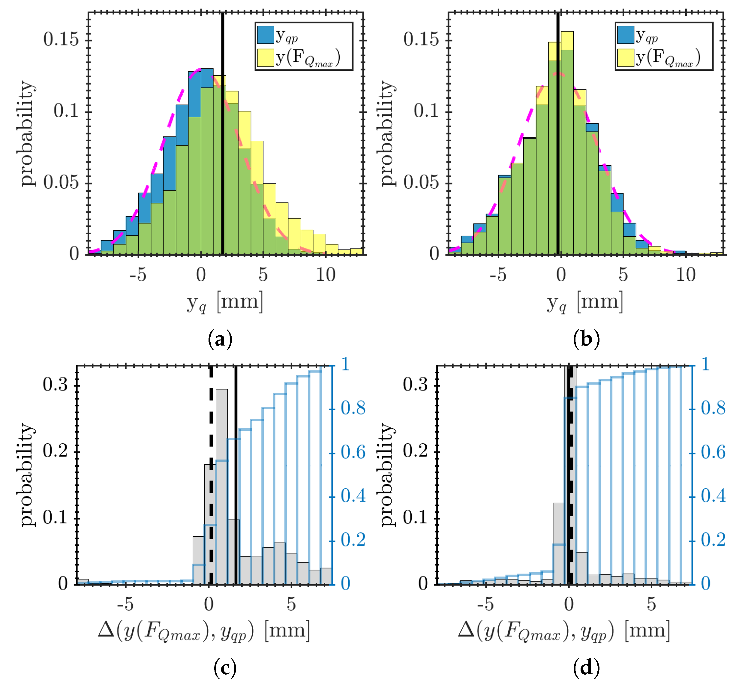
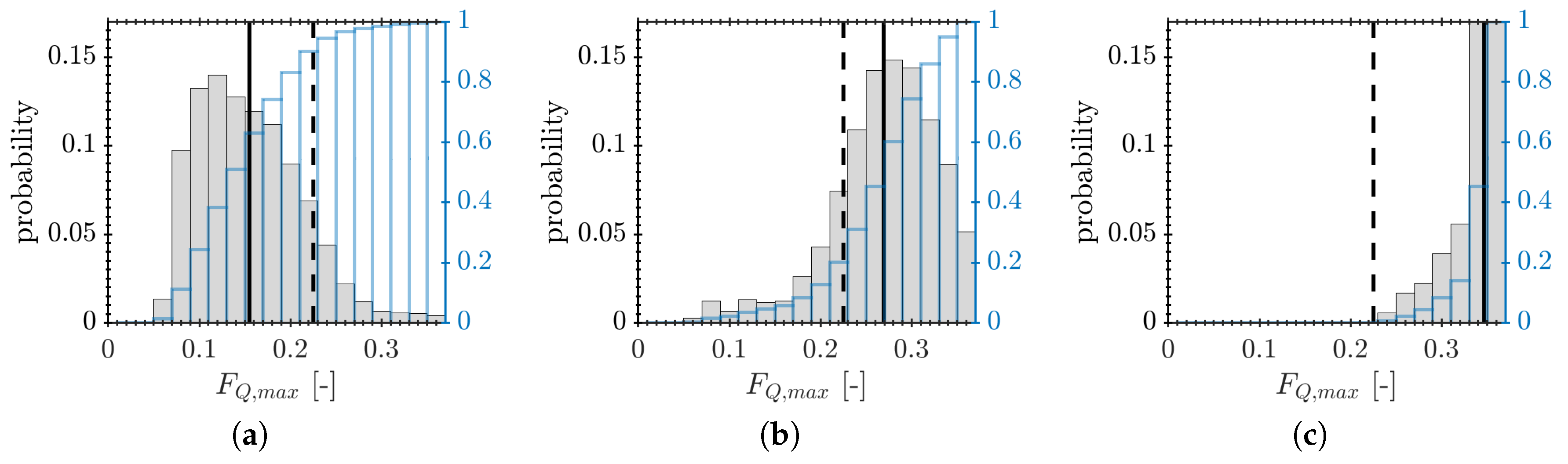
3.2. Statistics of the Axial Quenching Position and the Maximum Wall Heat Flux

As shown in Figure 11a, the locations of the maximum wall heat flux y($F_{\mathrm{Q},max}$) (blue solid line) and the quenching point $y_{qp}$ (red dashed line) are at the same position in a laminar SWQ flame. The black crosses correspond to the dimensionless wall heat flux profile (top x-axis) and the magenta line displays the iso-line ${\dot{\omega }}_{C{O}_2}=60$ kg/(m${}^2$s), which envelops the flame front. These profiles are shown in Figure 11b for one instantaneous moment of the turbulent SWQ configuration. As already observed by Heinrich et al. [17], in a turbulent setup, $y_{qp}$ and $y(F_{\mathrm{Q},max}$) do not always coincide. This phenomenon is visualized with the black arrow in Figure 11b. The quantity $\Delta (y\left(F_{\mathrm{Q},max}\right),y_{qp})=y\left(F_{\mathrm{Q},max}\right)-y_{qp}$ expresses the distance between the axial locations. A positive distance implies that the maximum heat flux is farther downstream. $F_{\mathrm{Q},max}$ and $y_{qp}$ are spacial quantities that change during time.

First, the temporal distribution of $y\left(F_{\mathrm{Q},max}\right)$ and $y_{qp}$ are analyzed in Figure 12a,b.

For both moving directions, $y_{qp}$ is centered at zero and normal distributed (magenta dashed lines). However, the mean value of $y(F_{\mathrm{Q},max}$) is zero for the upstream movement with equal number of counts the positive and negative side but with larger positive range. In contrast to that, the downstream direction has a mean value around 2 mm and more events occur on the positive side. The moving direction does not affect $y_{qp}$, but $y(F_{\mathrm{Q},max}$) because it is shifted for the downstream movement, which could be seen in Figure 8 in the graphs in the middle. The same observation can be made by looking at Figure 12c,d, where $\Delta (y\left(F_{\mathrm{Q},max}\right),y_{qp})$ is shown for all movements. In the following, most of the figures include similar histograms. A solid black line represents the mean value of the shown data and the dashed black the laminar reference. A cumulative histogram in light blue is overlaid. As it can be seen, within the downstream movement, for more than 60% of all events, the maximum wall heat fluxes are farther downstream. As a result, the mean difference is 1.8 mm. Like expected from the opposite direction (Figure 12b) and also visible in Figure 12d, $\Delta (y\left(F_{\mathrm{Q},max}\right),y_{qp})$ is very small (80% are in the range $|\Delta (y\left(F_{\mathrm{Q},max}\right),y_{qp}\left)\right|\le 1$ mm). Only a few outliers occur. The jump-like movement was not considered here because it is a very fast process whereby the determination of the local detachment is error-prone. Figure 12 showed that the shift between $y_{qp}$ and $y(F_{\mathrm{Q},max}$) is not constant and is mainly caused by the downstream movement of the flame tip.

Figure 13 displays the probability distribution of the maximum dimensionless wall heat flux. All three scenarios show a different behavior. If the flame tip moves downstream, only low values appear: nearly 90% are lower than the laminar reference. On the contrary, in the upstream scenario, 80% are higher than the laminar value. Accordingly, the mean values for these two cases are 0.155 and 0.27, respectively. The jump-like movement is most extreme; here, in 99% of the events, $F_{\mathrm{Q},max}$ is higher than the laminar scenario; accordingly, mostly the highest observed values appear. The distribution of the mean value of $F_{\mathrm{Q},max}$ depends on the movement of the flame tip; this was also shown in the representative snapshots in Figure 8, Figure 9 and Figure 10.

Another quantity, which was not discussed before, is the dimensionless heat flux at the quenching point $F_{\mathrm{Q},\mathrm{q}}$. Since it has a similar qualitative behavior to $F_{\mathrm{Q},max}$, its distribution will not be shown here. The difference is that the values for $F_{\mathrm{Q},\mathrm{q}}$ are a bit lower and the maximum values only appear at the upstream and jump-like movement. At the upstream movement, nearly 70% of the events are higher than the laminar reference with a mean value of $F_{\mathrm{Q},\mathrm{q}}=0.255$. The opposite applies for the downstream direction, almost 95% are smaller, with a mean value of 0.12. Both distributions ($F_{\mathrm{Q},\mathrm{q}}$ and $F_{\mathrm{Q},max}$) showed that high heat fluxes appear mostly while the flame tip moves upstream and the lowest values if it moves downstream.

As known from the literature (e.g., [5,17]), there is a negative correlation between $P{e}_{\mathrm{q}}$ and $F_{\mathrm{Q},\mathrm{q}}$. The cross-correlation between $P{e}_{\mathrm{q}}$ and $F_{\mathrm{Q},\mathrm{q}}$ is very strong, the correlation coefficients are −0.87 and −0.97 for the downstream and the upstream movement, respectively. With this in mind, the distribution of $P{e}_{\mathrm{q}}$ Figure 14 is not unexpected.

For the downstream direction, almost 90% of the events are higher than the laminar reference and the mean value is about $P{e}_{\mathrm{q}}=12$. This means that the flame is much farther away from the wall. The smallest possible wall distances do not occur. In contrast to that, only small distances occur for the upstream movement and its mean value $P{e}_{\mathrm{q}}=7.5$ is slightly below the laminar case. $P{e}_{\mathrm{q}}$ has a narrow distribution centered around its mean value with over 50% of the events in its proximity. The distribution for the jump-like movement is qualitatively similar to the upstream direction and the mean value $P{e}_{\mathrm{q}}=7.5$ is slightly lower than the laminar value. Certainly, the most events occur around $P{e}_{\mathrm{q}}=6.5$.

3.3. Physical Mechanism Governing the FWTI

Figure 14 displayed an obvious dependency of $P{e}_{\mathrm{q}}$ from the moving direction and, with its help, the occurring wall heat fluxes can be explained, since the flame can get close to the wall and a strong temperature gradient occurs. The resulting heat fluxes are very high or the opposite can occur, the flame is far away and the heat fluxes are much smaller.

The behavior for the downstream and upstream distributions can be explained with the temperature field. For that reason, time averaged temperature fields with respect to the conditioned coordinate system ($x_{\mathrm{q}}$, $y_{\mathrm{q}}$) are shown in Figure 15b,c.

Figure 15a shows the laminar temperature field for comparing purpose. Compared to the laminar case, in the downstream movement, more cold unburnt fluid is enclosed between the flame and the wall, which pushes the flame farther away from the wall. The consequence of this was shown before, the resulting heat flux is smaller. While the flame tip moves in an upstream direction, the temperature field is very close to the laminar case as already shown in Figure 14b. In addition, the flame shapes are different, depending on the movement. In case of the downstream movement, the curvature is stronger.

For a laminar SWQ flame, ${\Phi }_{\mathrm{w}}$ is always smaller than in the corresponding HOQ flame [5], but, as shown before, in the turbulent case, the wall heat flux can clearly exceed the laminar reference values up to values of the HOQ case or even higher. Due to that, the turbulent case will be compared qualitatively and quantitatively with an HOQ flame. Furthermore, a one-dimensional HOQ flame is calculated with FGM for this purpose. It has the same mixture properties as the main flow of the SWQ configuration and the same wall temperature. The one-dimensional grid used has the same resolution as the wall normal direction of the 3D SWQ case. As seen before in Figure 13, the jump-like movement has only the highest $F_{\mathrm{Q},max}$ values. This can be explained by analyzing this movement in a different conditioned coordinate system. Therefore, the location of the maximum wall heat flux $F_{\mathrm{Q},max}$ defines the zero on the y-axis. Figure 16 displays the time averaged temperature fields for all jump-like movements and the laminar reference.

As it can be seen on the right side, for the jump-like movement, the flame is nearly parallel to the wall, like in an HOQ manner. In addition, the temperature field is much more compressed in the direction of the wall, which causes the high heat fluxes. For a one-dimensional HOQ flame, the velocities near the wall are nearly zero at the moment the flame quenches. The same can be seen for the jump-like scenario in Figure 17.

Compared to the laminar case, where the flame is clearly an SWQ flame, the wall normal velocities are much smaller. Due to that, the flame can burn much closer to the wall because the convection away from it is much weaker.

Since the turbulent SWQ flame front is transient and three-dimensional, a point of interest has to be tracked in time and space. How it is done will be explained with Figure 18, Figure 19 and Figure 20.

A section of the 3D laminar flame is shown in Figure 18. On the left side, the wall is depicted for orientation purpose. The figure includes a temperature iso-surface of $T=1750$ K and a slice of the wall normal velocity component at the height of the maximum wall heat flux at the center of the burner. On the right side, a close-up view of the same section without the wall is displayed and the monitored quenching point is marked (black dot). Additionally, the momentum vectors are projected onto the slice. As it can be seen, the momentum vectors are all aligned and are pointed perpendicular away from the wall. The fluid is accelerated away from the wall by the flame without any redirection. Due to this convection, the flame cannot get closer to the wall.

The temporal evolution of the tracked point in turbulent case is shown in Figure 19 and Figure 20, (black dots). It follows the path of a point on the flame front, which leads to the maximum wall heat flux at $t=0$ ms.

As visible in the first sub-figure (top, left), the flame front is shaped convexly towards the unburnt gases. In contrast to the laminar case, the momentum vectors, which are not in the proximity of the tracked point, are directed away from the point into positive and the negative z-direction. During this progress, the wall normal velocity decreases and the convex flame shape gets flattened. Due to the convection of the main flow in the axial direction, the tracked point moves upstream while it stays more or less at the same z-position (which does not look like it is due to the chosen angle of view). By following this point, the graphs in Figure 21 and Figure 22 were created.

The temporal evolution of the tracked point from the turbulent SWQ setup, an HOQ flame and the laminar reference case are shown in Figure 21. It displays from the left to the right: the wall heat flux, the normal velocity and the position of the flame.

The time point $t=0$ ms marks the moment with the highest wall heat flux. The position and the velocity of the flame front are extracted, where the temperature is equal to 1750 K. This location coincides with the position of the maximum source term of the flame and therefore it is associated with the center of the flame.

At first, the 1D HOQ case will be illustrated. At the beginning, the heat flux rises up to its maximum value (at $t=0$ ms), while the wall normal velocity is positive and starts to decrease. At the same time, the flame moves towards the wall. It can been seen that the velocity is nearly zero when the highest heat flux appears, which is higher than the laminar SWQ case (black asterisk). After that, the velocity drops under zero, it stays negative, and the heat flux decreases again. The relation of the velocity and the temperature for the SWQ cases and the HOQ flame at characteristic points in time are plotted in Figure 22.

This kind of representation decouples the dependency of the spacial coordinate. Before the flame interacts with the wall ($t=-1.4$ ms, solid red line), the flame has a linear dependency, as the temperature increases the velocities increases, too. Right before the flame quenches ($t=-0.2$ ms), the velocity over the whole flame is reduced. Like seen before in Figure 21, at the moment of quenching, the velocity is very small. The high heat fluxes appear because the velocities between the flame and the wall decreases if the flame reaches the wall (Figure 21b,c), due to the fact that the flame can closely approach the wall, which leads to high temperature gradients. As already mentioned and known from the literature, the laminar wall heat flux is lower and the quenching distance is greater, which can be seen in Figure 21a,c. Due to the higher wall normal velocity in the laminar case, the convection away from the wall is greater, which explains why this flame is farther away from the wall (Figure 21b). The $T-u_x$ plot (Figure 22) reveals that the velocity in the laminar case is much greater than zero over most of the flame. Finally, the behavior of the turbulent SWQ flame will be discussed. The temporal evolution of the heat flux, the wall normal velocity and the flame position are also shown in Figure 21. Qualitatively, the shapes are similar to the one-dimensional HOQ flame. Certainly, the increase of the wall heat flux and the decrease of the velocity start earlier in the turbulent case because this flame is closer to the wall. The behavior right before the quenching occurs ($t=-0.2$ ms) is different too because the turbulent SWQ flame moves much slower. Furthermore, the linear dependency of the velocity from the temperature vanishes much faster for the SWQ flame; in the moment before quenching, it is gone. As it can be seen, at the moment of quenching ($t=0$ ms), the velocity of the HOQ is nearly zero over the whole temperature range, while, for the SWQ flame, the velocity is very small in the range of $T=300$ K–$T=1750$ K. After quenching, both flames have the same behavior for the region between the wall and the center of the flame. The drop of the velocity is also visible in the 3D plots in Figure 19 and Figure 20. As observed in these figures, the fluid moves away from the tracked point and, as a result, the wall normal velocity gets lower than in the laminar case. During this process, the convex shaped flame front gets flattened. As a result, the turbulent flame behaves locally like an HOQ flame because the effects of the velocity are getting negligible. The maximum wall heat flux is ${\Phi }_{\mathrm{w},\max }=311$ kW/m${}^2$ and the minimal wall distance is $x_{\min }=0.475$ mm, which are very close to the HOQ flame (${\Phi }_{w,max,HOQ}=313$ kW/m${}^2$, $x_{\min ,\mathrm{HOQ}}=0.417$ mm). After the turbulent flame reached the maximum ${\Phi }_{\mathrm{w},\max }$ ($t>0$ ms), the profiles from Figure 21 are nearly the same again. However, a difference can be seen in the $T-u_x$ plot (Figure 22), for the region far away from the wall, the velocity of the turbulent flame is much greater because the fluid of the SWQ flame can accelerate again.

With the knowledge gained above, the identified regimes are very natural and somehow obvious, but the characterization raises the question if also a jump-like downstream movement could appear. Therefore, pockets of fresh gases must appear downstream of the flame front inside the burnt region. In our configuration, this seems to be very unlikely and was not observed, but it could be possible e.g., if large eddies transport fresh gases into the burnt region. Due to the flame topology, these events would not be connected with high heat fluxes because the fresh gases do not preheat fluid near the walls.

4. Conclusions

This work was conducted to gain insight into the flame–wall–turbulence interaction. The analysis utilized results obtained from the simulation of a well-suited SWQ configuration where the statistical data was confirmed to be in good agreement with measurements. Building upon this predicting capability, the availability of the highly resolved, three-dimensional transient field gave access to the physical processes like the heat flux evolution that significantly depart from the laminar operation. First, several processes were identified that show a distinct phenomenological behavior associated with the quenching point displacement. Specifically, the three archetypes being the downstream, upstream and jump-like movements were shown to operate on individual time-scales and heat flux evolutions. This physical understanding was then supplemented with statistical evaluations confirming its generality. For this, the conditionally averaged data showed that the average downstream movement of the quenching point yields significantly lower heat fluxes than the laminar SWQ flame and vice versa for the upstream movement. Significantly larger heat fluxes were observed when the quenching point jumped. The root causes for this were subsequently identified by considering the full interaction of the turbulent field, the flame and the wall. It revealed that the near-wall flame wrinkling by turbulent structures locally creates a departure from the SWQ towards the HOQ regime. This latter is known for conditions that enable the flame to approach the wall very rapidly causing a strong interaction with high heat fluxes. We showed that, by the curvature of the flame towards the wall, these conditions can even get surpassed by a flame-tangential divergence of the velocity field.

The identification of the mechanisms of FTWI was conducted based on simulations of a laboratory scale experimental SWQ burner. The configuration was chosen first, since its geometrical complexity is a reasonable compromise in between computational effort and practical relevance regarding the process of interest and, second, basic validation data are available. With respect to the generality of the results and their relevance for future combustor design, it should be mentioned that the main goal of this work was to show that simulations with the given approaches can handle such configurations and their results provide a sound basis for an understanding of the physical processes. Considering the phenomenological character of our analysis, it is certainly transferable for in terms of the fundamental FTWI mechanism. However, the parameter specific to a configuration will decide how they scale and accordingly quantitatively behave. In this regard, the Reynolds number is generally higher in real applications, intensifying the FTWI. Accordingly, the mechanism of regime alteration (SWQ-HOQ) will likewise be enhanced. Furthermore, for regimes of higher Karlovitz numbers, stretch might further modify the near wall flame structure, causing significantly different peaks of the heat release. Likewise, the specific fuel is of major importance e.g., with respect to the pollutants formed in the walls vicinity. Similarly, the wall treatment (e.g., effusion cooling) will have an influence. In this regard, we mentioned that the tabulation approach should be chosen with care depending on the quantities of interest.

References

- International Energy Agency (IEA). World Energy Outlook; IEA: Paris, France, 2017. [Google Scholar]
- BP. Statistical Review of World Energy; BP: London, UK, 2018. [Google Scholar]
- Lazik, W.W.; Doerr, T.; Bake, S.S.; vd Bank, R.R.; Rackwitz, L.L. Development of Lean-Burn Low-NOx Combustion Technology at Rolls-Royce Deutschland. In ASME Turbo Expo: Power for Land, Sea, and Air; Volume 3: Combustion, Fuels and Emissions, Parts A and B; American Society of Mechanical Engineers (ASME): New York, NY, USA, 2008; pp. 797–807. [Google Scholar] [CrossRef]
- Dreizler, A.; Böhm, B. Advanced laser diagnostics for an improved understanding of premixed flame–wall interactions. Proc. Combust. Inst. 2015, 35, 37–64. [Google Scholar] [CrossRef]
- Poinsot, T.; Veynante, D. Theoretical and Numerical Combustion, 3rd ed.; Thierry Poinsot and Denis Veynante; Institut de Mécanique des Fluides de Toulouse: Toulouse, France, 2012. [Google Scholar]
- Cheng, R.; Bill, R.; Robben, F. Experimental study of combustion in a turbulent boundary layer. Symp. (Int.) Combust. 1981, 18, 1021–1029. [Google Scholar] [CrossRef] [Green Version]
- Gruber, A.; Sankaran, R.; Hawkes, E.R.; Chen, J.H. Turbulent flame–wall interaction: A direct numerical simulation study. J. Fluid Mech. 2010, 658, 5–32. [Google Scholar] [CrossRef]
- Saffman, M. Parametric studies of a side wall quench layer. Combust. Flame 1984, 55, 141–159. [Google Scholar] [CrossRef]
- Lu, J.; Ezekoye, O.; Greif, R.; Sawyer, R. Unsteady heat transfer during side wall quenching of a laminar flame. Symp. (Int.) Combust. 1991, 23, 441–446. [Google Scholar] [CrossRef]
- Ezekoye, O.; Greif, R.; Sawyer, R. Increased surface temperature effects on wall heat transfer during unsteady flame quenching. Symp. (Int.) Combust. 1992, 24, 1465–1472. [Google Scholar] [CrossRef]
- Boust, B.; Sotton, J.; Labuda, S.; Bellenoue, M. A thermal formulation for single-wall quenching of transient laminar flames. Combust. Flame 2007, 149, 286–294. [Google Scholar] [CrossRef]
- Alshaalan, T.M.; Rutland, C.J. Turbulence, scalar transport, and reaction rates in flame–wall interaction. Symp. (Int.) Combust. 1998, 27, 793–799. [Google Scholar] [CrossRef]
- Alshaalan, T.M.; Rutland, C.J. Wall heat flux in turbulent premixed reacting flow. Combust. Sci. Technol. 2002, 174, 135–165. [Google Scholar] [CrossRef]
- Jainski, C.; Rißmann, M.; Böhm, B.; Dreizler, A. Experimental investigation of flame surface density and mean reaction rate during flame–wall interaction. Proc. Combust. Inst. 2016, 36, 1827–1834. [Google Scholar] [CrossRef]
- Jainski, C.; Rißmann, M.; Böhm, B.; Janicka, J.; Dreizler, A. Sidewall quenching of atmospheric laminar premixed flames studied by laser-based diagnostics. Combust. Flame 2017, 183, 271–282. [Google Scholar] [CrossRef]
- Heinrich, A.; Ganter, S.; Kuenne, G.; Jainski, C.; Dreizler, A.; Janicka, J. 3D Numerical Simulation of a Laminar Experimental SWQ Burner with Tabulated Chemistry. Flow Turbul. Combust. 2017, 100, 535–559. [Google Scholar] [CrossRef]
- Heinrich, A.; Ries, F.; Kuenne, G.; Ganter, S.; Hasse, C.; Sadiki, A.; Janicka, J. Large Eddy Simulation with tabulated chemistry of an experimental sidewall quenching burner. Int. J. Heat Fluid Flow 2018, 71, 95–110. [Google Scholar] [CrossRef]
- Lehnhäuser, T.; Schäfer, M. Improved linear interpolation practice for finite-volume schemes on complex grids. Int. J. Numer. Methods Fluids 2002, 38, 625–645. [Google Scholar] [CrossRef]
- Smagorinsky, J. General Circulation Experiments with the Primitive Equations, 1. the basic experiment. Mon. Weather Rev. 1963, 91, 99–164. [Google Scholar] [CrossRef]
- Germano, M.; Piomelli, U.; Moin, P.; Cabot, W.H. A dynamic subgrid-scale eddy viscosity model. Phys. Fluids A Fluid Dyn. 1991, 3, 1760–1765. [Google Scholar] [CrossRef]
- Lilly, D.K. A proposed modification of the Germano subgrid-scale closure method. Phys. Fluids A Fluid Dyn. 1992, 4, 633–635. [Google Scholar] [CrossRef]
- Zhou, G.; Davidson, L.; Olsson, E. Transonic inviscid/turbulent airfoil flow simulations using a pressure based method with high order schemes. In Proceedings of the Fourteenth International Conference on Numerical Methods in Fluid Dynamics, Bangalore, India, 11–15 July 1994; Deshpande, S.M., Desai, S.S., Narasimha, R., Eds.; Springer: Berlin/Heidelberg, Germany, 1995; pp. 372–378. [Google Scholar]
- Van Oijen, J.A.; de Goey, L.P.H. Modelling of Premixed Laminar Flames using Flamelet-Generated Manifolds. Combust. Sci. Technol. 2000, 161, 113–137. [Google Scholar] [CrossRef] [Green Version]
- Smith, G.P.; Golden, D.M.; Frenklach, M.; Moriarty, N.W.; Eiteneer, B.; Goldenberg, M.; Bowman, C.T.; Hanson, R.K.; Song, S.; Gardiner, W.C., Jr.; et al. GRI-Mech 3.0, 1999. Available online: http://combustion.berkeley.edu/gri-mech/ (accessed on 1 September 2018).
- Chem1D. A One-Dimensional Laminar Flame Code, Developed at Eindhoven University of Technology. Available online: https://www.tue.nl/en/university/departments/mechanical-engineering/research/research-groups/multiphase-and-reactive-flows/our-expertise/chem1d/ (accessed on 1 September 2018).
- Van Oijen, J.A.; Lammers, F.A.; de Goey, L.P.H. Modeling of complex premixed burner systems by using flamelet-generated manifolds. Combust. Flame 2001, 127, 2124–2134. [Google Scholar] [CrossRef]
- Ketelheun, A.; Kuenne, G.; Janicka, J. Heat Transfer Modeling in the Context of Large Eddy Simulation of Premixed Combustion with Tabulated Chemistry. Flow Turbul. Combust. 2013, 91, 867–893. [Google Scholar] [CrossRef]
- Kuenne, G.; Euler, M.; Ketelheun, A.; Avdić, A.; Dreizler, A.; Janicka, J. A Numerical Study of the Flame Stabilization Mechanism Being Determined by Chemical Reaction Rates Submitted to Heat Transfer Processes. Zeitschrift für Physikalische Chemie 2014, 229, 643–662. [Google Scholar] [CrossRef]
- Avdić, A.; Kuenne, G.; Janicka, J. Flow Physics of a Bluff-Body Swirl Stabilized Flame and their Prediction by Means of a Joint Eulerian Stochastic Field and Tabulated Chemistry Approach. Flow Turbul. Combust. 2016, 97, 1185–1210. [Google Scholar] [CrossRef]
- Avdić, A.; Kuenne, G.; di Mare, F.; Janicka, J. LES combustion modeling using the Eulerian stochastic field method coupled with tabulated chemistry. Combust. Flame 2017, 175, 201–219. [Google Scholar] [CrossRef]
- Meier, T.; Kuenne, G.; Ketelheun, A.; Janicka, J. Numerische Abbildung von Verbrennungsprozessen mit Hilfe detaillierter und tabellierter Chemie. In VDI Berichte; Number 2162; VDI Verlag GmbH: Duisburg, Germany, 2013; pp. 643–652. [Google Scholar]
- Ganter, S.; Heinrich, A.; Meier, T.; Kuenne, G.; Jainski, C.; Rißmann, M.C.; Dreizler, A.; Janicka, J. Numerical analysis of laminar methane–air side-wall-quenching. Combust. Flame 2017, 186, 299–310. [Google Scholar] [CrossRef]
- Ganter, S.; Straßacker, C.; Kuenne, G.; Meier, T.; Heinrich, A.; Maas, U.; Janicka, J. Laminar near-wall combustion: Analysis of tabulated chemistry simulations by means of detailed kinetics. Int. J. Heat Fluid Flow 2018, 70, 259–270. [Google Scholar] [CrossRef]
- Williams, F.A. Combustion Theory: The Fundamental Theory of Chemically Reacting Flow Systems; Addison/Wesley Pub. Co.: Boston, MA, USA, 1985; p. 680. [Google Scholar]
- Colin, O.; Ducros, F.; Veynante, D.; Poinsot, T. A thickened flame model for large eddy simulations of turbulent premixed combustion. Phys. Fluids 2000, 12, 1843–1863. [Google Scholar] [CrossRef]
- Butler, T.; O’Rourke, P. A numerical method for two dimensional unsteady reacting flows. Symp. (Int.) Combust. 1977, 16, 1503–1515. [Google Scholar] [CrossRef]
- Durand, L.; Polifke, W. Implementation of the Thickened Flame Model for Large Eddy Simulation of Turbulent Premixed Combustion in a Commercial Solver. In ASME Turbo Expo: Power for Land, Sea, and Air; American Society of Mechanical Engineers (ASME): New York, NY, USA, 2007; Volume 2, pp. 869–878. [Google Scholar] [CrossRef]
- Kuenne, G.; Ketelheun, A.; Janicka, J. LES modeling of premixed combustion using a thickened flame approach coupled with FGM tabulated chemistry. Combust. Flame 2011, 158, 1750–1767. [Google Scholar] [CrossRef]
- Charlette, F.; Meneveau, C.; Veynante, D. A power-law flame wrinkling model for LES of premixed turbulent combustion Part I: Non-dynamic formulation and initial tests. Combust. Flame 2002, 131, 159–180. [Google Scholar] [CrossRef]
- Peters, N. Laminar flamelet concepts in turbulent combustion. Symp. (Int.) Combust. 1986, 21, 1231–1250. [Google Scholar] [CrossRef]
- Van Oijen, J.; Bastiaans, R.; de Goey, L. Low-dimensional manifolds in direct numerical simulations of premixed turbulent flames. Proc. Combust. Inst. 2007, 31, 1377–1384. [Google Scholar] [CrossRef]
- Van Oijen, J.; Groot, G.; Bastiaans, R.; de Goey, L. A flamelet analysis of the burning velocity of premixed turbulent expanding flames. Proc. Combust. Inst. 2005, 30, 657–664. [Google Scholar] [CrossRef]