Application of Machine Learning and Artificial Intelligence in Proxy Modeling for Fluid Flow in Porous Media

Abstract

Reservoir simulation models are the major tools for studying fluid flow behavior in hydrocarbon reservoirs. These models are constructed based on geological models, which are developed by integrating data from geology, geophysics, and petro-physics. As the complexity of a reservoir simulation model increases, so does the computation time. Therefore, to perform any comprehensive study which involves thousands of simulation runs, a very long period of time is required. Several efforts have been made to develop proxy models that can be used as a substitute for complex reservoir simulation models. These proxy models aim at generating the outputs of the numerical fluid flow models in a very short period of time. This research is focused on developing a proxy fluid flow model using artificial intelligence and machine learning techniques. In this work, the proxy model is developed for a real case CO₂ sequestration project in which the objective is to evaluate the dynamic reservoir parameters (pressure, saturation, and CO₂ mole fraction) under various CO₂ injection scenarios. The data-driven model that is developed is able to generate pressure, saturation, and CO₂ mole fraction throughout the reservoir with significantly less computational effort and considerably shorter period of time compared to the numerical reservoir simulation model.

1. Introduction

Developing a reservoir simulation model and conducting it for thousands of different scenarios ultimately provides us with a solution space which can be used for extensive uncertainty analysis. However, this technique essentially will be impractical for a geologically complex reservoir simulation model with millions of grid blocks, even if it requires only few hours for a single run to be accomplished. Although applying new technologies, such as cloud computing, can accelerate the process of running huge reservoir simulation models, it has its own complications; first of all these technologies are expensive and secondly, it would not be fast enough for a decision-making process. Encountering such a problem motivates the quest to find an alternative approach.

For the problem stated above, proxy models can be developed to approximate the solution of a complex reservoir simulation model. Although there is no proxy model that can generate exactly the same output as the original model, they can be significantly beneficial in approximating the desired outputs.

1.1. Proxy Modeling

Numerous efforts have been made to develop proxy models which can be used as a substitute for a complex reservoir simulation model. The proxy models, which have been developed in petroleum engineering, can generally be categorized into four different groups based on their development approach. These four groups are: statistics-based approach, reduced physics approach, reduced order modeling approach, and artificial intelligence (AI)-based techniques.

The statistical methods, such as response surfaces, try to generate a function that can capture the input–output relationship of the parameters involved. The number of inputs that can be used to develop the proxy model is limited to the uncertain parameters of the system. Even with this limited number of inputs, due to the statistical nature, this approach requires hundreds of simulation runs to properly cover the input–output space. In general, the more complex the mathematical function the more computational effort is required to obtain a proper function which can accurately describe the system behavior. In petroleum engineering, this technique has been applied in several types of studies such as history matching [1], upscaling geological models [2], field development planning [3], optimization [4], and many other studies. However, the most common area where this methodology has been applied is in uncertainty analysis of a particular process such as oil production [5,6] and CO₂ sequestration [7]. Other regression methods such as Gaussian process regression (GP) can also be applied to develop a response surface. This method was used by Zhang et al. to develop a proxy model for risk assessment of a geological CO₂ sequestration in a brine reservoir [8].

In proxy models based on reduced physics, the physics of the process is simplified by applying several assumptions. This approach is claimed to be more accurate due to the fact that the physics of the phenomenon is taken into account. However, it should be noted that the formulations which are used in petroleum engineering, and particularly those related to the fluid flow in porous media, are developed based on several simplifying assumptions and, therefore, they are already an estimation of what is actually happening in reality. As a result, the proxy models that are developed based on even further simplification of theses formulas barely represent the actual physics of the process, which significantly limits their application. In reservoir engineering, the reduced physics proxy modeling technique has most commonly been used in modeling thermal recovery processes such as SAGD (steam-assisted gravity drainage) and Vapex (vapor extraction), and also shale gas production. Using this approach, several proxies have been developed based on analytical formulations for modeling SAGD processes. Azad et al. used an analytical physics-based proxy model and the extended Kalman filter method for the purpose of reservoir characterization [9]. Vanegas et al. [10] developed a proxy model based on Butler’s formulation [11] for predicting oil flow rate, cumulative oil production, and cumulative steam injection under some uncertain parameters of porosity, horizontal permeability, vertical permeability, oil saturation, and rock type (shale or sand).

The reduced order modeling approach is used to reduce the computational effort of solving the system of non-linear equations pertaining to the fluid flow in porous media. This method is based on projecting the high-dimensional system matrix into a lower-dimension matrix through which the system of equations can be solved faster. Some of the techniques in this category are able to decrease the run time for a numerical reservoir model by several orders of magnitude. However, this procedure still needs to be performed on the full reservoir, and therefore it would not be as efficient when it is applied to a reservoir with a large number of grid blocks (over ${10}^6$). That is due to fact that in this approach, generating a low order model requires generating a system of partial differential equations for a large number of grid blocks. There is no doubt that in order to achieve a certain amount of accuracy, the order reduction cannot exceed a certain amount and, therefore, in practice, the reduced order model development for such a large number of grids becomes inefficient. Reduced order modeling has been applied in different areas for several purposes of simulation, classification, visualization, and compression of high-dimensional data. The application of this methodology in subsurface fluid flow modeling is relatively new, and is mostly based on Krylov subspace, balanced truncation, and proper orthogonal decomposition (POD) techniques. All of these approaches use projection methods to transform the high-dimensional state space of the original model into a low-dimensional subspace [12]. Proper orthogonal decomposition is probably the most commonly used method for the reduced order modeling of non-linear systems.

The reduced order models are beneficial in several types of problems such as optimization and uncertainty analysis where a large number of high order models are required to be performed. In reservoir engineering, POD has been vastly used as an approach to develop fast-running proxy models for a variety of numerical reservoir simulation models. However, many researchers have modified POD methodology in an attempt to enhance the results or the efficiency of POD through integrating some other techniques. For example, Cardoso et al. [13] have used a clustering technique to optimize the snapshots for the eigen-decomposition problem and missing point estimation (MPE) procedure to reduce the dimension of the POD basis vectors. Other techniques include the application of POD-TPWL (trajectory piecewise linearization) and POD-DEIM (discrete empirical interpolation method) which are elaborated further in this chapter.

Finally, proxy models can be constructed using machine learning and artificial intelligence techniques. Artificial intelligence and in particular artificial neural networks (ANN) have proven to be powerful data processing tools which have been applied to a wide variety of problems in different areas such as medical, engineering, financial, business, etc. An artificial neural network is a virtual intelligent technique which is an efficient tool for detecting and approximating the highly non-linear relationship between inputs and outputs of a system. During the last three decades this technique has been employed in petroleum engineering in different areas as an efficient tool to predict reservoir characteristics such as porosity and permeability, synthetic log generation, well production performance, etc.

The AI-based modeling approach can be viewed as finding the complex relationships between the input–output parameters involved in fluid flow simulation. This technique is the most flexible approach, which can be used for variety of problems regarding fluid flow in porous media such as uncertainty analysis, optimization, and history matching. This study is focused on using machine learning algorithms to develop a proxy model for numerical fluid flow model in porous media.

1.2. Application of Neural Networks in Fluid Flow Modeling

In the past three decades, neural networks have become of interest to petroleum engineers and geoscientists. On the subject of fluid flow in porous media, the supervised training algorithms and specifically backpropagation algorithm, are commonly used. In this method both the inputs and outputs are presented to the network and the learning process takes place based on error feedback to the network.

Artificial neural networks have been used for a variety of problems in petroleum engineering. The earlier applications of this method are well test interpretation [14], prediction of formation permeability [15,16], prediction of formation damage due to injection into low-permeability reservoirs [17] and reservoir characterization [18].

Later, applications of neural networks in several areas of petroleum engineering became more common. Gorucu et al. applied this methodology to construct a tool which was named a “Neurosimulation Tool”, with the objective of predicting the performance of a CO₂ sequestration process for enhanced coalbed methane [19]. Alajmi et al. developed a pressure transient analysis tool which was able to predict the desired unknown properties of a double-porosity reservoir system such as permeability of the matrix, porosity of the matrix, and fractures by training a neural network. In the training process they used the known properties of the reservoir, fluid properties, and well parameters as the neural network input [20]. Shihao wang et al. applied a deep learning algorithm to develop a model to perform flash calculation for compositional simulation in an unconventional reservoir [21]. The trained neural network is able to predict the phases and concentration distribution in the system with very low computational cost and high accuracy. They used this result as the initial guess for the flash calculation module in the reservoir simulator. Flash calculation requires very time-consuming numerical calculations which encounter stability problems in some cases, and therefore implementing deep learning algorithm in flash calculation module resulted in much faster results with improved stability.

In another study performed by Mohaghegh et al. a well-based surrogate reservoir model (SRM) was developed for a giant oil field in the Middle East in order to identify the wells that are prime candidates for rate relaxation with the objective of higher oil production. The field production after more than two years confirmed the results predicted by the SRM surrogate reservoir model developed which demonstrated the capability of the reservoir models developed based on neural network in real field operation [22].

Shahkarami et al. have used the AI-based approach to develop an assisted history matching technique for a synthetic oil field with 24 production wells and 30 years of production. The history matching process in this study is based on three uncertain parameters of the reservoir which are porosity, permeability and thickness. The results of this study showed that neural networks can be used as a fast and efficient tool for assisted history matching process [23].

Klie and Florez applied a new approach to develop a data-driven model for fractured shale reservoirs [24]. In this work, the data-driven model included dynamic mode decomposition (DMD) for modeling the pressure field. DMD is used for state estimation, forecasting and control based on reduced-order systems, as an alternative to POD. A long short-term memory (LSTM) network, which is a type of recurrent neural network (RNN), is trained to track gas production.

In general, according to the existing literature, artificial intelligence techniques have been mostly used to develop proxy models, which aim at computing wellbore related parameters such as production/injection rather than dynamic parameters of the reservoir such as pressure and gas saturation. The well-based models are constructed for a variety of problems including well performance analysis, optimization, history matching, etc.

There are only a few studies that have been conducted using artificial neural networks for the purpose of flow modeling within the porous media. In a study performed by Klie [25], POD and DEIM methodology and radial basis function (RBF) networks were used to develop a proxy model with two objectives of production rate prediction, and also pressure and gas saturation distribution under uncertain permeability and varying injection rate. POD and DEIM were used as a tool to reduce the dimensionality of the matrices generated which are going to be used as inputs for the RBF network. Therefore, they need to go through all the complications of the POD methodology, before they can use the RBF network to develop the proxy model. This methodology has been applied on two reservoir models with maximum of 300 grid blocks. Applying such techniques when the number of grid blocks increases, dramatically increases the computational time and effort to build such proxy models, and therefore is not practical for more realistic numerical reservoir models in terms of size and complexity.

In the research performed by Chen et al. [26], a proxy model was developed for a 2D reservoir model with 900 grid blocks and a heterogeneous permeability distribution with constant porosity. They assumed that saturation is known and tried to predict the pressure at each grid block by using the simplified developed proxy model using artificial neural networks. In this work a very simplified formulation and reservoir model has been used which does not demonstrate the ability of the model to be applied for a more realistic case.

The existing studies on the application of artificial neural network for developing a grid-based SRM or proxy model have many limitations and deficiencies and, therefore, they cannot be used as a practical tool for a complex numerical reservoir simulation model. The current work uses a novel approach to develop a surrogate reservoir (proxy) model by using artificial neural networks. The capability of the developed model is demonstrated by applying the technique to a real case, 3D heterogeneous reservoir with 100,000 active grid blocks which is used for a CO₂ sequestration study.

2. Materials and Methods

The work flow which was followed to develop the fluid flow proxy model is presented in detail in the following sections.

2.1. Numerical Reservoir Model Development

2.1.1. Field Background

The understudy field is a depleted gas reservoir. This field was identified as a proper option for CO₂ sequestration since the site is well characterized due to its natural gas production history [27]. The target reservoir for injecting CO₂ is a sandstone reservoir approximately 110 ft thick and located 6561 ft underground with an area of about 500 acres. The reservoir is overlain by a caprock of mudstones. The structure is bound with three major sealing faults and two aquifers which are connected to the reservoir from south-east and west side. Two wells exist in this reservoir. The first well was a natural gas production well, producing from May 2002 to October 2003 that was converted to a monitoring well in 2007. The second well (CRC-1) is an injection well through which the CO₂ was injected underground. It was drilled in 2007 and is located approximately 980 ft away from the previously producing well. CO₂ injection through CRC-1 started in March 2008 [28].

In the next step a numerical reservoir simulation model is developed to simulate both the natural gas production phase, and the CO₂ injection phase. However, further studies in this work are only focused on the CO₂ injection process. The reservoir model is developed in CMG-GEM (compositional modeling module, Computer Modelling Group Ltd., Calgary, AB, Canada) using the available field data.

The structure of the reservoir is generated by making use of a contour map available from the geological information of the field. This model includes 100 × 100 grid blocks in the x–y direction and consists of 10 layers. The reservoir structure and well locations are depicted in Figure 1. The production well is completed in layers 5 and 6; however, the injection well is completed in five layers of the reservoir (layer 3 to layer 7).

Reservoir parameter distribution (porosity and permeability) is generated through a statistical method (Kriging) using the CRC-1 core and log data.

When injection takes place in the reservoir, hysteresis phenomenon plays a significant role on fluid flow behavior. In the early injection period, drainage is the dominant process; however, imbibition takes place when the CO₂ plume starts migrating. Hysteresis affects the CO₂ mobility as well as the gas water contact, and therefore is introduced to the model through the proper relative permeability curves.

Due to the existence of an active aquifer system, a fraction of the injected CO₂ is dissolved into the water phase and, therefore, in this model the CO₂ solubility in water is also taken into account.

2.1.2. History Matching

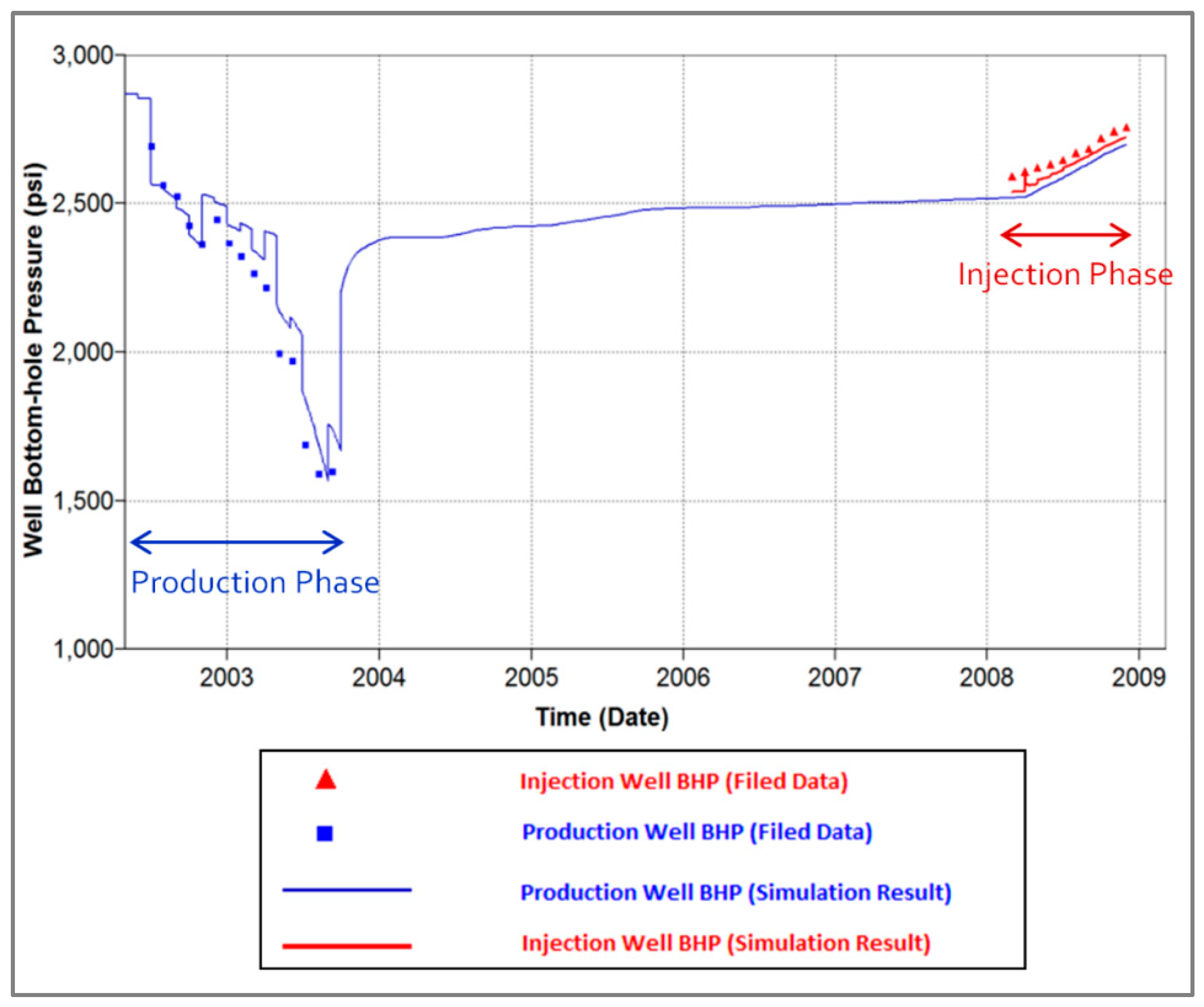
The developed reservoir model was history-matched based on the available field data both in the natural gas production phase and the CO₂ injection phase. During the history-matching process the monthly natural gas production rate for 18 months and the monthly CO₂ injection rate for 8 months are considered as the constraint in the model and the well bottom-hole pressure is matched for the production and injection wells by altering the reservoir parameters. The thickness of the reservoir layers was assumed to be a constant value equal to 11 feet. Therefore, during the history-matching process, the porosity and permeability of the reservoir are used as the major tuning parameters. Figure 2 shows the field data and the simulation results for bottom-hole pressure (BHP) of the production and injection wells after history matching.

The history matched model is used as a base model to generate the grid-based SRM for the injection interval when the model is executed for several injection scenarios.

2.2. Proxy Model Development

Surrogate reservoir modeling is an AI-based approach to construct a proxy model that can be used to generate the outputs of a complex numerical reservoir simulation model. In this context, SRM can be defined as a customized model comprised of a collection of neural networks which are trained, tested, and verified for a specific problem.

Once developed for a particular case, it can generate the outputs of the numerical reservoir simulation model when the inputs are altered within a specific range which the networks have been trained with.

For this work, SRM is developed to investigate the changes of dynamic parameters (pressure, gas saturation, and CO₂ mole fraction) throughout the reservoir under various injection scenarios. Figure 3 shows the general work flow to SRM development.

2.2.1. Simulation Scenario Design

As mentioned before, for the purpose of SRM development, only the injection phase is considered. For this study a constant injection interval of 24 months is used and five CO₂ injection scenarios are designed based on the amount of CO₂ injected into the reservoir. Assuming G as the total amount of CO₂ injected for the base case, in the four subsequent scenarios, 2G and 3G, 3.25G and 3.5G total CO₂ is injected into the reservoir in 24 months. The monthly injection rates for all the above scenarios is depicted in Figure 4.

2.2.2. Data Set Generation

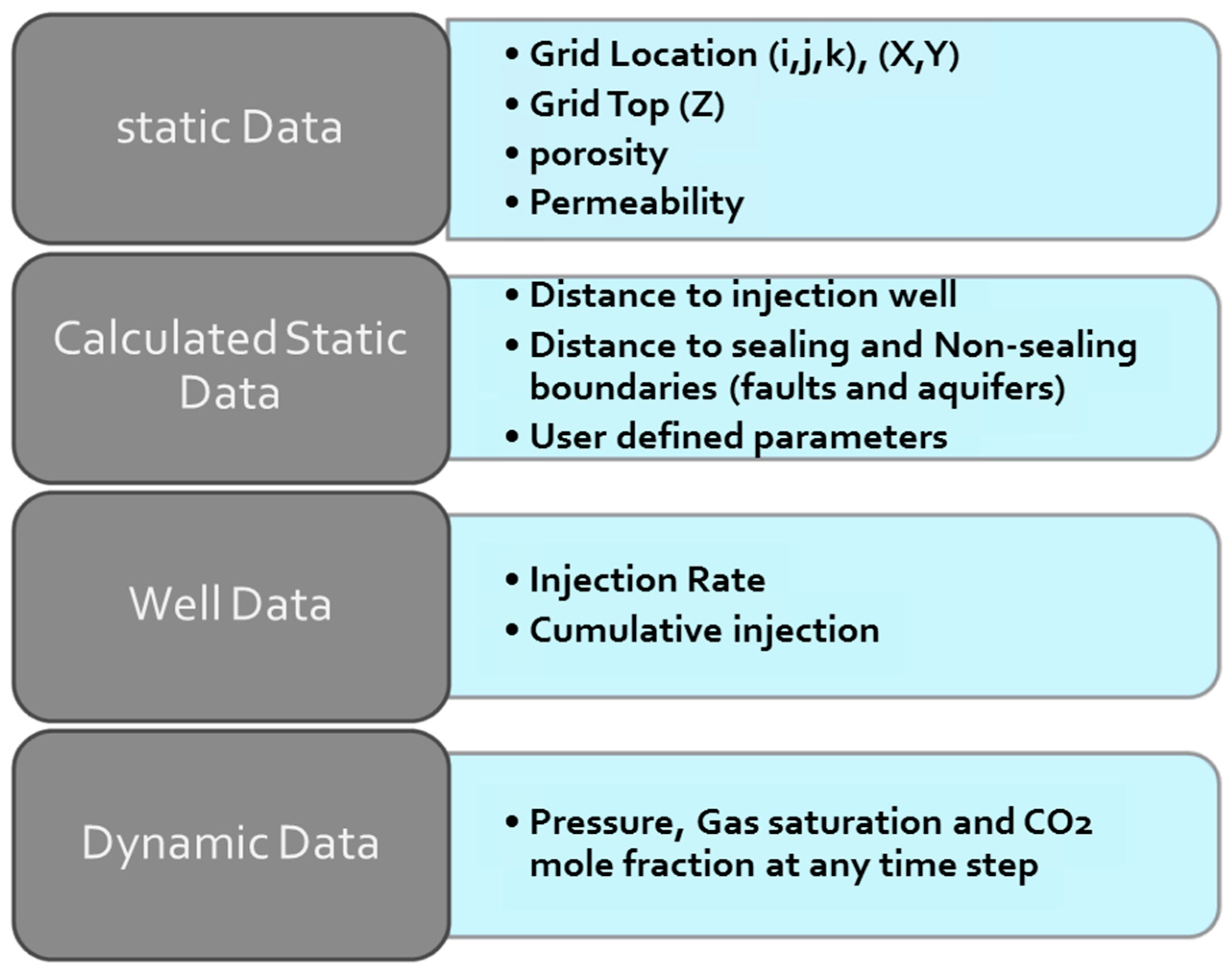
The five above injection scenarios are executed, and proper static and dynamic data are extracted at the grid block level from the numerical reservoir model. The dynamic parameters are collected at each month of injection for the entire injection interval. Subsequently, a comprehensive spatio-temporal data set is generated for all injection scenarios. A list of parameters included in the data set is presented in Figure 5.

In CO₂ injection and sequestration process, since CO₂ is migrating upward, CO₂ mole fraction, and as a result gas saturation at any location of the reservoir, depend on the reservoir characteristics (such as porosity and permeability) of not only the current layer, but also the lower and upper layers. The available pore volume and degree of tightness of several grid blocks in the vicinity of the main grid block affect CO₂ movement and gas saturation distribution. Therefore, in order to take into account the effect of this dependability, extra parameters are calculated and included in the data set (Figure 6). To obtain the value of Tier-1, Tier-2, and Tier-3, the average reservoir parameter is calculated over the grids which are included in the corresponding tier system. It should be mentioned that the number of grid blocks included at each tier system can be increased or decreased, based on the model resolution.

2.2.3. Data Sampling

Since the main dataset includes data from every single grid block of the reservoir for five different scenarios, the generated dataset is very high-dimensional and, therefore, very time consuming to be used for neural network training purposes. Therefore, data sampling is used to reduce the dimensionality of the dataset.

At each time step, data are sampled based on the amount of changes in dynamic parameters compared to the initial state of injection; meaning that the 10% of the data are more selected from the grid blocks with higher amount of changes in dynamic parameters. This approach is used to ensure that the sampled data are able to properly represent the changes that are happening in the reservoir due to CO₂ injection. Applying this methodology, 10% of the entire data at each time step is selected to be used for training the proxy model.

2.2.4. Proxy Flow Model Development

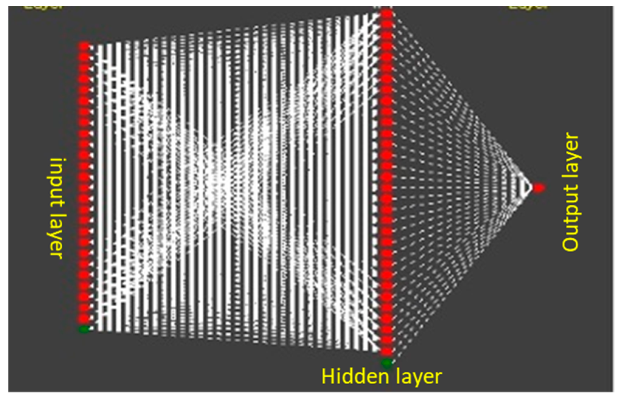
In general, neural network is considered as a class of non-linear parametric function, where the parameters are tuned during the neural network training. In this work, back propagation neural network is used to develop the proxy model. Neural network training will be performed once the network structure is determined. In the current study, a three-layer neural work (input layer, one hidden layer, and one output layer) is used. The general structure of the network is depicted in Figure 7. The number of neurons in the input layer is equal to the number of features used as input parameters. In the hidden layer, the number of neurons are chosen to be slightly higher than the number of inputs. The input features include the parameters listed in Figure 5, as well as the average porosity and permeability at three-tier systems, for all grid blocks of the reservoir. All the features in the generated dataset in Section 2.2.2 are normalized between −1 and 1.

At each monthly time step during the injection, three individual neural networks are trained for pressure, gas saturation, and CO₂ mole fraction. Therefore, there is one output for each network at each time step.

The neural network training process comprises several steps that lead to the determination of the involved network parameters. In the back propagation method, at each training epoch the calculated error is sent backward through the network and the weights are updated accordingly. Gradient descent method was used as an optimization algorithm to minimize the error. During the neural network training, some network hyper parameters such as momentum and learning rate are tuned to get a better accuracy.

The data set is randomly partitioned into three parts. For each of the neural networks 80% of the input data (out of the already sampled data) is used for training, 10% for validating, and 10% for testing.

During the training process, performance of the neural networks in predicting the output parameter is investigated by observing the cross plots of the neural network predicted values versus simulation output, and also changes of the R-squared value for the training, validation and test set. The error of the training set as well as the validation set is observed to make sure at each epoch these two errors are decreasing. The model training is stopped when two criteria are met. First, a satisfactory R-squared value is obtained, and second the validation set error is not decreasing any more. The latter prevents the overfitting problem where the training set error is still decreasing.

3. Results

3.1. Proxy Model and Numercial Model Output Comparison

As mentioned in the previous section, only 10% of the entire data was sampled and used to train the neural networks. In order to generate the dynamic reservoir parameters for the entire reservoir, the developed neural networks at each time step (each month of injection), are applied to all grid blocks of the reservoir.

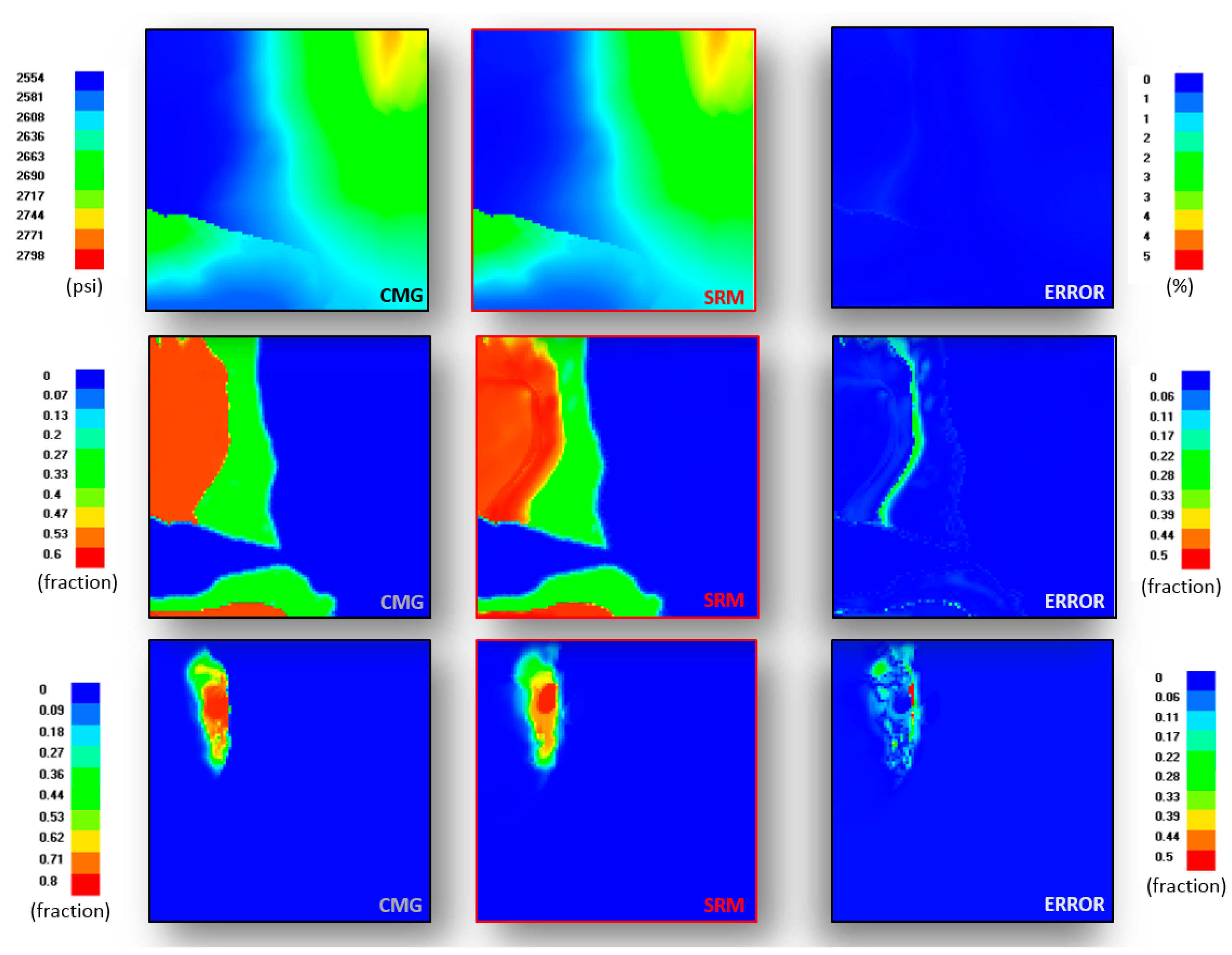
To evaluate the result of the trained proxy model in generating the outputs of the numerical reservoir model, the developed model is applied to a training dataset (scenario-2) and the distribution of dynamic parameters in the reservoir at each time step is compared. In Figure 8 and Figure 9, the distribution maps of the three parameters of pressure, gas saturation and CO₂ mole fraction at the first layer of the reservoir are presented for two time steps during the injection process (in the middle of the injection and at the end of the injection).

In order to verify the capability of the developed model to generalize, the model is applied on a blind case scenario which was not used in the training process. Therefore, a new injection schedule is defined and executed in the reservoir simulation model. The monthly gas injection schedule for the blind case scenario is depicted in Figure 10 with crossed lines.

Subsequently, the required data are extracted from this scenario and the developed proxy model is applied to generate the three output parameters throughout the reservoir over the entire injection interval. The results of the neural network predictions for the three dynamic parameters are presented in Figure 11 and Figure 12.

3.2. Proxy Model Error Evaluation

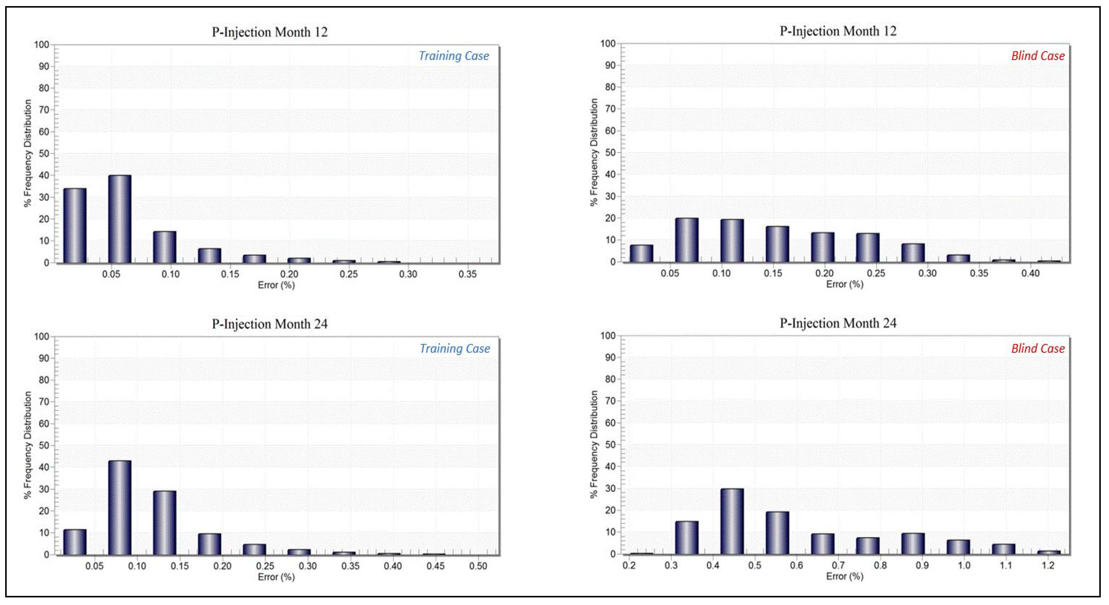
The 2D distribution maps, which were presented in the previous sections, visualize the proxy model result versus the CMG output for each layer of the reservoir. In this section, the frequency error plots are presented to demonstrate the frequency distribution of the error for all grid blocks of the reservoir. The error plots were generated for each parameter of pressure, gas saturation, and CO₂ mole fraction individually, when neural networks are applied to two different scenarios (the training case and the blind case). As an example, the results are presented at two time steps during the injection interval for both scenarios (Figure 13, Figure 14 and Figure 15).

Generally, the frequency of the grid blocks with higher amount of error increases when the neural networks are applied to the blind case as opposed to the training case, especially in the later time steps.

Also the results show that the pressure networks have the highest acuracy in predicting the pressure distribution since for this parameter the amount of error for the blind case scenario after 24 months of injection does not exceed 2%. The frequency error plot for gas saturation prediction for the same blind case after 24 months of injection shows that about 85% of the grid blocks have an error of less than 0.02. The prediction results for the same case for CO₂ mole fraction show that more than 95% of the grid blocks have an error of less than or equal to 0.05.

In general, pressure distribution generated by the proxy model is of very high accuracy (less than 3% of error) compared to gas saturation and CO₂ mole fraction. The reason lies in the fact that the reservoir has a relatively small volume with strong aquifer support and, therefore, the entire reservoir is pressurized as a result of CO₂ injection. Consequently, pressure does not have a clear front which needs to be specifically detected. This can be the reason why the changes in pressure can be captured effectively through the sampled data.

The output for gas saturation and CO₂ mole fraction shows higher error. The reason is that both of these two parameters have a sharp front and, therefore in order to be accurately detected, a sufficient amount of data is required to be introduced to the network particularly from the areas close to the edge of the plume. Although the sampling methodology is based on selecting the majority of the data from the area with maximum amount of change, it does not guarantee selection of all the data specifically from the edge of the CO₂ plume.

4. Discussion

Due to the limitation of the computational power available for this study, the neural network training was performed using only 10% of the data from the training scenarios; however, using a much higher percentage of the data set extracted from the training scenarios can improve the results of the neural network prediction. The more training data that is used, the better the fluid flow behavior can be captured during the training process.

In this work a single layer neural network algorithm was used to develop the proxy model; however, application of deep neural network is recommended, specifically if a large percentage of the reservoir grid blocks are used in the training phase.

5. Conclusions

The developed proxy model based on artificial intelligence and machine learning is capable of generating the results of a complex numerical simulation model at the grid block level with reasonable accuracy in a very short period of time with significantly less computational cost. It takes about 15 mines to execute one of the simulation runs used in this study, and it takes about 45 s to apply the developed neural networks for all monthly time steps. Therefore, we have speeded this up by about 20 times for this specific case. However, the more complex the reservoir model, the higher it is speeded up. That’s because when the reservoir model gets more complicated the run time to solve the partial differential equations would dramatically increase; however, the time and computational effort to develop and apply a neural network for such a complex system is not increasing accordingly. Therefore, the efficiency of the proxy model is much higher for more complex systems.

The AI-based proxy model is not limited by the choice of a predefined function and, therefore, it is very flexible. In all the proxy models developed through statistical approaches, the function that represents the system behavior is solely determined through the relationships between the uncertain parameters and the system outputs. However, in an AI-based approach any type of data which affect the output of the model or provides any information regarding the under study system can be included in model development. Therefore, the model is trained by providing information related to any component of the system, the relationship between these components, and the effect of each of them on system behavior.

An AI-based proxy model can be used to model a significantly non-linear system. The pattern recognition capability of neural networks enables the model to capture the interrelationship between multiple parameters of the system without encountering any instability problems.

The characteristic of the method used in this study allows us to make use of several types of data in order to teach the model the physics behind the fluid flow in porous media. Therefore, the constructed model is able to generate the outputs of the numerical simulation model when the inputs are changes within the training range.

References

- Slotte, P.A.; Smorgrav, E. Response Surface Methodology Approach for History Matching and Uncertainty Assessment of Reservoir Simulation Models. In Proceedings of the Europec/EAGE Conference and Exhibition, Rome, Italy, 9–12 June 2008. [Google Scholar]
- Narayanan, K.; White, C.D.; Lake, J.W.; Willis, B.J. Response Surface Methods for Upscaling Heterogeneous Geologic Models. In Proceedings of the SPE Reservoir Simulation Symposium, Houston, TX, USA, 14–17 February 1999. [Google Scholar]
- Carreras, P.E.; Turner, S.E.; Wilkinson, G.T. Tahiti: Development Strategy Assessment Using Design of Experiments and Response Surface Methods. In Proceedings of the SPE Western Regional, Anchorage, AK, USA, 26–27 May 2006. [Google Scholar]
- Purwar, S.; Jablonowski, C.J.; Nguyen, Q.P. A Method for Integrating Response Surfaces into Optimization Models with. In Proceedings of the SPE Hydrocarbon Economics and Evaluation Symposium, Dallas, TX, USA, 8–9 March 2010. [Google Scholar]
- Ahmed, S.J.; Recham, R.; Nozari, A.; Bughio, S.; Schulze-Riegert, R.; Ben Salem, R. Uncertainty Quantification Workflow for Mature Oil Fields: Combining Experimental Design Techniques and Different Response Surface Models. In Proceedings of the SPE Middle East Oil and Gas Show and Conference, Manama, Bahrain, 10–13 March 2013. [Google Scholar]
- Al Salhi, M.S.; Van Rijen, M.F.; Dijk, H.; Wei, L. Structured Uncertainty Assessment for Fahud Field through the Application of Experimental Design and Response Surface Methods. In Proceedings of the SPE Middle East Oil and Gas Show and Conference, Manama, Bahrain, 12–15 March 2005. [Google Scholar]
- Yeten, B.; Castellini, A.; Guyaguler, B.; Chen, W.H. A Comparison Study on Experimental Design and Response Surface Methodologies. In Proceedings of the SPE Reservoir Simulation Symposium, The Woodlands, TX, USA, 31 January–2 February 2005. [Google Scholar]
- Zhang, Y.; Pau, G. Reduced-Order Model Development for CO2 Storage in Brine Reservoirs; Technical Report Series; Earth Sciences Division, Lawrence Berkeley National Lab: Berkeley, CA, USA, 2012. [Google Scholar]
- Azad, A.; Chalaturnyk, R.J.; Movaghati, S. Reservoir Characterization: Application of Extended Kalman Filter and Analytical Physics-Based Proxy Models in Thermal Recovery. In Proceedings of the International Association for Mathematical Geosciences, Houston, TX, USA, 23 May 2011. [Google Scholar]
- Vanegas, W.J.; Deutsch, C.V.; Cunha, L.B. Uncertainty Assessment of SAGD Performance Using a Proxy Model Based on Butler’s Theory. In Proceedings of the SPE Annual Technical Conference and Exhibition, Denver, CO, USA, 23 May 2008. [Google Scholar]
- Butler, R.M. A New Approach to the Modeling of Steam-Assisted Gravity Drainage; Petroleum Society of Canada: Calgary, AB, Canada, 1987. [Google Scholar]
- Cardoso, M.A. Development and Application of Reduced-Order Modeling Procedures for Reservoir Simulation. Ph.D. Dissertation, Stanford University, Stanford, CA, USA, 2009. [Google Scholar]
- Cardoso, M.A.; Durlofsky, L.J. Linearized Reduced-Order Models for Subsurface Flow Simulation; Elsevier: Amsterdam, The Netherlands, 2010. [Google Scholar]
- Al-Kaabi, A.A.U.; Lee, J.W. Using Artificial Neural Networks to Identify the Well Test Interpretation Model. SPE Form. Eval. 1993, 8, 233–240. [Google Scholar] [CrossRef]
- Mohaghegh, S.; Arefi, R.; Bilgesu, I.; Ameri, S.; Rose, D. Design and Development of an Artificial Neural Network for Estimation of Formation Permeability. SPE Comput. Appl. 1995, 7, 151–154. [Google Scholar] [CrossRef]
- Mohaghegh, S.; Ameri, S.; Arefi, R. Virtual Measurement of Heterogeneous Formation Premeability Using Geophysical Well Log Responses. Log Anal. 1996, 37, 32–39. [Google Scholar]
- Nikravesh, M.; Kovscek, A.R.; Patzek, T.W. Prediction of Formation Damage During Fluid Injection Into Fractured Low-Permeability Reservoirs via Neural Networks. In Proceedings of the SPE Formation Damage Control Symposium, Lafayette, LA, USA, 14–15 February 1996. [Google Scholar]
- Mohaghegh, S.; Arefi, R.; Ameri, S. Petroleum Reservoir Characterization with the Aid of Artificial Neural Network. J. Pet. Sci. Eng. 1996, 16, 263–274. [Google Scholar] [CrossRef]
- Gorucu, F.; Gorucu, F.B.; Ertekin, T.; Bromhal, G.S.; Smith, D.H.; Sams, W.N.; Jikich, S.A. A Neurosimulation Tool for Predicting Performance in Enhanced Coalbed Methane and CO2 Sequestration Project. In Proceedings of the SPE Annual TEchnical Conference, Dallas, TX, USA, 28–29 November 2005. [Google Scholar]
- Alajmi, M.; Ertekin, T. Development of an Artificial Neural Network as a Pressure Transient Analysis. In Proceedings of the SPE Asia Pacific Oil & Gas Conference, Jakarta, Indonesia, 30 October–1 November 2007. [Google Scholar]
- Wang, S.; Sobecki, N.; Ding, D.; Zhu, L.; Wu, Y.S. Accelerating and stabilizing the vapor-liquid equilibrium (VLE) calculation in compositional simulation of unconventional reservoirs using deep learning based flash calculation. Fuel 2019, 253, 209–219. [Google Scholar] [CrossRef]
- Mohaghegh, S.D.; Modavi, A.; Hafez, H.; Haajizadeh, M.; Guruswamy, S. Development of Surrogate Reservoir Model (SRM) for fast track analysis of a complex reservoir. Int. J. Oil Gas Coal Technol. 2009. [Google Scholar] [CrossRef]
- Shahkarami, A. Assisted History Matching Using Pattern Recognition Technology. Ph.D. Dissertation, West Virginia University, Morgantown, WV, USA, 2014. [Google Scholar]
- Klie, H.; Florez, H. Data-Driven Modeling of Fractured Shale Reservoirs. In Proceedings of the ECMOR XVI-16th European Conference on the Mathematics of Oil Recovery, Barcelona, Spain, 3–6 September 2018. [Google Scholar]
- Klie, H. Unlocking Fast Reservoir Predictions via Non-Intrusive Reduced Order Models. In Proceedings of the SPE Reservoir Simulation Symposium, The Woodlands, TX, USA, 18–20 Februray 2013. [Google Scholar]
- Chen, H.; Klie, H.; Wang, Q. A Black-Box Stencil Interpolation Method to Accelerate Reservoir Simulations. In Proceedings of the SPE Reservoir Simulation Symposium, The Woodlands, TX, USA, 18–20 Februray 2013. [Google Scholar]
- CSIRO. Carbon Storage Trial Set to Go. Available online: http://www.sciencealert.com.au/features/20081303-17040.html (accessed on 12 December 2009).
- Dancea, T.; Spencera, L.; Xua, J. What a difference a well makes. In Proceedings of the International Conference on Greenhouse Gas Control Technologies (GHGT-9), Washington, DC, USA, 12–16 November 2008. [Google Scholar]
Figure 1.
Reservoir model structure and well locations.
Figure 2.
History-matched bottom-hole pressure (BHP) for production and injection well.
Figure 3.
Surrogate reservoir model (SRM) development workflow.
Figure 4.
Monthly injection schedule for five CO2 injection scenarios within 24 months of injection.
Figure 5.
List of data collected for SRM dataset generation.
Figure 6.
New scheme for tier system calculation.
Figure 7.
Typical neural network (NN) architecture for the proxy model.
Figure 8.
Distribution maps of pressure, gas saturation and CO2 mole fraction in the first layer of the reservoir (from left: CMG output, proxy model result, and error)—training case-12 months after injection.
Figure 9.
Distribution maps of pressure, gas saturation and CO2 mole fraction in the first layer of the reservoir (from left: CMG output, proxy model result, and error)—training case-24 months after injection.
Figure 10.
Monthly injection schedule for the blind case scenario.
Figure 11.
Distribution maps of pressure, gas saturation and CO2 mole fraction in the first layer of the reservoir (from left: CMG output, proxy model result, and error)—blind case-12 months after injection.
Figure 12.
Distribution maps of pressure, gas saturation and CO2 mole fraction in the first layer of the reservoir (from left: CMG output, proxy model result, and error)—blind case-24 months after injection.
Figure 13.
Pressure error frequency distribution for all grid blocks of the reservoir at 2 time steps during the injection—left: training case, right: blind case.
Figure 14.
Gas saturation error frequency distribution for all grid blocks of the reservoir at two time steps during the injection—left: training case, right: blind case.
Figure 15.
CO2 mole fraction error frequency distribution for all grid blocks of the reservoir at two time steps during the injection—left: training case, right: blind case.
© 2019 by the authors. Licensee MDPI, Basel, Switzerland. This article is an open access article distributed under the terms and conditions of the Creative Commons Attribution (CC BY) license (http://creativecommons.org/licenses/by/4.0/).
Share and Cite
MDPI and ACS Style
Amini, S.; Mohaghegh, S. Application of Machine Learning and Artificial Intelligence in Proxy Modeling for Fluid Flow in Porous Media. Fluids 2019, 4, 126. https://doi.org/10.3390/fluids4030126
AMA Style
Amini S, Mohaghegh S. Application of Machine Learning and Artificial Intelligence in Proxy Modeling for Fluid Flow in Porous Media. Fluids. 2019; 4(3):126. https://doi.org/10.3390/fluids4030126
Chicago/Turabian StyleAmini, Shohreh, and Shahab Mohaghegh. 2019. "Application of Machine Learning and Artificial Intelligence in Proxy Modeling for Fluid Flow in Porous Media" Fluids 4, no. 3: 126. https://doi.org/10.3390/fluids4030126