Wavelet Transforms and Machine Learning Methods for the Study of Turbulence

Abstract

This article investigates the applications of wavelet transforms and machine learning methods in studying turbulent flows. The wavelet-based hierarchical eddy-capturing framework is built upon first principle physical models. Specifically, the coherent vortex simulation method is based on the Taylor hypothesis, which suggests that the energy cascade occurs through vortex stretching. In contrast, the adaptive wavelet collocation method relies on the Richardson hypothesis, where the self-amplification of the strain field and a hierarchical breakdown of large eddies drive the energy cascade. Wavelet transforms are computational learning architectures that propagate the input data across a sequence of linear operators to learn the underlying nonlinearity and coherent structure. Machine learning offers a wealth of data-driven algorithms that can heavily use statistical concepts to extract valuable insights into turbulent flows. Supervised machine learning needs “perfect” turbulent flow data to train data-driven turbulence models. The current advancement of artificial intelligence in turbulence modeling primarily focuses on accelerating turbulent flow simulations by learning the underlying coherence over a low-dimensional manifold. Physics-informed neural networks offer a fertile ground for augmenting first principle physics to automate specific learning tasks, e.g., via wavelet transforms. Besides machine learning, there is room for developing a common computational framework to provide a rich cross-fertilization between learning the data coherence and the first principles of multiscale physics.

1. Introduction

Turbulence is a multiscale process consisting of localized coherent vortices that coexist at a wide range of length and time scales [1,2,3]. Therefore, identifying and capturing the localized flow features in turbulence are crucial to understanding and controlling turbulence [4,5]. Recent advances in wavelet methods (e.g., [6,7,8]) and machine learning (e.g., [9,10,11]) aim to address these issues and complement the existing turbulence modeling approaches [12]. This article reviews the recent progress in applications of machine learning and wavelet transforms in turbulence modeling. These two approaches have great promise and potential to become the methodological portfolio of turbulence modeling.

Machine learning and turbulence modeling are two distinct fields offering fertile ground to the data-driven paradigm [10]. Both fields exploit the coherence property underlying high-dimensional systems. Machine learning leverages the data coherence to improve performance on some sets of tasks. It uses optimization algorithms to learn a set of parameters and gradually enhance its learning accuracy. Machine learning methods are an essential part of the methodological portfolio of the growing field of data science. Researchers have recently applied machine learning methods to fluid mechanics ranging from flow control to turbulence modeling [13,14,15,16]. As machine learning continues to augment traditional methods, the demand for dedicated algorithms for solving the Navier–Stokes equations has also grown simultaneously.

The Navier–Stokes equations characterize turbulence at large Reynolds numbers ($\mathcal{R}e$). Solving these equations at high $\mathcal{R}e$ remains daunting. The study of the Navier–Stokes equations and turbulence plays a significant role in all technologies involving fluids. Capturing a turbulent flow at typical values of $\mathcal{R}e\sim {10}^8$ requires millions of terabytes of data. The growth of turbulence data from experiments, field measurements, and numerical simulations is remarkable. Moreover, the growth of methods in handling such fluid data have put the current generation of researchers at the confluence of vast and increasing volumes of data and algorithms. The wavelet method aims to optimize such algorithms. Using wavelet-based algorithms in turbulence modeling, our goal is to optimize first-principle conservation laws by predicting the evolution of the coherent structures of turbulent fluid flows.

In the early 1990s, Farge [3] reviewed the application of wavelet transforms to study turbulence, covering a general presentation of both the continuous wavelet transform and the discrete wavelet transform. In 2010, Schneider and Vasilyev [7] reviewed the application of wavelet transforms in computational fluid dynamics (CFD). Recently, Mehta et al. [17] documented the new developments of the adaptive wavelet collocation method (AWCM) as a technique for solving partial differential equations (PDEs). Brunton et al. [10] documented the concept of machine learning in fluid dynamics. In this review article, we outline recent progresses in classical turbulence modeling, focus on the application of wavelet transform and machine learning in turbulence modeling, and finally, discuss a potential route to address current turbulence modeling issues by combining the wavelet method with machine learning.

Outline

Section 2 provides an overview of turbulence modeling in the context of large eddy simulation (LES). Section 3 summarizes current trends in advancements of machine learning algorithms in CFD and turbulence modeling. Section 4 summarizes the wavelet-based turbulence modeling strategy.

2. Turbulence Modeling Background

Direct numerical simulation (DNS) uses a fine grid to capture the entire spectrum of turbulence eddies. In contrast, the Reynolds-averaged Navier–Stokes simulation (RANS) uses a coarse grid to represent the full range of turbulence eddies through the closure approximation scheme. LES is intermediate to DNS and RANS; it resolves a significant fraction of turbulent eddies and uses a subgrid model for the unresolved eddies. We see from the following discussion that the primary difference between LES and RANS comes from the turbulence closure models for the partially unresolved and entirely unresolved turbulent motions, respectively.

2.1. Filtering

The first step in formulating LES is the convolution of the velocity $u(x,t):[a,b]\times [0,T]\to \mathbb{R}$ with a kernel $\mathcal{G}\left(r\right)$ such that

$$\overline{u}(x,t)={\int }_{-\infty }^{\infty }u(r,t)\mathcal{G}(x-r)dr.$$

(1)

In the following, we say that ${\overline{u}}_i(\mathit{x},t)$ is the i-th component of the wavelet-filtered velocity if $\mathcal{G}\left(\mathit{r}\right)$ is a wavelet; otherwise, it is called filtered velocity. We use boldfaced symbols to denote a quantity in the 3D Euclidean space and subscript i (or j and k) to denote standard tensorial representations considered in fluid dynamics. We remind readers that the discretization technique serves as an implicit filter $\mathcal{G}\left(\mathit{r}\right)$ unless an explicit filter is mentioned. Moreover, the wavelet filter is a special form of the explicit filter.

2.2. The Filtered Navier–Stokes System

The filtering operator $\overline{(·)}$ extracts the large-scale energy containing motion. A filtered nonlinear term, such as ${\overline{u_{i}u}}_j=\overline{({\overline{u}}_i+u_i^{\prime })({\overline{u}}_j+u_j^{\prime })}$, leads to the subfilter-scale stress:

$${\tau }_{ij}^s\equiv {\overline{u_{i}u}}_j-{\overline{u}}_i{\overline{u}}_j={\overline{{\overline{u}}_i\overline{u}}}_j-{\overline{u}}_i{\overline{u}}_j+{\overline{u_i^{\prime }\overline{u}}}_j+{\overline{{\overline{u}}_i{u}^{\prime }}}_j+{\overline{u_i^{\prime }{u}^{\prime }}}_j$$

where we search for a subgrid-scale stress ${\tau }_{ij}$ as an approximation of the subfilter-scale stress ${\tau }_{ij}^s$. We emphasize that subgrid-scale stresses are not the same as true subfilter-scale stresses [18,19]. Thus, the temporal evolution of the large-scale dynamics of a fluid system is given by

$$\frac{\partial \overline{u_i}}{\partial x_i}=0,$$

(2)

$$\frac{\partial \overline{u_i}}{\partial t}+\overline{u_j}\frac{\partial \overline{u_i}}{\partial x_j}=-\frac{1}{\rho }\frac{\partial \overline{P}}{\partial x_i}+\frac{\partial }{\partial x_j}\left(2\nu {\mathcal{S}}_{ij}-{\tau }_{ij}\right),$$

(3)

where we have applied Equation (2) on the second term of Equation (3) and used the strain rate tensor ${\mathcal{S}}_{ij}=(1/2)(\partial {\overline{u}}_i/\partial {\overline{x}}_j+\partial {\overline{u}}_j/\partial {\overline{x}}_i)$ on the second last term of Equation (3). Most subgrid-scale models consider an eddy-viscosity, originally proposed by Smagorinsky [20], such that

$${\tau }_{ij}-{\displaystyle \frac{1}{3}}{\tau }_{kk}{\delta }_{ij}=-2{\nu }_{\tau }{\mathcal{S}}_{ij}$$

(4)

and ${\nu }_{\tau }(\mathit{x},t)=c_s{\Delta }^2\sqrt{2{\mathcal{S}}_{ij}{\mathcal{S}}_{ij}}$. Lilly [21] derived an approximate value of $c_s={0.18}^2$, which is quite effective if the subgrid dissipation of the filtered motion is identical to the exact viscous dissipation (see [12]).

2.3. Classical LES

In classical LES, we treat a coarse-grid approximation of the fluid velocity ${\overline{u}}_i(\mathit{x},t)$ as a filtered representation of the ground truth $u_i(\mathit{x},t)$ and employ a closure scheme to model the subfilter-scale stress ${\tau }_{ij}^s$ [12]. Over the last three decades, there have been promising progresses in the LES of turbulence. Moser et al. [22] documented various developments of subgrid-scale models. In general, LES finds an approximation of the subfilter-scale stress ${\tau }_{ij}^s$ as a function of the symmetric part of the velocity gradient tensor and an adjustable parameter $c_s(\mathit{x},t)$ [8,12,15,23,24], such as

$${\tau }_{ij}^s\approx {\tau }_{ij}\equiv \Pi (c_s,{\mathcal{S}}_{ij}).$$

Note that

$$\frac{\partial u_i}{\partial x_j}=\stackrel{\mathrm{strain},{\mathcal{S}}_{ij}}{\overbrace{\frac{1}{2}\left(\frac{\partial u_i}{\partial x_j}+\frac{\partial u_j}{\partial x_i}\right)}}+\underset{\mathrm{rotation},{\mathcal{R}}_{ij}}{\underbrace{\frac{1}{2}\left(\frac{\partial u_i}{\partial x_j}-\frac{\partial u_j}{\partial x_i}\right)}}.$$

Clearly, the subgrid model Equation (4) excludes the vorticity, ${\omega }_i=-(1/2){ϵ}_{ijk}{\mathcal{R}}_{ij}$. In addition, the dynamic evaluation of $c_s(\mathit{x},t)$ has been a major focus in turbulence modeling. This is one of the most challenging and computationally intensive elements of LES.

A principal open challenge is to represent the eddy viscosity ${\nu }_{\tau }$ in Equation (4) when the discretization of Equations (2) and (3) becomes sufficient to capture a significant proportion of large eddies (i.e., about 80% of the kinetic energy [12]). Each of the commonly used models differs depending on how we calculate $c_s(\mathit{x},t)$ to dynamically adapt the eddy viscosity ${\nu }_{\tau }$ to the multiscale nature of the problem. A fine grid sufficient to resolve most eddies at a particular time in a region may become insufficient at another time. The range of grid resolution in which turbulence is insufficiently resolved in some parts of the domain and becomes fully resolved in other regions is called the grey zone of atmospheric turbulence [25]. For instance, in the atmospheric boundary-layer turbulence, the energy-containing eddies’ size is locally reduced by both the frictional effects of the earth’s surface and the thermal stratification. Honnert et al. [26] reviewed the current state of the art in “grey-zone” turbulence modeling, where neither the LES nor the RANS model is appropriate [25].

Wall-bounded turbulence exists widely in nature and industry. A major challenge of wall turbulence is that close to the wall the energy-containing length-scale is $\mathcal{O}\left(\nu \sqrt{\rho /{\tau }_w}\right)$. Here, $\nu$, $\rho$, and ${\tau }_w$ denote kinematic viscosity, density, and wall-shear stress, respectively. When LES resolves the near-wall eddies, we call it wall-resolved LES. For a turbulent channel flow, the number of grid points for wall-resolved LES scales like $\mathcal{R}{e}^{13/7}$, where $\mathcal{R}e$ denotes the Reynolds number [27]. For the LES of wall-bounded turbulent flows, specialized treatments of the eddy viscosity ${\nu }_{\tau }$ become essential; this is called wall-modeled LES. Bose and Park [28] recently reviewed various formulations of the wall-modeled LES. The computational complexity of wall-modeled LES is $\mathcal{O}\left(\mathcal{R}e\right)$ [29]. Readers interested in other developments of the eddy viscosity ${\nu }_{\tau }$ may consider the recent work of Moser et al. [22]. An interesting open question is whether the existing LES techniques adequately capture several geometric and statistical phenomena, such as the vorticity alignment concerning the strain rate eigenvectors, non-Gaussian statistics, and intermittency [24,30,31]. Another question is whether the dynamic adaption of $c_s$ in formulating the eddy viscosity by Equation (4) would be sufficient for the subgrid-scale production via vortex stretching [31,32].

Recent developments in machine learning and wavelet methods aim to address some of the above questions. Kurz et al. [33] cover the recent progresses, challenges, and promises of machine learning methods applied to the large eddy simulation (LES) of turbulence (see also [34]). Schneider and Vasilyev [7] and De Stefano and Vasilyev [35] have thoroughly covered the promise of wavelet methods in addressing the above questions. In the atmosphere and oceans, turbulence is heterogeneous, anisotropic, and scale dependent. Scale-aware subgrid models automatically adjust their effects according to the changes of grid resolution, grid orientation, and fraction of resolved flow.

2.4. Scale-Adaptive LES

Recently, we have developed the scale-adaptive LES methodology to formulate the eddy viscosity ${\nu }_{\tau }$ in Equation (4) via the hypothesis that vortex stretching is the basic mechanism of (3D) turbulence energy cascade. A cumulative understanding of the role of vortex stretching in viscous energy dissipation [36,37], inertial-range energy cascade [38], and pressure-drop down a pipe is an active area of research [31,32,39]. However, one of the best known mathematical results states that the regularity and the uniqueness of the fluid velocity $u_i(\mathit{x},t)$ are guaranteed up to a finite time $T_{max}$ if the enstrophy $\mathcal{Z}=\int \frac{1}{2}{\omega }_i{\omega }_{i}d\mathit{x}$ of the turbulent flows remains bounded. Mathematically, the enstrophy is the integral of squared vorticity (${\omega }_i$) over the flow domain of interest. Menter and Egorov [40] presented a scale-adaptive simulation, which adapts the RANS model with the LES model. More specifically, the scale-adaptive simulation method applies the RANS model in a region where the grid is locally insufficient to capture energetic fluctuations (such as in close proximity to walls) and otherwise switches off to the LES model. In the atmospheric boundary layer simulations, such hybrid RANS/LES methods are applied at $\mathcal{O}\left(100\right)$ m to $\mathcal{O}\left(1000\right)$ m horizontal grid spacing. If we achieve the scale adaptivity by blending two models, the turbulence dissipation from the RANS model may also suppress the generation of LES content in the RANS/LES interface [41,42].

The scale-adaptive LES may address such a problem by considering that turbulence consists of vortices in nonlinear interactions. However, we do not have a sufficient knowledge of the vorticity production by nonlinear instabilities (e.g., in boundary layers), due to the duality between physical localization and spectral localization. To account for the vorticity dynamics in scale-adaptive LES of atmospheric turbulence over complex terrain, Bhuiyan and Alam [43] considered the scale-similarity assumption [44], which states that the subfilter scale stress ${\tau }_{ij}^s$ equals the resolved stresses ${\tau }_{ij}^L={\widetilde{{\overline{u}}_i\overline{u}}}_j-{\tilde{\overline{u}}}_i{\tilde{\overline{u}}}_j$ at scales between $\Delta$ and $\alpha \Delta$ (with $\alpha \ge 1$) [45,46]. Here, we apply explicit filtering in addition to the implicit filtering, where $\Delta$ and $\alpha \Delta$ refer to the resolved length scales of implicit and explicit LES filtering, respectively.

Using the Taylor expansion of $u_i(\mathit{x},t)$ surrounding an arbitrary point in the flow, the Leonard (resolved) stress is analytically equivalent to ${\tau }_{ij}^L={\Delta }^2{\mathcal{G}}_{ik}{\mathcal{G}}_{kj}$, where the velocity gradient tensor is ${\mathcal{G}}_{ij}=\partial u_i/\partial x_j$ [46,47]. That is to say, the second invariant of the Leonard stress, ${\mathcal{Q}}_{\mathcal{L}}=-(1/2){\left({\tau }_{ij}^L{\tau }_{ij}^L\right)}^2$, as it can be expressed in the following form [48]

$${\mathcal{Q}}_{\mathcal{L}}=-\frac{1}{4}\left[{\mathcal{S}}_{ij}{\omega }_j{\mathcal{S}}_{ik}{\omega }_k+\frac{1}{3}{\left({\mathcal{G}}_{ij}{\mathcal{G}}_{ij}\right)}^2\right]$$

(5)

accounts for vortex stretching ${\mathcal{S}}_{ij}{\omega }_j{\mathcal{S}}_{ik}{\omega }_k$ and the relative significance of the vorticity over the strain (see chapter 5 of Davidson [4]). Here, $\mathcal{Q}=-(1/2){\left({\mathcal{G}}_{ij}{\mathcal{G}}_{ij}\right)}^2$ is the second invariant of the velocity gradient tensor ${\mathcal{G}}_{ij}$, which is known as the Q-criterion for vortex identification. Further, the energy flux associated with the Leonard stress, ${\tau }_{ij}^L$ [46]

$$-{\mathcal{S}}_{ij}{\tau }_{ij}^L=c_k{\Delta }^2\left[-{\mathcal{S}}_{ij}{\mathcal{S}}_{jk}{\mathcal{S}}_{ki}+\frac{1}{4}{\omega }_i{\omega }_j{\mathcal{S}}_{ij}\right]$$

(6)

indicates that a negative skewness of the strain $-{\mathcal{S}}_{ij}{\mathcal{S}}_{jk}{\mathcal{S}}_{ki}$ along with a positive value of the enstrophy production by vorticity stretching ${\omega }_i{\omega }_j{\mathcal{S}}_{ij}$ would extract energy by small-scale vortex stretching when the large-scale strain is enhanced. This observation suggests the existence of a function of ${\tau }_{ij}^L$, which may be in the form of its second invariant, and may represent the local rate of dissipation in turbulent flows. Based on the dimensional reasoning, we form a function that maps the space of the velocity gradient tensor to that of turbulence kinetic energy, which takes the following form:

$$k_{\mathrm{sgs}}(\mathit{x},t)=\frac{{\Delta }^2{\left(\frac{1}{2}{\mathcal{S}}_{ij}{\omega }_j{\mathcal{S}}_{ik}{\omega }_k+\frac{1}{6}{\left({\mathcal{G}}_{ij}{\mathcal{G}}_{ij}\right)}^2\right)}^3}{{\left[{\left({\mathcal{S}}_{ij}{\mathcal{S}}_{ij}\right)}^{5/2}+{\left(\frac{1}{2}{\mathcal{S}}_{ij}{\omega }_j{\mathcal{S}}_{ik}{\omega }_k+\frac{1}{6}{\left({\mathcal{G}}_{ij}{\mathcal{G}}_{ij}\right)}^2\right)}^{5/4}\right]}^2}.$$

(7)

To further extend the aforementioned discussion, we follow Deardorff [49] to form the following subgrid scale model:

$${\tau }_{ij}-{\displaystyle \frac{1}{3}}{\tau }_{kk}{\delta }_{ij}=-c_k\Delta \sqrt{k_{\mathrm{sgs}}}{\mathcal{S}}_{ij}.$$

(8)

Readers interested in further details of coherent-structure-based subgrid models may review Fang et al. [50]. In Equation (7), the consideration of vorticity is important from a dynamical point of view because Helmholtz and Kelvin theorems have set vorticity as the essential field that triggers the fluctuations of velocity. This view shares that of Farge [3] and Chorin [51], who advocate for vorticity as the computational element of turbulent flows.

2.5. Remark

In this section, we show that the turbulence energy cascade occurs through the process of vortex stretching, but vortex stretching is not the main element of the commonly used subgrid models in LES. We illustrate one way of incorporating vortex stretching in scale-adaptive LES. We have considered an explicit form the Leonard stresses to lay a vortex-stretching-based LES framework. We show in the later section that the wavelet transforms and the proper orthogonal decomposition (POD) method are two promising and attractive tools to explicitly compute the Leonard stresses for scale-adaptive LES. Machine learning of subgrid models provide one possible route to the everlasting problem of turbulence given the availability of high-resolution training data.

3. Machine Learning in Computational Fluid Dynamics

Machine learning is a modeling framework for artificial intelligence that has recently become a core technology in data science [9]. In fluid dynamics, we are interested in adopting some of the advantages of machine learning to accelerate CFD/DNS calculations [5], improve subgrid-scale modeling [15], or derive reduced-order models of fluid flows [52]. CFD/DNS calculations are often computationally demanding but highly accurate. In contrast, machine learning models may run faster than CFD models [10]. For instance, solving the Poisson equation for pressure is one of the computationally extensive steps of CFD/DNS, and it can be accelerated by adopting a machine learning algorithm [53]. Thus, our parsimonious objectives are twofold. First, we want to employ machine learning to extract a compact latent representation of high-dimensional dynamics, while accounting for the underlying non-linearity in a low-dimensional manifold [54]. In other words, we need to learn both the (nonlinear) differential operator underlying the data and the associated forces (e.g., if the data represent some fluid–structure interactions). Second, we want an optimal reconstruction/prediction of the high-dimensional data in a low-dimensional manifold. Thus, to accelerate CFD calculations, we look for solutions from a low-dimensional manifold, while penalizing the size of the solution vector [55].

A machine learning algorithm finds an approximation $\varphi (x,y,w)$ that assigns an input x to an output y with respect to a set of parameters w. Given a set of observations $y\left(x\right)$, we look for parameters w to formulate an approximation $y\left(x\right)\approx \varphi (x,y,w)$. The approximation is weighted by some probability distribution $\sigma (x,y)$ that constrains the parameter w with respect to observations $y\left(x\right)$. The expected loss or the residual of such an approximation is given by

$$\mathcal{R}\left[w\right]=\int L(y,\varphi (x,y,w\left)\right)\sigma (x,y)dxdy$$

(9)

where $L(·)$ is a measure of some objectives such as accuracy, smoothness, cost, and so on. The precise form of $\varphi (x,y,w)$ is found during the learning (also known as training) phase. In other words, a set of parameters w is determined to minimize the expected loss $\mathcal{R}\left[w\right]$. Once the model is learned, it can determine the best match of a new input x for a target output y. Various algorithms of machine learning are grouped into three main categories.

Unsupervised learning is an algorithm that finds an approximation $\varphi (x,y,w)$ to represent the self-organization of input x to groups of output y. Examples of unsupervised learning in data science include clustering and anomaly detection. In fluid mechanics, the energy spectrum is a low-dimensional projection of turbulent flows, which clusters turbulence kinetic energy in spherical shells of wavenumbers. The POD method organizes the variability of turbulent flow to recognize coherent patterns of turbulence.

Supervised machine learning is the process that comprises some existing observations of the target output corresponding to the approximate model $\varphi (x,y,w)$. For instance, neural networks can approximate the underlying function between observations and targets. The observations allow one to explicitly define the loss (e.g., $\mathcal{R}\left[w\right]=\left|\right|y-{\varphi (x,y,w)\left|\right|}^2$), which may be regularized (e.g., $\mathcal{R}\left[w\right]=\left|\right|y-{\varphi (x,y,w)\left|\right|}^2+{(\lambda /2)\left|\right|w\left|\right|}^2$). The direct numerical simulation (DNS) of turbulent flows observes velocity and pressure and minimizes the loss of mapping the observations to the solution (i.e. target) of Navier–Stokes equations. The DNS of incompressible flows employs various regularization algorithms to minimize additional pressure loss. Researchers have extensively utilized the DNS algorithm to learn fluids and control various machines that operate through fluids. The potential for artificial intelligence in aerospace and fluid machinery evolved several new numerical optimization schemes through the developments in CFD in the early 1980s.

Reinforcement learning finds suitable actions to take in a given situation to maximize a reward. The idea is that a learning algorithm would discover the optimal model for a target by trial and error. For instance, in the LES of turbulence, each grid point is an agent that learns the subgrid-scale turbulent environment receiving rewards in the form of dissipation rates or eddy viscosity.

The brief discussion above has set the common CFD portfolio in the machine learning framework. It is necessary to understand the algorithmic framework if we want to develop machine learning techniques in fluid dynamics. Machine learning can undoubtedly become a critical tool in several other aspects of CFD and flow modeling, which have not been discussed above. Developing and adapting machine learning algorithms that accelerate a CFD approach is crucial. Fluid dynamics present additional challenges from their underlying physics and dynamics, which differ from those in data science. CFD utilizes centuries-old developments in fluid dynamics, which are based on first principles. Combining first principles with data-driven algorithms has the potential to impact both CFD and machine learning.

3.1. Neural Networks and LES

To improve the performance of LES, such as in atmospheric boundary-layer flows, the SGS quantity $c_s(\mathit{x},t)$ and the wall shear stress ${\tau }_w(x_1,x_2,0,t)$ are computed dynamically as the calculation progresses. This step of LES is computationally expensive, and strictly related to the local conditions of the flow [28,56]. The Reynolds number scaling for LES of such wall-bounded turbulent flows is in the range of $\mathcal{R}{e}^{9/5}$ to $\mathcal{R}{e}^{13/7}$. Resolving the relevant details of the flow phenomena requires trillions of grid points.

Machine learning of $c_s(\mathit{x},t)$ and/or ${\tau }_w(x_1,x_2,0,t)$ can significantly reduce the computational cost of LES. Here, we consider data-driven turbulence closure models based on supervised machine learning by neural networks (NN) [57,58]. The artificial NNs are a parameterized class of nonlinear maps, $\varphi (x,y,w)$. The application of NNs in subgrid-scale turbulence modeling is a very innovative idea [23]. It is important to note that NNs provide universal approximations of nonlinear maps, although the same could be achieved by conventional orthogonal bases. In the following discussion, we consider 9 components of the velocity gradient tensor and 6 components of the resolved Reynolds stress to define the subgrid-scale quantity $c_s(\mathit{x},t)$. NNs are trained to learn the following nonlinear map

$$c_s(\mathit{x},t)=\Pi \left(\frac{\partial u_i}{\partial x_j},{\tau }_{ij}\right).$$

(10)

Thus, for a subset of grid points, we need to find the best weight vector w of 15 elements so that the bias between $c_s$ and $\Pi$ is minimized. Sarghini et al. [23] observed that the LES data for a duration of two eddy turn over time units were sufficient to model $c_s(\mathit{x},t)$ for turbulent channel flow at Taylor-scale Reynolds number 180. We also highlight the work of Novati et al. [59] regarding reinforcement learning of $c_s(\mathit{x},t)$ for homogeneous isotropic turbulence at moderate Reynolds numbers. Several recent investigations have applied NNs to predict a “perfect” SGS stress tensor that accelerates the LES of turbulent flows [15,60,61,62,63].

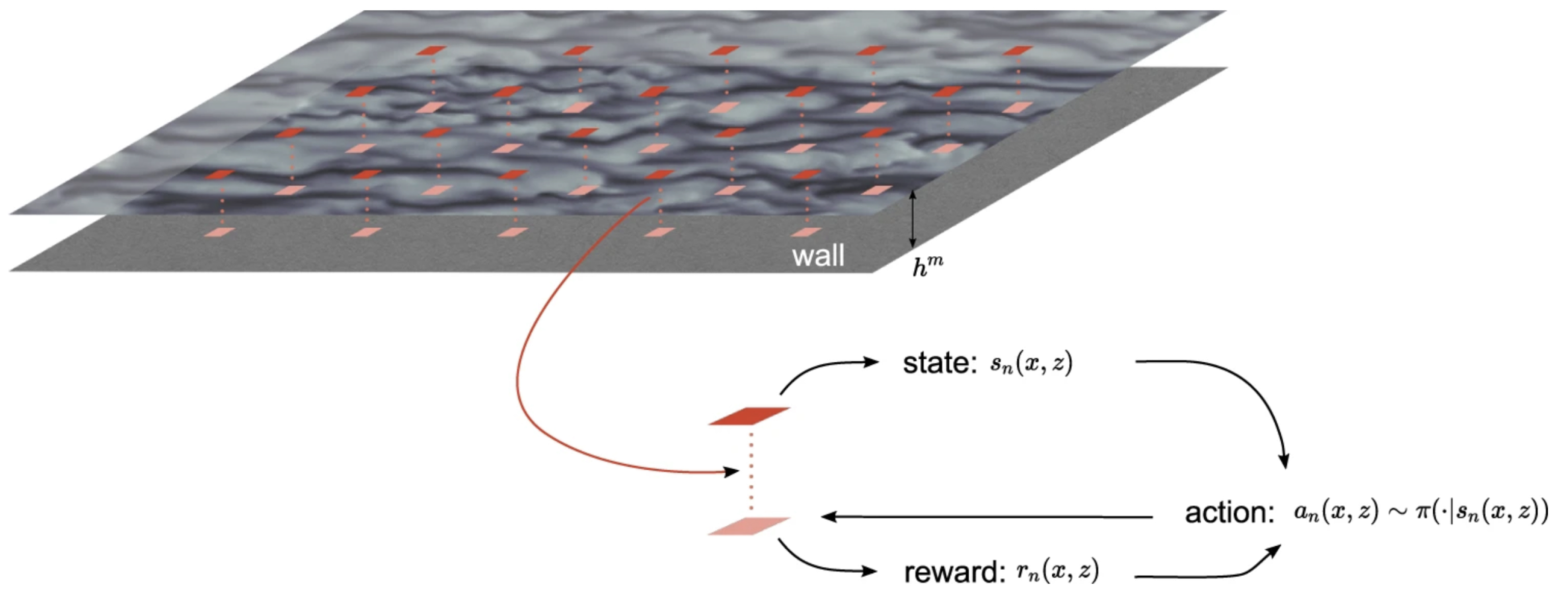
Note that reinforcement learning is a type of machine learning framework that employs artificial intelligence in complex applications, such as self-driving cars, and more. Bae and Koumoutsakos [11] proposed the multi-agent reinforcement learning method to approximate the subgrid-scale quantity $c_s(\mathit{x},t)$. To briefly illustrate the NN-based reinforcement learning of the near-wall turbulence, we illustrate the conceptual framework in Figure 1. In this approach, we consider several fluid parcels to act like agents learning the flow environment at each time step. Each agent performs an action according to a desired wall-modeled LES (see [28]) and receives a scalar reward to update the wall shear stress. In order for the reinforcement learning of agents to be universally applicable, the machine learning algorithm establishes a relationship between the wall friction velocity and the wall shear stress (see [11]).

3.2. Solving PDEs with Neural Networks

The application of NNs to construct numerical solution methods for PDEs dates back to the early 1990s [64,65,66]. Recently, physics-informed neural networks (PINN) [67] have initiated a surge of ensuing research activity in the deep learning of nonlinear PDEs. The PINN approach employs NNs to solve PDEs in the simultaneous space-time domain. Here, we illustrate the PINN method for approximating the solution $u:[0,T]\times \Omega \to \mathbb{R}$ of the following evolutionary PDE [68]:

$$\frac{\partial u}{\partial t}+\mathcal{N}\left(u\right)=0(x,t)\in \Omega \times [0,T]$$

(11)

subject to boundary conditions $u(x,t)=u_b(x,t)$ for $(x,t)\in (0,T)\times \partial \Omega$ and initial conditions $u(x,0)=u_0:\Omega \to \mathbb{R}$. Using the neural network approach, we find the best parameter w for the approximation $u_w(x,t)\approx u(x,t)$, where the initial condition and the boundary conditions provide training data. Then, we minimize the residual (or loss) $\mathcal{R}\left[u_w\right]:={\partial }_t{u}_w-\mathcal{N}\left[u_w\right]$ over a set of scattered grid points in the simultaneous space-time domain. To construct a solution by a purely data-driven approach, PINN considers a set of N state–value pairs ${\left\{(x_i,t_i,u_i)\right\}}_{i=1}^N$, where $u_i:=u(x_i,t_i)$ is unknown. Then, we search for a neural network approximation $u_w(x_i,t_i)$ and find the best fit parameter w such that $u_w(x_i,t_i)=u(x_i,t_i)$ for $i=1,\dots ,N$. Finally, $u_w(x,t):\Omega \times [0,T]\to \mathbb{R}$ denotes a solution realized by the neural network using the optimal values of the parameter w. Note that the PINN approach does not require past solutions as training data. Instead of minimizing the standard error $|u_w(x_i,t_i)-u(x_i,t_i)|$, the PINN method takes the PDE as the underlying physics and minimizes the least square residual $\left|\right|\mathcal{R}\left[u_w\right]{\left|\right|}_2^2$ to find the optimal values of the parameter w. Several publications [69] reviewed the application of the PINN method to solve the Navier–Stokes equations. For incompressible flows, PINNs form the neural network approximation of each velocity component and pressure by minimizing the residual of Navier–Stokes equations on a set of space-time collocation points.

3.3. Remark

In this section, we have briefly reviewed machine learning frameworks to accelerate the LES of turbulent flows. Machine learning of new subgrid models from high-resolution flow fields is a promising approach, but such artificial intelligence applications have been prone to instabilities, and their performance on different grid spacings has not been investigated. We illustrate the neural network pathway to turbulence modeling. The universal approximation theorem implies that neural networks can find appropriate weights w and minimizes the bias b to represent a wide variety of interesting functions, such that [70]

$$y=f\left(x\right)\approx wx+b.$$

The NN approach is a powerful framework that we can adapt to the computation of various turbulent quantities.

We show that the PINN approach can directly solve a nonlinear PDE. Nevertheless, solving the Navier–Stokes equations at very large Reynolds numbers require PINNs to incorporate a suitable turbulence modeling scheme, which is currently a work in progress. For solving Equation (11), the PINN approach has the flexibility of incorporating subgrid-scale terms through supervised or reinforcement learning approaches. Note that a principle of machine learning is to provide a probability distribution $\sigma (x,y)$ of input–output pairs, while minimizing the loss function (9). Thus, we have enough flexibility to “inform” the underlying “physics” as we construct a universal approximation of fluid flows by neural networks.

4. Wavelets in Computational Fluid Dynamics

4.1. Background

The wavelet method evolved as a nonlinear approximation of the critical information in high-dimensional systems. The wavelet-based CFD techniques are efficient algorithms that map a high-dimensional fluid dynamics phenomena onto a low-dimensional manifold. Our classical CFD approach is not suitable to deal with the large number of the degrees of freedom of turbulent flows. The wavelet method projects the turbulent flow onto a low-dimensional manifold to capture the energy containing motion with a relatively small number of the wavelet modes (or grid points). The wavelet transform is a convolution with wavelets, which is translation covariant. It is thus suitable to extract multiscale energy containing eddies of turbulent motions [6].

In the late 1980s, Farge and Rabreau [71] introduced for the first time the novel idea of wavelet-based turbulence modeling (see [3,72,73,74]). Over the last decade, a number of new developments have been made. The wavelet method in CFD has evolved in two directions. First, the coherent vortex simulation (CVS) methodology is based on the idea that vortex stretching drives the energy cascade phenomena in turbulent flows [36,38,75,76]. Since nonlinear terms of the Navier–Stokes equations represent vortex stretching, the vorticity is an appealing candidate for turbulence modeling. Farge et al. [72] have discussed more details in this direction. The second approach is the adaptive wavelet collocation method (AWCM) that generalizes the classical turbulence modeling toward a new direction of the wavelet-based CFD techniques. AWCM follows the hypothesis that the energy cascade occurs through a hierarchical breakdown of eddies in a localized manner [77]. Some of the recent developments of AWCM include wavelet adaptive DNS (WA-DNS), wavelet adaptive LES (WA-LES), wavelet adaptive RANS (WA-RANS), wavelet adaptive detached-eddy simulation (WA-DES), and wavelet adaptive climate model (WAVTRISK) [35,78,79,80,81].

Here, we want to highlight the fundamental differences between the CVS and AWCM in the context of turbulent flows. CVS treats vortex tubes as “sinews” of turbulence [4]. Vortex tubes with diameters between the Kolmogorov micro scale and Taylor micro scale are usually surrounded by the strain field [4]. When a vortex tube is stretched, its circulation is conserved, and it exerts a tensile stress onto the surrounding strain, which cascades energy toward smaller scales. Since the tube-like vortices occupy a relatively small fraction ($\sim 1\%$) of the total volume, a relatively small number of grid points is necessary to account for a much larger fraction (10–20%) of the turbulence energy dissipation. The main strategy of CVS is thus to employ wavelets for projecting coherent vortices onto a low-dimensional manifold and to solve the Navier–Stokes equations on a wavelet basis.

The AWCM is based on the assumption that the energy dissipation is confined to high-wavenumber Fourier modes that are highly localized, whereas the injection of energy is confined to the low-wavenumber Fourier modes. Thus, AWCM employs wavelets to dynamically adapt the computational grid to capture the localized energy dissipation rates. AWCM requires a subgrid-scale model (e.g., WA-LES) unless the smallest resolved scale is approximately the same as the dissipation scale (e.g., WA-DNS). This approach is not compatible with the local production of small-scale vorticity in boundary layers or shear layers. Nevertheless, simulations of homogeneous isotropic turbulence show that the Reynolds number scaling of CVS, $\mathcal{O}\left(\mathcal{R}{e}^3\right)$, is slightly higher than that of AWCM (specifically WA-LES), $\mathcal{O}\left(\mathcal{R}{e}^{2.75}\right)$. Recently, Mehta et al. [17], Ge et al. [8], and De Stefano and Vasilyev [35] covered a detailed review of turbulence modeling by the AWCM approach. Such studies primarily focused on the promise of wavelet compression and grid adaptation. Below, we provide a technical overview of the above discussion regarding vortex stretching. Readers interested in more details are referred to (in particular chapter 5 of) Davidson [4].

4.2. Coherent Structure Extraction by the CVS and the AWCM Methods

Considering the velocity $\mathit{u}$ as a diagnostic variable via vorticity $\mathit{\omega }=\mathbf{\nabla }\times \mathit{u}$, three-dimensional Navier–Stokes equations read as follows:

$$\frac{\partial \mathit{\omega }}{\partial t}+\mathit{u}·\mathbf{\nabla }\mathit{\omega }=\mathit{\omega }·\mathbf{\nabla }\mathit{u}+\frac{1}{\mathcal{R}e}{\mathbf{\nabla }}^2\mathit{\omega }.$$

(12)

Using the wavelet-based solution $\overline{\mathit{\omega }}$ of Equation (12) in $\overline{\mathit{\omega }}=\mathbf{\nabla }\times \overline{\mathit{u}}$, we find a wavelet-filtered velocity $\overline{\mathit{u}}$, which is an approximation to the solution of the wavelet-filtered Navier–Stokes equations, Equations (2) and (3).

To extract coherent structures by the CVS approach, we split each snapshot of a turbulent flow into two parts. The wavelet-filtered vorticity $\overline{\mathit{\omega }}\left(\mathit{x}\right)$ is given by the inverse wavelet transform applied to wavelet coefficients whose modulus is larger than the threshold ${\epsilon }_{\mathrm{opt}}=\sqrt{4\mathcal{Z}ln\mathcal{N}/3}$, where $\mathcal{Z}={(1/2)\int \left|\mathit{\omega }\right|}^{2}d\mathit{x}$ is the total enstrophy. The residual part ${\mathit{\omega }}^{\prime }=\mathit{\omega }\left(\mathit{x}\right)-\overline{\mathit{\omega }}\left(\mathit{x}\right)$ represents the incoherent background. It is worth mentioning that the CVS decomposition follows one of the best known mathematical results, due to Foias and Temam [82], that the regularity and uniqueness of the velocity are guaranteed up to a finite time if the enstrophy ($\mathcal{Z}$) of the flow remains bounded. According to Donoho [83], the optimal wavelet thresholding corresponds to negligible subfilter-scale stresses (via Leonard decomposition). By the Helmholtz vortex theorem, the vortex-flux through a vortex tube is conserved as the tube is stretched, and the strength of a stretched vortex increases in direct proportion to its length [4].

Taylor [84] considered experimental data to analyze the production of enstrophy in decaying turbulence generated from wind-tunnel measurements of the velocity. Based upon the equation for enstrophy production, Taylor [84] argued that enstrophy will be created when the mean rate of vortex stretching is positive and exceeds the mean destruction of enstrophy by viscosity. In the AWCM approach, we consider the wavelet-filtered velocity $\overline{\mathit{u}}$ to extract coherent vortices $\overline{\mathit{\omega }}=\mathbf{\nabla }\times \overline{\mathit{u}}$ and solve the wavelet-filtered momentum Equations (2) and (3), instead of directly solving Equation (12). Here, the cumulative effect of discarding all wavelet modes is associated with the total energy $E={(1/2)\int \left|\mathit{u}\right|}^{2}d\mathit{x}$ instead of the total enstrophy, $\mathcal{Z}$ [80,85]. Note also that AWCM solves the momentum Equations (2) and (3) considering the subfilter-scale stress terms [8,80], where the effects of the subfilter-scale stress ${\tau }^s=[{\overline{u_{i}u}}_j-{\overline{u}}_i{\overline{u}}_j]$ is not negligible [85,86]. A comparison of the evolution of enstrophy between the CVS and AWCM approaches is crucial in the context of enstrophy production by vortex stretching.

Applying the curl operator onto Equation (3), we obtain the vorticity equation associated with the AWCM approach, which leads to the following form of the wavelet-filtered enstrophy equation:

$$\frac{\partial }{\partial t}\left(\frac{1}{2}{\left|\overline{\mathit{\omega }}\right|}^2\right)={\overline{\mathit{\omega }}}^T\mathcal{S}\overline{\mathit{\omega }}-\frac{1}{\mathcal{R}e}{|\mathbf{\nabla }\overline{\mathit{\omega }}|}^2-\underset{\mathrm{subgrid}\mathrm{enstrophy}}{\underbrace{\left[\mathbf{\nabla }·\left({\tau }^s-\frac{1}{3}\mathrm{tr}{\tau }^s\right)\right]·(\mathbf{\nabla }\times \overline{\mathit{\omega }})}}.$$

(13)

The first term on the righthand side of Equation (13) represents inertial-range vortex-stretching. The last term in Equation (13) (denoted by “subgrid enstrophy”) represents the enstrophy flux to unresolved scales, which is due to the subgrid-scale turbulence modeling because the AWCM solves Equation (3). Removing the last term from Equation (13) provided the enstrophy evolution of the CVS method. Clearly, in Equation (13), the last term accounts for the enstrophy production associated with the subgrid model (4). In other words, Equation (13) suggests that a primary role of the subgrid model (in WA-LES) is to dissipate the subgrid-scale production of enstrophy [82]. Moreover, the CVS method directly accounts for the conservation of circulations, which is essential to ensure that the mean rate of positive vortex-stretching causes the forward energy cascade to small scales.

4.2.1. CVS Modes of Near-Wall Dynamics

The CVS method employs a nonlinear approximation that designs a good nonlinear dictionary, and finds the optimal approximation as a linear combination of $\mathcal{N}$ elements of the dictionary. The main goal is to identify the CVS modes leading to the best $\mathcal{N}$-term approximation of a turbulent flow. CVS is a two-stage process. First, we identify the dictionary of wavelets extracting hidden information of the vorticity field. Second, we extract the CVS modes by finding the best wavelets associated with the dominant vortical structures.

Here, we briefly illustrate the CVS method for capturing the near-wall vortices from the DNS data of a turbulent channel flow. The technical details of the channel flow simulation are given by Sakurai et al. [87]. Applying the CVS method onto the vorticity field, we extract the coherent flow structure in the near-wall region. It is worth mentioning that standard techniques, such as the Q-criteria, identify the region where vorticity dominates over the strain. A region of negative ${\lambda }_2$, the second largest eigenvalue of the tensor ${\mathcal{S}}_{ik}{\mathcal{S}}_{kj}+{\mathcal{R}}_{ik}{\mathcal{R}}_{kj}$, captures the vortical flow structures. Standard vortex identification criteria use the velocity gradient tensor in physical space. In contrast, the CVS modes extract the hidden patterns of the vorticity field in Fourier space.

At the top of Figure 2, we show the total vorticity $|\overline{\mathit{\omega }}|$ (green) of the DNS of $256\times 256\times 2048$ (i.e., $\approx 130$ million) grid points. Then, wavelet decomposition was applied to the total vorticity. In the middle of Figure 2, we show the vorticity $|\overline{\mathit{\omega }}|$ (red) of the CVS modes. We observe that these vortices have been captured by about $7\times {10}^6$ of the CVS modes (Figure 2, red). This number of CVS degrees of freedom is only about $0.55$% of the original number of grid points. The incoherent vorticity is the residual $|\mathit{\omega }-\overline{\mathit{\omega }}|$, which is shown at the bottom of Figure 2 (blue). The CVS modes capture the coherent flow, which retains $99.9$% of the total energy and $99.7$% of the total enstrophy.

4.2.2. The POD Modes of Coherent Structures

In the late 1960s, Lumley [2] introduced the POD method, which is an orthogonal decomposition of a function, $u(x,t):[a,b]\times [0,T]\to \mathbb{R}$, given by

$$u(x,t)=\sum _{k=0}^{\infty }{c}_k\left(t\right){\phi }_k\left(x\right).$$

(14)

The decomposition (14) is said to be complete if it converges to all $u(x,t)\in L^2[a,b]$ for all $t\in [0,T]$ (some texts refer to this a generalized Fourier series of functions satisfying periodic boundary conditions). The Bessel’s inequality and the Parseval’s equality

$$\sum _{k=0}^{\infty }{c}_k^2\left|\right|{\phi }_k{\left(x\right)\left|\right|}^2\le {\left|\right|u\left|\right|}^2{<\infty \mathrm{and}\left|\right|u\left|\right|}^2=\sum _{k=0}^{\infty }{c}_k^2\left|\right|{\phi }_k{\left(x\right)\left|\right|}^2\le {\left|\right|u\left|\right|}^2,\mathrm{respectively},$$

guarantee that a finite number of coefficients $c_k=\langle u,{\phi }_k\rangle /\left|\right|{\phi }_k{\left|\right|}^2$ is sufficient for the best approximation of all $u\in L^2[a,b]$ for all $t\in [0,T]$ [88].

The POD is a widely used unsupervised machine learning technique to study turbulent flows [89]. For 3D turbulent flows, the POD method provides a data-driven basis ${\left\{{\phi }_k\left(\mathit{x}\right)\right\}}_{k=1}^{\mathcal{N}}$ with a near-optimal dimension $\mathcal{N}$, which represents the spatial coherence of the flow kinematics, while the time evolution of the coefficients ${\left\{c_k\left(t\right)\right\}}_{k=1}^{\mathcal{N}}$ captures the low-dimensional coherent dynamics. Thus, the POD method essentially offers an optimal low-dimensional approximation of high-dimensional fluid data using an orthogonal basis in a certain least-squares optimal sense [90]. In the context of the Germano identity [91] (and the Leonard decomposition), the POD method extracts most of the resolved turbulence kinetic energy. Recent works [92,93,94,95,96] demonstrate the potential of the POD method in capturing complex turbulent flows, but its application to turbulence modeling is relatively new [97].

Here, we employ the best approximation using the POD modes to formulate the Leonard decomposition of a turbulent flow. Consider the velocity snapshots, $\mathcal{U}=\left[\tilde{u}({\mathit{x}}_i,t_j)\right]$, and construct a decomposition of the form $\mathcal{U}=\overline{\mathcal{U}}+{\mathcal{U}}^{″}$, where $\overline{\mathcal{U}}$ contains most of the (turbulence kinetic) energy such that $\left|\right|{\mathcal{U}}^{″}{\left|\right|}_1$ is minimized. Such a decomposition would minimize the following Lagrangian

$$L(\overline{\mathcal{U}},{\mathcal{U}}^{″},V)=\left|\right|\overline{\mathcal{U}}{\left|\right|}_{\ast }+\lambda \left|\right|{\mathcal{U}}^{″}{\left|\right|}_1+V^T(\mathcal{U}-\overline{\mathcal{U}}-{\mathcal{U}}^{″})+\frac{\eta }{2}\left|\right|\mathcal{U}-\overline{\mathcal{U}}-{\mathcal{U}}^{″}{\left|\right|}_F^2$$

(15)

to extract the energy containing motion captured by the POD modes. Note that minimizing the nuclear norm $\left|\right|·{\left|\right|}_{\ast }$ ensures maximization of the resolved turbulence kinetic energy (i.e. data variance) over a low-dimensional subspace. In addition, minimizing the norm $\left|\right|{\mathcal{U}}^{″}{\left|\right|}_1$ aims to capture the intermittency of turbulence fluctuations. Based on the POD method, we compute the Leonard stress ${\tau }_{ij}^L={\overline{{\tilde{u}}_i\tilde{u}}}_j-{\overline{\tilde{u}}}_i{\overline{\tilde{u}}}_j$ (see [97]). Minimizing the Lagrangian Equation (15) for a short-time snapshot, the POD method captures the most energy containing coherent structures with respect to a cutoff time-scale $\alpha {\Delta }_t$ that is equivalent to a spatial cutoff scale $\alpha \Delta$, where $\alpha \ge 1$ and ${\Delta }_t$ is the turnover time units of the smallest resolved eddies (see Pruett et al. [98]). We know that the commutativity (of filtering and differentiation) is natural for a temporal filter, which remains problematic for spatial ones. The temporally filtered Navier–Stokes equations remain frame-invariant under the Galilean group of transformations [19,98]. Thus, minimizing the Lagrangian Equation (15) must faithfully resolve a significant fraction of the subfilter-scale stress ${\tau }_{ij}^s$. However, a sharp cutoff of frequencies does not translate into sharp cutoff of spatial scales [19,97]. Thus, we may better understand relatively difficult turbulent flows (e.g., [96,99]) by advancing the mixed-subgrid models that combine a temporal filtering approach with a spatially filtered subgrid model. Combining a spatial filtering process with the POD method, we get

$${\tau }_{ij}^s\approx \underset{{\tau }_{ij}^L}{\underbrace{{\overline{{\tilde{u}}_i\tilde{u}}}_j-{\overline{\tilde{u}}}_i{\overline{\tilde{u}}}_j}}+\underset{{\tau }_{ij}}{\underbrace{\overline{{\overline{u}}_i{u}_j^{\prime \prime }}+\overline{u_i^{\prime \prime }{\overline{u}}_j}-{\overline{{\overline{u}}_i\overline{u}}}_j}}.$$

(16)

Equation (16) takes the standard form of a mixed model [18], where the Leonard stress ${\tau }_{ij}^L$ is obtained through the POD method and subgrid-scale stress ${\tau }_{ij}$ is obtained through a classical approach. The linear combination of the Leonard (resolved) stress (${\tau }_{ij}^L$) with the subgrid- scale stress (${\tau }_{ij}$) improves the prediction of the true subfilter-scale stress (${\tau }_{ij}^s$). Note that Kang et al. [100] proposed a mixed-subgrid-scale model using the NN approach and tested the performance by simulating isotropic turbulence and turbulent channel flow. Within the scope of the present review, we find that the underlying premise of considering the POD method in LES is that the low-dimensional POD of short-time snapshots also attenuates the small-scale fluctuations by time-domain filtering (see [89]). To date, the literature is not fully clear about the computational improvement of considering the POD method in LES. A more fundamental understanding of the relationship between the time-domain filtering by the POD and the attenuation of high-wavenumber content by the wavelet method would take a major step forward for the wavelet-based high-fidelty LES methodology.

Let us now briefly review the wavelet method and the POD method for dimensionality reduction while extracting coherent structures. Here, we consider the velocity snapshots $\mathcal{U}$ for a two-dimensional flow past a circular cylinder at $\mathcal{R}e=\mathrm{14,440}$ [101]. A column of $\mathcal{U}\in {\mathbb{R}}^{2N\times M}$ consists of two velocity components ${[u(x_i,y_j,t_n),v(x_i,y_j,t_n)]}^T$ at N grid points $(i,j)$ and n-th time step. Consider the one-dimensional wavelet transform of each row of $\mathcal{U}$. The wavelet transform produces coefficients that contain energetic information of the relative local contribution of various frequency bandwidths at each level of wavelet transform. Figure 3a shows the energy distribution of wavelet components. The cumulative energy at each successive level of wavelet decomposition is also shown.

We have compared the relative energy per wavelet mode with that of the POD modes. Figure 3b shows the energy distribution of POD modes. Figure 3 compares the energy distribution of wavelet modes (Figure 3a) and POD modes (Figure 3b). The first four wavelet components contain $88\%$ of the total kinetic energy. The wavelet components of levels 1 and 2 makes the largest contribution, accounting for $32\%$ and $45\%$ energy, respectively. The first four POD modes are the most energetic, containing $80\%$ of the total kinetic energy. The first and the second POD modes contribute $41\%$ and $32\%$ energy, respectively. The energy distribution of first two wavelet components is similar to the first two POD modes [102].

4.3. Space-Time Wavelet and Neural Networks

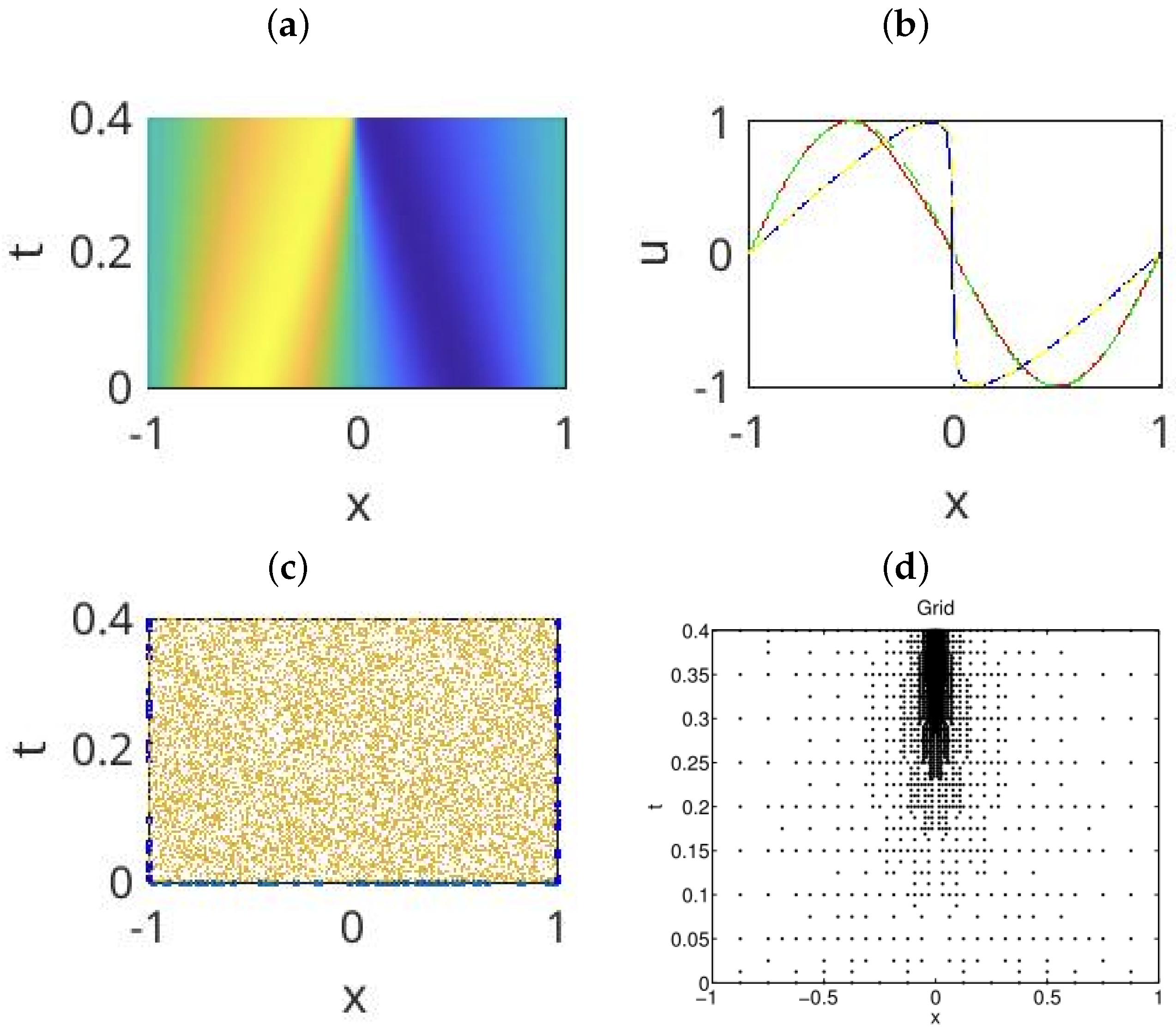
This section reviews the connection between the wavelet transforms and the machine learning methods for simulating turbulent flows [103,104]. In the last few decades, many researchers focused on the one-dimensional coneptual model of turbulence using the Burgers equation. Here, we consider the one-dimensional Burgers equation to illustrate both the space-time adaptive wavelet method [105] and the PINN method [68] for solving PDEs. The wavelet method finds the optimal number of the wavelet modes to formulate the best approximation $u_w(x,t)\approx u(x,t)$ of the solution. Each wavelet mode (indicated by the subscript ${}_w$) is associated with a grid point. Thus, discarding a wavelet mode discards the corresponding grid point. We minimize the wavelet-based residual ${\mathcal{R}}_w$ over an essential set of the collocation points, the number of which is usually small. Interested readers may find a technical details of the space-time wavelet method given by Alam et al. [105].

This review considers the PINN method in Python programming framework using the TensorFlow environment. Our code has been adapted from Raissi et al. [68]. Note that the PINN method finds the best approximation $u_w(x,t)\approx u(x,t)$ of the solution by finding the optimal values of the parameter w. Here, we have kept the same symbol ‘w’ to denote wavelet modes and neural networks weights, respectively. Classical machine learning minimizes the residual $\mathcal{R}\left[u_w\right]$ given by Equation (9). However, the underlying premise of PINNs is that the boundary condition and the differential operators simulatneously define the residual $\mathcal{R}\left[u_w\right]$ to ‘inform’ the ‘physics’ of the problem while training neural networks. In other words, PINNs find the solution on a (training) set of collocation points in the simultaneous space-time domain.

Figure 4a,b compares the solution $u(x,t)$ between the two methods. Figure 4c,d compares, respectively, the collocation points used by the PINN and the space-time wavelet methods. We see from Figure 4c that PINNs aim to optimize the values of the parameter w on a set of randomly chosen training samples. There is no requirement to adjust the location or the number of training samples. Figure 4d shows that the space-time wavelet method clusters the collocation points as it learns the steep gradient of the solution.

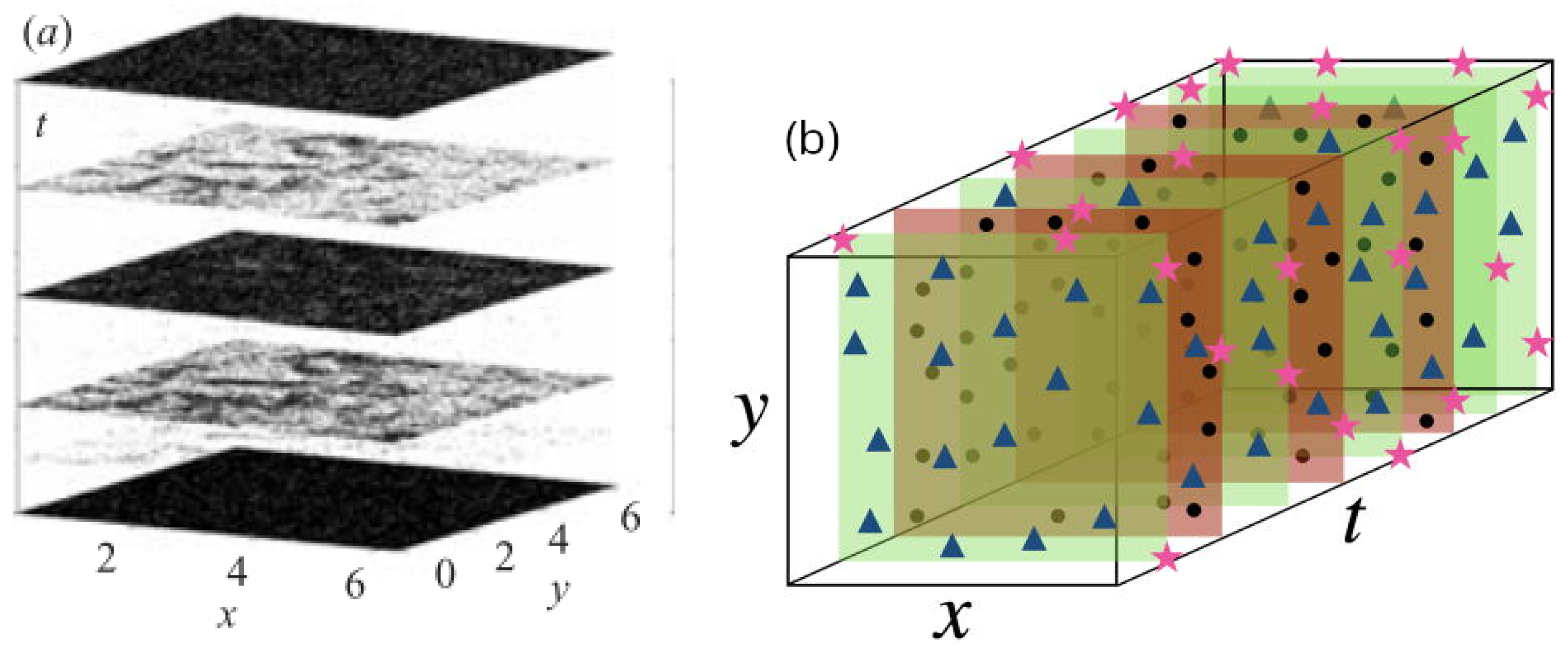
Here, we briefly discuss the application of the space-time wavelet transforms and the PINN for simulating two-dimensional turbulence. First, we discuss the supervised learning of 2D turbulence by minimizing the wavelet-based residual (or loss). Figure 5a shows the locations ($x,y,t$) of flow samples in the space-time domain. We consider 3D tensor-product wavelet transform and minimize the equation loss (or residual) to find a set of best wavelet coefficients. The clustering of the collocation points shows that the wavelet transforms dynamically adapt $\mathcal{N}$ samples ${\{x_i,y_i,t_i,u(x_i,y_i,t_i)\}}_{i\le \mathcal{N}}$ [103] to learn fluid velocity $u(x,y,t)$ at every point of the domain [9]. According to Bishop [9] and Raissi et al. [67], the space-time wavelet method is like a physics-informed supervised machine learning, which takes a set of inputs ${\{x_i,y_i,t_i\}}_{i\le \mathcal{N}}$ and a set of output ${\left\{u(x_i,y_i,t_i)\right\}}_{i\le \mathcal{N}}$, finding the best weights that minimize the ${\ell }_0$ or ${\ell }_1$ norm of the wavelet coefficients and the corresponding residual. In this particular example, the minimization of the equation loss (by the gradient descent method) was regularized by minimizing the ${\ell }_0$ norm of wavelet coefficients. Kevlahan et al. [103] observed that the space-time wavelet method accurately reproduces DNS results.

Figure 5b shows the collocation points that we randomly chose to train the PINNs model. However, the main challenge of PINNs to reproduce DNS results of turbulent flows arises from the need for a large amount of training data [104]. To date, we do not know the Reynolds number scaling of PINN-based simulation of turbulent flows, nor do we know whether PINN-based methods would capture the global behavior of turbulence.

Arzani et al. [106] and Kag et al. [104] observed that sparse collocation points are appropriate for training PINNs models. Injecting the sparse nature of underlying physics through DNS data or spectral decomposition helps improve the results of PINN-based turbulence simulation [104]. Such a remarkable finding for the PINNs method motivates us to take advantage of the space-time wavelet method and the PINN method. According to Kag et al. [104], capturing turbulent flow physics within PINNs may lead to a potentially robust turbulence modeling approach.

5. Conclusions and Future Direction

Wavelet-based turbulence modeling is a research topic more than 30 years old. While many researchers have thoroughly investigated the AWCM and the CVS methods, their applicability remains limited by the underlying mathematical complexity of wavelet transforms [35,107]. The CVS method has evolved around the Taylor hypothesis that vortex-stretching is a primary mechanism for the energy cascade. In contrast, the AWCM follows the Richardson hypothesis [77] and assumes that the fidelity of subgrid models depends on the local grid refinement to ensure that subgrid scales are approximately isotropic. Thus, both the AWCM and the CVS can drastically reduce the computational complexity of the turbulent flow simulation [17,35,107]. A large number of articles have demonstrated wavelet-based RANS, DES, and LES techniques for the numerical simulation of compressible and incompressible flows (e.g., the Ref. in [17]).

Similar to supervised (and reinforment) machine learning, wavelet transforms have the ability to learn the invariant manifold, which accounts for the low-dimensional coherence of the turbulent flow dynamics [6,83,89]. Both the CVS and the AWCM are learning algoritms that optimize the wavelet coefficients in order to minimize the average reconstruction error on the adaptively chosen training samples [3,7]. The wavelet transforms separate scales, followed by a nonlinear threshold (or activation), and ultimately learn the invariant manifold of the high-dimensional input data, such as velocity fields in turbulent flows. It is worth mentioning that deep neural networks are intelligent computational architectures that are promising in the regression and classification of big data problems [108]. The striking similarities between wavelet transforms and machine learning indicate a potential cross-fertilization and the development of a common mathematical framework, particularly in the study of turbulence.

Recently, the applications of wavelet transforms and machine learning in turbulence modeling have emerged as a promising area of investigation [10,17]. This review highlights two primary challenges in developing machine learning techniques for subgrid models of turbulence. First, in turbulence modeling, achieving an optimal low-dimensional representation of both the nonlinear dynamics and the large-scale turbulent motion is important. For instance, this concept is a principal hypothesis of LES, where (implicit) filtering captures the low-dimensional, coarse-grained flow features. In most applications of machine learning, the number of training samples would grow linearly with the dimensionality of the system (see Brunton et al. [10] and the references therein). Such a curse of dimensionality is a bottleneck for machine learning of high-Reynolds-number turbulence, where the number of degrees of freedom scales like $\mathcal{R}{e}^3$. Second, turbulence is highly sensitive to changes in geometry, flow parameters, and boundary conditions. The lack of generalization of machine learning (including the reinforcement learning) limits the broader applicability of such methods in practical engineering and scientific applications.

Summary Points and Future Tasks

• Over the past decades, the fluid dynamics community has explored unsupervised machine learning [10] and cutting-edge first-principles-based (LES) techniques [22] to understand turbulent flows. Recent progresses in machine learning techniques offer valuable insights in the study of turbulent flows [11,104,109]. By bridging machine learning and first-principles-based approaches, we can uncover new physical mechanisms, symmetries, invariants, and constraints from fluid data.
• Wavelet transforms naturally entail machine learning algorithms that learn the multiscale physics necessary for modeling, optimization, and control of turbulent flows [6,7]. Classical supervised machine learning is a high-dimensional interpolation problem that learns the optimal map between inputs and outputs [9]. Limited availability of the high-quality (“ground truth”) output of turbulence quantities (such as stress, eddy viscosity, etc.) hinders the application of such machine learning to solve turbulence problems.
• Physics-informed neural networks emerged as a new subclass of supervised machine learning to reduce the requirement of the large amount of high-quality data in lieu of first principles governing equations for the desired physics [67,104,109]. However, such a method of combining machine learning and first-principles-based approaches still requires clipping with additional high-quality data [104] or a model for turbulence and wall stresses [109] to deal with the multiscale challenges of turbulence.

Recent developments in the applications of machine learning in turbulence modeling aim to speed up the computational cost of solving the Navier–Stokes equations. In other words, machine learning would deal with the near-wall and the subgrid-scale phenomena, while first principles account for the significant or large-scale processes (e.g., Bae and Koumoutsakos [11]). A formal analysis of the speed-up of CFD calculations with machine learning requires further investigations. Some studies indicate a 20% speed-up of CFD calculations if machine learning takes care of some of the costly elements of turbulence modeling. In contrast, wavelet methods are efficient to drastically reduce the number of computational elements in CFD calculations [7,17,103]. The space-time adaptive wavelet collocation method (e.g., Alam et al. [105]) is similar to the recent developments of physics-informed neural networks proposed by Raissi et al. [68]. Clearly, there are potential new research directions in the applications of neural networks and wavelet transfroms, which may benefit our understanding of many unresolved problems of fluid turbulence. Finally, this brief review of wavelet transforms and machine learning opens new questions. However, the potential consequences of combining both approaches require further investigations.

References

- Kolmogorov, A.N. The Local Structure of Turbulence in the Incompressible Viscous Fluid for very Large Reynolds Number. C. R. Acad. Sci. U.S.S.R. 1941, 30, 301–306. [Google Scholar]
- Lumley, J.L. The structure of inhomogeneous turbulent flows. Atmospheric Turbulence and Radio Wave Propagation. In Proceedings of the International Colloquium, Moscow, Russia, 15–22 June 1967. [Google Scholar]
- Farge, M. Wavelet transforms and their application to turbulence. Annu. Rev. Fluid Mech. 1992, 24, 395–457. [Google Scholar] [CrossRef]
- Davidson, P.A. Turbulence—An Introduction for Scientists and Engineers; Oxford University Press: Oxford, UK, 2004. [Google Scholar]
- Vinuesa, R.; Brunton, S. Enhancing computational fluid dynamics with machine learning. Nat. Comput. Sci. 2022, 2, 358–366. [Google Scholar] [CrossRef]
- Mallat, S. A Wavelet Tour of Signal Processing; Academic Press: Cambridge, MA, USA, 2009. [Google Scholar]
- Schneider, K.; Vasilyev, O.V. Wavelet Methods in Computational Fluid Dynamics. Annu. Rev. Fluid Mech. 2010, 42, 473–503. [Google Scholar] [CrossRef] [Green Version]
- Ge, X.; De Stefano, G.; Hussaini, M.Y.; Vasilyev, O.V. Wavelet-Based Adaptive Eddy-Resolving Methods for Modeling and Simulation of Complex Wall-Bounded Compressible Turbulent Flows. Fluids 2021, 6, 331. [Google Scholar] [CrossRef]
- Bishop, C.M. Pattern Recognition and Machine Learning (Information Science and Statistics); Springer: Berlin/Heidelberg, Germany, 2006. [Google Scholar]
- Brunton, S.L.; Noack, B.R.; Koumoutsakos, P. Machine Learning for Fluid Mechanics. Annu. Rev. Fluid Mech. 2020, 52, 477–508. [Google Scholar] [CrossRef] [Green Version]
- Bae, H.J.; Koumoutsakos, P. Scientific multi-agent reinforcement learning for wall-models of turbulent flows. Nat. Commun. 2022, 13, 1–9. [Google Scholar]
- Pope, S.B. Turbulent Flows; Cambridge University Press: Cambridge, UK, 2000. [Google Scholar]
- Wang, J.X.; Wu, J.L.; Xiao, H. Physics-informed machine learning approach for reconstructing Reynolds stress modeling discrepancies based on DNS data. Phys. Rev. Fluids 2017, 2, 034603. [Google Scholar] [CrossRef] [Green Version]
- Singh, A.P.; Medida, S.; Duraisamy, K. Machine-Learning-Augmented Predictive Modeling of Turbulent Separated Flows over Airfoils. AIAA J. 2017, 55, 2215–2227. [Google Scholar] [CrossRef]
- Maulik, R.; San, O.; Rasheed, A.; Vedula, P. Subgrid modelling for two-dimensional turbulence using neural networks. J. Fluid Mech. 2019, 858, 122–144. [Google Scholar] [CrossRef] [Green Version]
- Jin, X.; Cai, S.; Li, H.; Karniadakis, G.E. NSFnets (Navier-Stokes flow nets): Physics-informed neural networks for the incompressible Navier-Stokes equations. J. Comput. Phys. 2021, 426, 109951. [Google Scholar] [CrossRef]
- Mehta, Y.; Nejadmalayeri, A.; Regele, J.D. Computational Fluid Dynamics Using the Adaptive Wavelet-Collocation Method. Fluids 2021, 6, 377. [Google Scholar] [CrossRef]
- Bardina, J.; Ferziger, J.; Reynolds, W. Improved subgrid-scale models for large-eddy simulation. In Proceedings of the 13th Fluid and Plasma Dynamics Conference, Snowmass, CO, USA, 14–16 July 1980. [Google Scholar]
- Oberle, D.; Pruett, C.D.; Jenny, P. Effects of time-filtering the Navier–Stokes equations. Phys. Fluids 2023, 35, 065112. [Google Scholar] [CrossRef]
- Smagorinsky, J. General Circulation Experiments with the Primitive Equations. Mon. Weather Rev. 1963, 91, 99. [Google Scholar] [CrossRef]
- Lilly, D.K. A proposed modification of the Germano subgrid scale closure method. Phys. Fluids 1992, 4, 633–635. [Google Scholar] [CrossRef]
- Moser, R.D.; Haering, S.W.; Yalla, G.R. Statistical Properties of Subgrid-Scale Turbulence Models. Annu. Rev. Fluid Mech. 2021, 53, 255–286. [Google Scholar] [CrossRef]
- Sarghini, F.; de Felice, G.; Santini, S. Neural networks based subgrid scale modeling in large eddy simulations. Comput. Fluids 2003, 32, 97–108. [Google Scholar] [CrossRef]
- Meneveau, C. Lagrangian Dynamics and Models of the Velocity Gradient Tensor in Turbulent Flows. Annu. Rev. Fluid Mech. 2011, 43, 219–245. [Google Scholar] [CrossRef]
- Wyngaard, J.C. Toward Numerical Modeling in the “Terra Incognita”. J. Atmos. Sci. 2004, 3, 1816–1826. [Google Scholar] [CrossRef]
- Honnert, R.; Efstathiou, G.A.; Beare, R.J.; Ito, J.; Lock, A.; Neggers, R.; Plant, R.S.; Shin, H.H.; Tomassini, L.; Zhou, B. The Atmospheric Boundary Layer and the “Gray Zone” of Turbulence: A Critical Review. J. Geophys. Res. Atmos. 2020, 125, e2019JD030317. [Google Scholar] [CrossRef]
- Piomelli, U. Large eddy simulations in 2030 and beyond. Philos. Trans. R. Soc. Math. Phys. Eng. Sci. 2014, 372, 20130320. [Google Scholar] [CrossRef] [Green Version]
- Bose, S.T.; Park, G.I. Wall-Modeled Large-Eddy Simulation for Complex Turbulent Flows. Annu. Rev. Fluid Mech. 2018, 50, 535–561. [Google Scholar] [CrossRef] [PubMed]
- Chung, D.; Pullin, D.I. Large-eddy simulation and wall modelling of turbulent channel flow. J. Fluid Mech. 2009, 631, 281–309. [Google Scholar] [CrossRef] [Green Version]
- Danish, M.; Meneveau, C. Multiscale analysis of the invariants of the velocity gradient tensor in isotropic turbulence. Phys. Rev. Fluids 2018, 3, 044604. [Google Scholar] [CrossRef]
- Hossen, M.K.; Mulayath Variyath, A.; Alam, J.M. Statistical Analysis of Dynamic Subgrid Modeling Approaches in Large Eddy Simulation. Aerospace 2021, 8, 375. [Google Scholar] [CrossRef]
- Carbone, M.; Bragg, A.D. Is vortex stretching the main cause of the turbulent energy cascade? J. Fluid Mech. 2020, 883, R2. [Google Scholar] [CrossRef] [Green Version]
- Kurz, M.; Offenhäuser, P.; Beck, A. Deep reinforcement learning for turbulence modeling in large eddy simulations. Int. J. Heat Fluid Flow 2023, 99, 109094. [Google Scholar] [CrossRef]
- Kim, J.; Kim, H.; Kim, J.; Lee, C. Deep reinforcement learning for large-eddy simulation modeling in wall-bounded turbulence. Phys. Fluids 2022, 34, 105132. [Google Scholar] [CrossRef]
- De Stefano, G.; Vasilyev, O.V. Hierarchical Adaptive Eddy-Capturing Approach for Modeling and Simulation of Turbulent Flows. Fluids 2021, 6, 83. [Google Scholar] [CrossRef]
- Taylor, G.I. The Spectrum of Turbulence. Proc. R. Soc. Lond. Ser. Math. Phys. Sci. 1938, 164, 476–490. [Google Scholar] [CrossRef]
- Onsager, L. Statistical hydrodynamics. Nuovo C 1949, 6, 279–287. [Google Scholar] [CrossRef]
- Tennekes, H.; Lumley, J.L. A First Course in Turbulence; MIT Press: Cambridge, MA, USA, 1976. [Google Scholar]
- Johnson, P.L. On the role of vorticity stretching and strain self-amplification in the turbulence energy cascade. J. Fluid Mech. 2021, 922, A3. [Google Scholar] [CrossRef]
- Menter, F.R.; Egorov, Y. The Scale-Adaptive Simulation Method for Unsteady Turbulent Flow Predictions. Part 1: Theory and Model Description. Flow Turbul. Combust. 2010, 85, 113–138. [Google Scholar] [CrossRef]
- Talbot, C.; Bou-Zeid, E.; Smith, J. Nested Mesoscale Large-Eddy Simulations with WRF: Performance in Real Test Cases. J. Hydrometeorol. 2012, 13, 1421–1441. [Google Scholar] [CrossRef]
- Heinz, S. A review of hybrid RANS-LES methods for turbulent flows: Concepts and applications. Prog. Aerosp. Sci. 2020, 114, 100597. [Google Scholar]
- Bhuiyan, M.A.S.; Alam, J.M. Scale-adaptive turbulence modeling for LES over complex terrain. In Engineering with Computers; Springer: Berlin/Heidelberg, Germany, 2020; pp. 1–13. [Google Scholar]
- Leonard, A. Energy cascade in large-eddy simulations of turbulent fluid flows. Adv. Geophys. 1974, 18, 237–248. [Google Scholar]
- Meneveau, C. Statistics of turbulence subgrid-scale stresses: Necessary conditions and experimental tests. Phys. Fluids 1994, 6, 815–833. [Google Scholar] [CrossRef] [Green Version]
- Borue, V.; Orszag, S.A. Local energy flux and subgrid-scale statistics in three-dimensional turbulence. J. Fluid Mech. 1998, 366, 1–31. [Google Scholar] [CrossRef]
- Alam, J. Interaction of vortex stretching with wind power fluctuations. Phys. Fluids 2022, 34, 075132. [Google Scholar] [CrossRef]
- Trias, F.X.; Folch, D.; Gorobets, A.; Oliva, A. Building proper invariants for eddy-viscosity subgrid-scale models. Phys. Fluids 2015, 27, 065103. [Google Scholar] [CrossRef] [Green Version]
- Deardorff, J.W. Numerical Investigation of Nutral and Unstable Planetary Boundary Layer. J. Atmos. Sci. 1972, 29, 91–115. [Google Scholar] [CrossRef]
- Fang, X.; Wang, B.C.; Bergstrom, D.J. Using vortex identifiers to build eddy-viscosity subgrid-scale models for large-eddy simulation. Phys. Rev. Fluids 2019, 4, 034606. [Google Scholar] [CrossRef]
- Chorin, A.J. Vorticity and Turbulence; Springer: Berlin/Heidelberg, Germany, 1994. [Google Scholar]
- Debnath, M.; Santoni, C.; Leonardi, S.; Iungo, G.V. Towards reduced order modelling for predicting the dynamics of coherent vorticity structures within wind turbine wakes. Philos. Trans. R. Soc. Math. Phys. Eng. Sci. 2017, 375, 20160108. [Google Scholar] [CrossRef] [PubMed]
- Calzolari, G.; Liu, W. Deep learning to replace, improve, or aid CFD analysis in built environment applications: A review. Build. Environ. 2021, 206, 108315. [Google Scholar] [CrossRef]
- Brunton, S.L.; Proctor, J.L.; Kutz, J.N. Discovering governing equations from data by sparse identification of nonlinear dynamical systems. Proc. Natl. Acad. Sci. USA 2016, 113, 3932–3937. [Google Scholar] [CrossRef] [PubMed]
- Kochkov, D.; Smith, J.A.; Alieva, A.; Wang, Q.; Brenner, M.P.; Hoyer, S. Machine learning–accelerated computational fluid dynamics. Proc. Natl. Acad. Sci. USA 2021, 118, e2101784118. [Google Scholar] [CrossRef]
- Schumann, U. Subgrid scale model for finite difference simulations of turbulent flows in plane channels and annuli. J. Comput. Phys. 1975, 18, 376–404. [Google Scholar] [CrossRef] [Green Version]
- Beck, A.; Flad, D.; Munz, C.D. Deep neural networks for data-driven LES closure models. J. Comput. Phys. 2019, 398, 108910. [Google Scholar]
- Lapeyre, C.J.; Misdariis, A.; Cazard, N.; Veynante, D.; Poinsot, T. Training convolutional neural networks to estimate turbulent sub-grid scale reaction rates. Combust. Flame 2019, 203, 255–264. [Google Scholar] [CrossRef] [Green Version]
- Novati, G.; de Laroussilhe, H.L.; Koumoutsakos, P. Automating Turbulence Modeling by Multi-Agent Reinforcement Learning. Nat. Mach. Learn. 2021, 3, 87–96. [Google Scholar]
- Maulik, R.; San, O. A neural network approach for the blind deconvolution of turbulent flows. J. Fluid Mech. 2017, 831, 151–181. [Google Scholar] [CrossRef] [Green Version]
- Vollant, A.; Balarac, G.; Corre, C. Subgrid-scale scalar flux modelling based on optimal estimation theory and machine-learning procedures. J. Turbul. 2017, 18, 854–878. [Google Scholar] [CrossRef] [Green Version]
- Gamahara, M.; Hattori, Y. Searching for turbulence models by artificial neural network. Phys. Rev. Fluids 2017, 2, 054604. [Google Scholar] [CrossRef]
- Reissmann, M.; Hasslberger, J.; Sandberg, R.D.; Klein, M. Application of Gene Expression Programming to a-posteriori LES modeling of a Taylor Green Vortex. J. Comput. Phys. 2021, 424, 109859. [Google Scholar] [CrossRef]
- Lagaris, I.; Likas, A.; Fotiadis, D. Artificial neural networks for solving ordinary and partial differential equations. IEEE Trans. Neural Netw. 1998, 9, 987–1000. [Google Scholar] [CrossRef] [Green Version]
- Lagaris, I.; Likas, A.; Papageorgiou, D. Neural-network methods for boundary value problems with irregular boundaries. IEEE Trans. Neural Netw. 2000, 11, 1041–1049. [Google Scholar] [CrossRef] [Green Version]
- Lee, H.; Kang, I.S. Neural algorithm for solving differential equations. J. Comput. Phys. 1990, 91, 110–131. [Google Scholar] [CrossRef]
- Raissi, M.; Perdikaris, P.; Karniadakis, G.E. Physics Informed Deep Learning (Part I): Data-driven Solutions of Nonlinear Partial Differential Equations. arXiv 2017, arXiv:1711.10561. [Google Scholar]
- Raissi, M.; Perdikaris, P.; Karniadakis, G. Physics-informed neural networks: A deep learning framework for solving forward and inverse problems involving nonlinear partial differential equations. J. Comput. Phys. 2019, 378, 686–707. [Google Scholar] [CrossRef]
- Sharma, P.; Chung, W.T.; Akoush, B.; Ihme, M. A Review of Physics-Informed Machine Learning in Fluid Mechanics. Energies 2023, 16, 2343. [Google Scholar]
- Hornik, K.; Stinchcombe, M.; White, H. Multilayer feedforward networks are universal approximators. Neural Netw. 1989, 2, 359–366. [Google Scholar] [CrossRef]
- Farge, M.; Rabreau, G. Transformée en ondelettes pour détecter et analyser les structures cohérentes dans les écoulements turbulents bidimensionnels. Comptes Rendus L’AcadÉMie Des Sci. SÉRie MÉCanique, Phys. Chim. Sci. L’Univers Sci. Terre 1988, 307, 1479–1486. [Google Scholar]
- Farge, M.; Kevlahan, N.R.; Perrier, V.; Schneider, K. Turbulence analysis, modelling and computing using wavelets. In Wavelets and Physics; Cambrige University Press: Cambrige, UK, 1999. [Google Scholar]
- Farge, M.; Schneider, K. Coherent Vortex Simulation (CVS), A Semi-Deterministic Turbulence Model Using Wavelets. Flow Turbul. Combust. 2001, 66, 393–426. [Google Scholar] [CrossRef]
- Farge, M.; Schneider, K.; Kevlahan, N.R. Non-gaussianity and coherent vortex simulation for two-dimensional turbulence using an adaptive orthogonal wavelet basis. Phys. Fluids 1999, 11, 2187–2201. [Google Scholar] [CrossRef] [Green Version]
- Taylor, G.I. The transport of vorticity and heat through fluids in turbulent motion. Proc. R. Soc. Lond. Ser. Contain. Pap. Math. Phys. Character 1932, 135, 685–702. [Google Scholar]
- Doan, N.A.K.; Swaminathan, N.; Davidson, P.A.; Tanahashi, M. Scale locality of the energy cascade using real space quantities. Phys. Rev. Fluids 2018, 3, 084601. [Google Scholar] [CrossRef] [Green Version]
- Richardson, L.F. Weather Prediction by Numerical Process; Cambridge University Press: London, UK, 1922. [Google Scholar]
- Aechtner, M.; Kevlahan, N.K.R.; Dubos, T. A conservative adaptive wavelet method for the shallow-water equations on the sphere. Q. J. R. Meteorol. Soc. 2015, 141, 1712–1726. [Google Scholar] [CrossRef] [Green Version]
- Ge, X.; Vasilyev, O.V.; Hussaini, M.Y. Wavelet-based adaptive delayed detached eddy simulations for wall-bounded compressible turbulent flows. J. Fluid Mech. 2019, 873, 1116–1157. [Google Scholar] [CrossRef]
- De Stefano, G.; Brown-Dymkoski, E.; Vasilyev, O.V. Wavelet-based adaptive large-eddy simulation of supersonic channel flow. J. Fluid Mech. 2020, 901, A13. [Google Scholar] [CrossRef]
- Kevlahan, N.K.R.; Lemarié, F. wavetrisk-2.1: An adaptive dynamical core for ocean modelling. Geosci. Model Dev. 2022, 15, 6521–6539. [Google Scholar] [CrossRef]
- Foias, C.; Temam, R. Determination of the solutions of the Navier-Stokes equations by a set of nodal values. Math. Comput. 1984, 43, 117–133. [Google Scholar] [CrossRef]
- Donoho, D.L. Compressed Sensing. IEEE Trans. Inf. Theor. 2006, 52, 1289–1306. [Google Scholar] [CrossRef]
- Taylor, G.I. Production and dissipation of vorticity in a turbulent fluid. Proc. R. Soc. Lond. Ser. Math. Phys. Sci. 1938, 164, 15–23. [Google Scholar]
- De Stefano, G.; Vasilyev, O.V. Stochastic coherent adaptive large eddy simulation of forced isotropic turbulence. J. Fluid Mech. 2010, 646, 453–470. [Google Scholar] [CrossRef]
- Alam, J.; Islam, M.R. A multiscale eddy simulation methodology for the atmospheric Ekman boundary layer. Geophys. Astrophys. Fluid Dyn. 2015, 109, 1–20. [Google Scholar] [CrossRef]
- Sakurai, T.; Yoshimatsu, K.; Schneider, K.; Farge, M.; Morishita, K.; Ishihara, T. Coherent structure extraction in turbulent channel flow using boundary adapted wavelets. J. Turbul. 2017, 18, 352–372. [Google Scholar] [CrossRef] [Green Version]
- Eckart, C.; Young, G. The approximation of one matrix by another of lower rank. Psychometrika 1936, 1, 211–218. [Google Scholar] [CrossRef]
- Mendez, M.A.; Ianiro, A.; Noack, B.R.; Brunton, S.L. (Eds.) Data-Driven Fluid Mechanics: Combining First Principles and Machine Learning; Cambridge University Press: Cambridge, UK, 2023. [Google Scholar]
- Nikolaidis, M.A.; Ioannou, P.J.; Farrell, B.F.; Lozano-Durán, A. POD-based study of turbulent plane Poiseuille flow: Comparing structure and dynamics between quasi-linear simulations and DNS. J. Fluid Mech. 2023, 962, A16. [Google Scholar] [CrossRef]
- Germano, M.; Piomelli, U.; Moin, P.; Cabot, W.H. A dynamic subgrid scale eddy viscosity model. Phys. Fluids 1991, 3, 1760–1775. [Google Scholar] [CrossRef]
- Schmidt, O.T.; Towne, A.; Rigas, G.; Colonius, T.; Brès, G.A. Spectral analysis of jet turbulence. J. Fluid Mech. 2018, 855, 953–982. [Google Scholar] [CrossRef] [Green Version]
- Derebail Muralidhar, S.; Podvin, B.; Mathelin, L.; Fraigneau, Y. Spatio-temporal proper orthogonal decomposition of turbulent channel flow. J. Fluid Mech. 2019, 864, 614–639. [Google Scholar] [CrossRef] [Green Version]
- Schmidt, O.T.; Colonius, T. Guide to Spectral Proper Orthogonal Decomposition. AIAA J. 2020, 58, 1023–1033. [Google Scholar] [CrossRef]
- Nidhan, S.; Chongsiripinyo, K.; Schmidt, O.T.; Sarkar, S. Spectral proper orthogonal decomposition analysis of the turbulent wake of a disk at Re = 50 000. Phys. Rev. Fluids 2020, 5, 124606. [Google Scholar] [CrossRef]
- Nidhan, S.; Schmidt, O.T.; Sarkar, S. Analysis of coherence in turbulent stratified wakes using spectral proper orthogonal decomposition. J. Fluid Mech. 2022, 934, A12. [Google Scholar] [CrossRef]
- Shinde, V. Proper orthogonal decomposition assisted subfilter-scale model of turbulence for large eddy simulation. Phys. Rev. Fluids 2020, 5, 014605. [Google Scholar]
- Pruett, C.D.; Gatski, T.B.; Grosch, C.E.; Thacker, W.D. The temporally filtered Navier–Stokes equations: Properties of the residual stress. Phys. Fluids 2003, 15, 2127–2140. [Google Scholar] [CrossRef] [Green Version]
- Khani, S.; Waite, M.L. An Anisotropic Subgrid-Scale Parameterization for Large-Eddy Simulations of Stratified Turbulence. Mon. Weather Rev. 2020, 148, 4299–4311. [Google Scholar] [CrossRef]
- Kang, M.; Jeon, Y.; You, D. Neural-network-based mixed subgrid-scale model for turbulent flow. J. Fluid Mech. 2023, 962, A38. [Google Scholar] [CrossRef]
- Zheng, Y.; Fujimoto, S.; Rinoshika, A. Combining wavelet transform and POD to analyze wake flow. J. Vis. 2016, 19, 193–210. [Google Scholar] [CrossRef]
- Krah, P.; Engels, T.; Schneider, K.; Reiss, J. Wavelet Adaptive Proper Orthogonal Decomposition for Large Scale Flow Data. Adv. Comput. Math. 2022, 48, 10. [Google Scholar] [CrossRef]
- Kevlahan, N.R.; Alam, J.M.; Vasilyev, O. Scaling of space-time modes with the Reynolds number in two-dimensional turbulence. J. Fluid Mech. 2007, 570, 217–226. [Google Scholar] [CrossRef] [Green Version]
- Kag, V.; Seshasayanan, K.; Gopinath, V. Physics-informed data based neural networks for two-dimensional turbulence. Phys. Fluids 2022, 34, 055130. [Google Scholar] [CrossRef]
- Alam, J.; Kevlahan, N.K.R.; Vasilyev, O. Simultaneous space–time adaptive solution of nonlinear parabolic differential equations. J. Comput. Phys. 2006, 214, 829–857. [Google Scholar]
- Arzani, A.; Wang, J.X.; D’Souza, R.M. Uncovering near-wall blood flow from sparse data with physics-informed neural networks. Phys. Fluids 2021, 33, 071905. [Google Scholar] [CrossRef]
- De Stefano, G. Wavelet-based adaptive large-eddy simulation of supersonic channel flow with different thermal boundary conditions. Phys. Fluids 2023, 35, 035138. [Google Scholar] [CrossRef]
- Mallat, S. Understanding deep convolutional networks. Philos. Trans. R. Soc. Math. Phys. Eng. Sci. 2016, 374, 20150203. [Google Scholar] [CrossRef] [Green Version]
- Pioch, F.; Harmening, J.H.; Müller, A.M.; Peitzmann, F.J.; Schramm, D.; el Moctar, O. Turbulence Modeling for Physics-Informed Neural Networks: Comparison of Different RANS Models for the Backward-Facing Step Flow. Fluids 2023, 8, 43. [Google Scholar] [CrossRef]
Figure 1.
Distribution of agents, where each agent obtains state information at a distance of from the wall, computes the reward at the wall, and executes the policy to obtain actions for the next time step. Reproduced with permission from [11].
Figure 2.
Visualization of total vorticity (green), coherent vorticity (red), and incoherent vorticity (blue). Reproduced with permission from [87].
Figure 3.
The distribution of energy (a) in wavelet modes and (b) POD modes. Each bar represents relative energy contained, respectively, in the corresponding wavelet level or POD mode. Each symbol indicates the cumulative energy in the corresponding wavelet level or POD mode. Reproduced from [101].
Figure 4.
(a) The approximate solution by the PINN method. (b) A comparison of at and between the PINN method and the wavelet method. (c) The grid used by the PINN method. (d) The grid used by the wavelet method (reproduced with permission from [105]).
Figure 5.
(a) The collocation points used by the space-time wavelet method. The figure was adapted from Kevlahan et al. [103]. (b) A sketch of the collocation points used by the PINN. (▴) Locations for the equation loss; (•) locations for the DNS data loss; and (★) locations for the boundary data loss. The figure was adapted from Kag et al. [104].
Disclaimer/Publisher’s Note: The statements, opinions and data contained in all publications are solely those of the individual author(s) and contributor(s) and not of MDPI and/or the editor(s). MDPI and/or the editor(s) disclaim responsibility for any injury to people or property resulting from any ideas, methods, instructions or products referred to in the content. |
© 2023 by the author. Licensee MDPI, Basel, Switzerland. This article is an open access article distributed under the terms and conditions of the Creative Commons Attribution (CC BY) license (https://creativecommons.org/licenses/by/4.0/).
Share and Cite
MDPI and ACS Style
Alam, J.M. Wavelet Transforms and Machine Learning Methods for the Study of Turbulence. Fluids 2023, 8, 224. https://doi.org/10.3390/fluids8080224
AMA Style
Alam JM. Wavelet Transforms and Machine Learning Methods for the Study of Turbulence. Fluids. 2023; 8(8):224. https://doi.org/10.3390/fluids8080224
Chicago/Turabian StyleAlam, Jahrul M. 2023. "Wavelet Transforms and Machine Learning Methods for the Study of Turbulence" Fluids 8, no. 8: 224. https://doi.org/10.3390/fluids8080224