Anomalous Transport Behavior in Quantum Magnets

Abstract

Transport behavior that is characterized by a low-temperature electrical resistivity that displays a power law behavior ($\rho (T\to 0)\propto T^s$) with an exponent of $s<2$ is commonly observed in magnetic materials in both the magnetic and non-magnetic phases. We give a pedagogical overview of this phenomenon that summarizes both the experimental situation and the state of its theoretical understanding. We also put it in context by drawing parallels with unusual power law transport behavior in other systems.

1. Introduction

Simple metals are characterized, inter alia, low-temperature (T) electrical resistivity ($\rho$) behaviour given by the power law $\delta \rho (T\to 0)\propto T^2$ [1,2], with $\delta \rho =\rho -{\rho }_0$ being the temperature-dependent part of the resistivity and ${\rho }_0$ being the residual resistivity. This is often considered to be one of the hallmarks of a Fermi liquid, and a stronger T-dependence of the form

$$\delta \rho (T\to 0)=A_s{T}^s$$

(1)

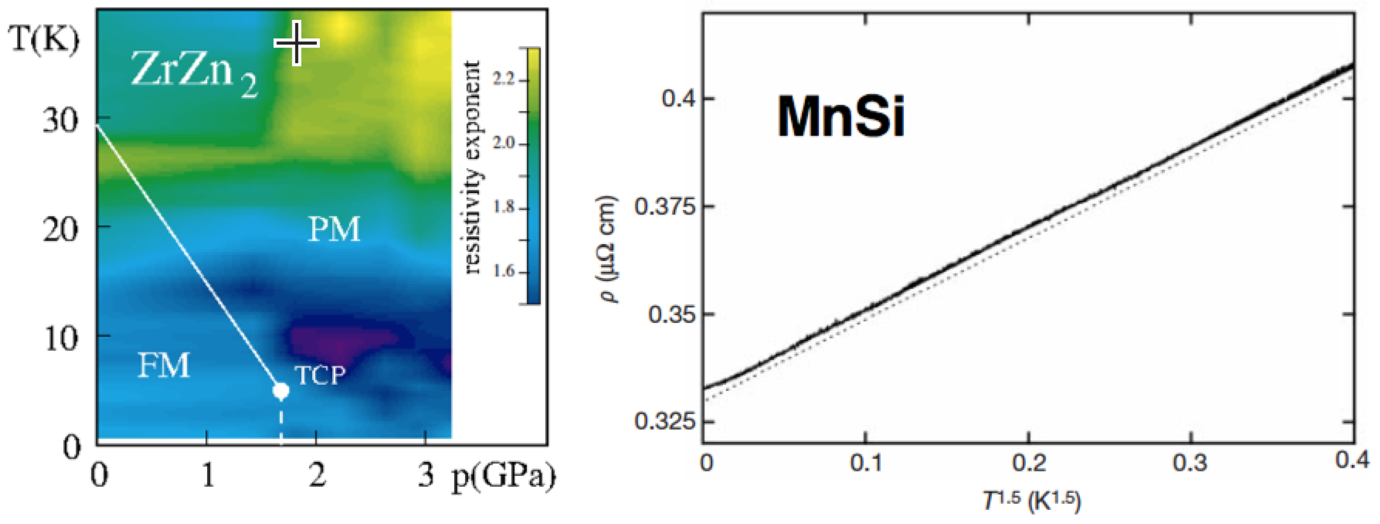
with the exponent $s<2$ is often referred to as “non-Fermi liquid” (NFL) (transport) behavior, although this designation requires some qualification as we discuss in Section 5. A prominent example is the linear T-dependence of the resistivity in the normal phase of hole-doped, high-T${}_c$ superconductors near optimal levels of doping [3,4]. Examples in other systems are provided by various ferromagnets with low Curie temperatures. Sato observed a behavior given by Equation (1) with $s\approx 1.50-1.65$ in Pd-doped Ni${}_3$Al [5]. A very similar behavior was found in pressure-tuned Ni${}_3$Al [6], as well as in pressure-tuned ZrZn${}_2$ [7]. Another example is provided by the helical magnet MnSi, which shows a very clean $s=3/2$ behavior in a temperature range from a few mK to several K [8]. The measured resistivities of ZrZn${}_2$ and MnSi are shown in Figure 1 as representative examples. We note that the anomalous transport behavior in ZrZn${}_2$ is observed in both the ordered and disordered phases, whereas in MnSi, it shows only in the disordered phase. In the helically-ordered phase of MnSi, $\delta \rho \propto T^2$ can be observed, albeit with a large prefactor ($A_2$), an observation we will come back to.

Surprisingly, this anomalous transport behavior is far from being completely understood, despite having been observed for many decades in many different materials. In this paper, we provide a pedagogical overview of this problem and the solutions that have been proposed.

2. Soft Modes as the Origin of Power Law Relaxation Rates

It is intuitively plausible that any power law behavior of relaxation rates, including those that determine transport coefficients, requires the scattering of conduction electrons by soft or massless excitations, i.e., excitations whose characteristic frequency vanishes in the limit of the vanishing wave number. A gapped excitation, whose frequency remains non-zero in this limit, will get frozen out at low temperatures compared to the gap and produce an exponentially small relaxation rate. This can be demonstrated explicitly by means of some very simple and general arguments.

As a very simple schematic example, consider non-interacting electrons described by the action $S_0[\overline{\psi },\psi ]$. $\overline{\psi }(x)$ and $\psi (x)$ are fermionic fields, $x\equiv (\overrightarrow{x},\tau )$ comprises the real-space position $\overrightarrow{x}$ and the imaginary-time variable $\tau$, and we suppress discrete degrees of freedom such as spin, band indices, etc., in our notation. Let the single-electron energy-momentum relation be ${ϵ}_{\overrightarrow{k}}$, and denote the chemical potential by $\mu$. The Fermi surface is then characterized by ${\xi }_{\overrightarrow{k}}\equiv {ϵ}_{\overrightarrow{k}}-\mu =0$. Consider a generalized electron density of $n(x)=\overline{\psi }(x)\psi (x)$ and its fluctuations ($\delta n(x)=n(x)-\langle n(x)\rangle$), and denote its Fourier transform by $n(k)$, with $k\equiv (\overrightarrow{k},{\omega }_n)$ being a 4-vector that comprises a wave vector ($\overrightarrow{k}$) and a fermionic Matsubara frequency (${\omega }_n$). Examples of $n(x)$ are the number density, the spin density, or any other moment of a general phase space density. In addition, let $\delta N(x)$ be a non-electronic density fluctuation that is governed by a Gaussian action,

$$S_{\mathrm{fluct}}\left[\delta N\right]=\frac{-1}{2}\int dxdy\delta N(x){\chi }^{-1}(x-y)\delta N(y),$$

(2)

with $\chi$ being the physical susceptibility that is appropriate for the $\delta N$ fluctuations and couples to the electronic density via a short-ranged interaction, potential (v):

$$S_{\mathrm{coup}}=\int dxdy\delta N(x)\delta ({\tau }_x-{\tau }_y)v(\overrightarrow{x}-\overrightarrow{y})\delta n(y).$$

(3)

An example of $\delta N$ is the ionic density fluctuations, in which case n is the electronic number density, v is the screened Coulomb interaction, and $S_{\mathrm{coup}}$ describes the electron–phonon coupling. If we integrate out the $\delta N$ fluctuations, we obtain an effective electronic action of

$$S_{\mathrm{eff}}[\overline{\psi },\psi ]=S_0[\overline{\psi },\psi ]+\frac{1}{2}{\int }_k\delta n(k)V(k)\delta n(-k),$$

(4a)

with an effective potential of $V(k)={\left(v(\overrightarrow{k})\right)}^2\chi (k)$. Since the potential (v) is short-ranged, we can, for the purpose of studying long-wavelength effects, replace this expression by

$$V(k)=C\chi (k)$$

(4b)

with $C=v^2(\overrightarrow{k}=0)$ being a coupling constant. The integration measures in Equations (2), (3) and (4a), respectively, are $\int dx\equiv {\int }_{V}d\overrightarrow{x}{\int }_0^{1/T}d\tau$ and ${\int }_k=(1/V){\sum }_{\overrightarrow{k}}T{\sum }_{{\omega }_n}$, with V being the system volume. We use units such as the Boltzmann constant ($k_{\mathrm{B}}=1$).

The effective electron–electron interactions described by V can be interpreted as an exchange of $\delta N$ fluctuations by the electrons. This leads to an electron self energy that is given, by Hartree–Fock approximation, by

$$\Sigma (p)={\int }_{k}V(k)G(p-k).$$

(5)

The single-particle relaxation rate ($1/{\tau }_{\mathrm{sp}}$), i.e., the inverse quasiparticle lifetime due to the effective interaction, averaged over the Fermi surface, is given by

$$\begin{array}{ccc}\hfill \frac{1}{2{\tau }_{\mathrm{sp}}}& =& \frac{-1}{N_{\mathrm{F}}V}\sum _{\overrightarrow{p}}\delta ({\xi }_{\overrightarrow{p}}){\Sigma }^{″}(\overrightarrow{p},0)\hfill \\ & =& 2N_{\mathrm{F}}{\int }_{-\infty }^{\infty }du{\overline{V}}^{″}(u)\frac{1}{sinh(u/T).}\hfill \end{array}$$

(6)

Here, $N_{\mathrm{F}}$ is the electronic density of the states at the Fermi surface, ${\Sigma }^{″}(\overrightarrow{p},\omega )=\mathrm{Im}\Sigma (\overrightarrow{p},i{\omega }_n\to \omega +i0)$ is the spectrum of the self energy, and

$${\overline{V}}^{″}(u)=\frac{1}{{(N_{\mathrm{F}}V)}^2}\sum _{\overrightarrow{k},\overrightarrow{p}}\delta ({\xi }_{\overrightarrow{k}})\delta ({\xi }_{\overrightarrow{p}})V^{″}(\overrightarrow{k}-\overrightarrow{p},u)$$

(7)

is the spectrum of the effective potential averaged over the Fermi surface. For simplicity, we ignore the splitting of the Fermi surface in magnets for the time being. We add this feature and several important others in Section 4.

2.1. Power Law Relaxation Rates from the Exchange of Particles

To specify the effective potential (V), consider a particle-like excitation with a wave-number dependent resonance frequency of ${\omega }_0(\overrightarrow{k}\to 0)=c{|\overrightarrow{k}|}^n$, in which case, the spectrum of the susceptibility ($\chi$) has the form

$${\chi }^{″}(\overrightarrow{k},u)\propto {|u|}^m\mathrm{sgn}(u)\delta (u^2-{\omega }_0^2(\overrightarrow{k})).$$

(8)

Here, c is a stiffness coefficient, and we ignore a prefactor that we absorb into the coupling constant (C), and we neglect any damping of the excitation. The values of exponents n and m depend on the nature of the particles. Examples are shown below.

By performing the wave-number integrals in Equation (7), we find

$${\overline{V}}^{″}(u)\propto {|u|}^{m+(d-1-2n)/n}\mathrm{sgn}(u).$$

(9)

Via Equation (6), this leads to

$$1/{\tau }_{\mathrm{sp}}\propto T^{m+(d-1-n)/n}$$

(10)

with d being the spatial dimensionality.

These simple considerations illustrate a basic point: the power law behavior of $1/{\tau }_{\mathrm{sp}}$ hinges on the resonance frequency ${\omega }_0$ by scaling as a power of $|\overrightarrow{k}|$ for $\overrightarrow{k}\to 0$. This is the defining property of a mode that is soft, gapless, or massless.

As a well-known example, consider longitudinal phonons. In this case, $\delta n$ and $\delta N$ are the electronic and ionic number density fluctuations, respectively, and v is a screened Coulomb interaction. The susceptibility ($\chi$) has the same form as in a classical fluid and is characterized by $m=2$ and $n=1$ [10]. We thus have $1/{\tau }_{\mathrm{sp}}\propto T^d$. In $d=3$, this is the well-known $T^3$ law for the single-particle relaxation rate due to phonons [11].

We note that we have made several simplifying assumptions so far, in addition to the assumption of the single Fermi surface mentioned above. First, we have considered only the single-particle relaxation rate, rather than the more complicated transport rate, $1/{\tau }_{\mathrm{tr}}$, which determines the electrical resistivity. The single-particle rate does, however, have the same T-dependence as the thermal resistivity, at least at the level of the Boltzmann equation [1]. Second, we have assumed an isotropic resonance frequency that depends only on the magnitude of the wave vector. Third, we have ignored the effects of quenched disorder, which is always present in real materials (sometimes only very weakly). Relaxing these constraints is important in order to understand the experimental results that we are interested in; we will discuss this in Section 4.

2.2. Power Law Relaxation Rates from the Exchange of Unparticles

Another possibility is the exchange of fluctuations that have been dubbed ‘unparticles’ in a particle physics context [12]. They are characterized by a continuous spectrum that is scale invariant but lacks the resonance peak characteristic of particles:

$${\chi }^{″}(\overrightarrow{k},u)\propto u^m/{|\overrightarrow{k}|}^n.$$

(11)

Spectra of this type are actually very familiar from condensed matter physics; the most common example is the Lindhard function [13]. The wave vector integrals in Equation (7) then simply lead to a prefactor, and the single particle and transport rates are the same, except for having a prefactor of $O(1)$, $1/{\tau }_{\mathrm{sp}}\approx 1/{\tau }_{\mathrm{tr}}\equiv 1/\tau$. The temperature dependence of either relaxation rate is determined by exponent m only, and we have

$$1/\tau \propto T^{m+1}.$$

(12)

An obvious example is the case of Coulomb scattering. In this case, $\delta N$ and $\delta n$ both represent electronic number density fluctuations that interact via a screened Coulomb interaction. ${\chi }^{″}$ then is the spectrum of the Lindhard function, and hence, $m=n=1$, which leads to $1/\tau \propto T^2$. We note that at the level of quantum electrodynamics, the objects exchanged by the electrons in this example are, of course, particles, namely, virtual photons. However, at the level of an effective low energy theory where the microscopic details have been integrated out, the effects of this exchange manifest themselves in the form of a continuous spectrum, namely, the dynamically screened Coulomb interaction.

For later reference, we restore the prefactors, which leads to a familiar result for the Coulomb scattering rate,

$$1/\tau =\pi T^2/2{ϵ}_{\mathrm{F}},$$

(13)

with ${ϵ}_{\mathrm{F}}$ being the Fermi energy. The above derivation is similar in spirit to the one presented in Reference [14]. It is remarkable that the argument of interacting density fluctuations still works if the $\delta N$ fluctuation that interacts with the electronic $\delta n$ fluctuation is itself an electronic density fluctuation created by all the other electrons. This aspect was stressed in Reference [15].

3. Experimental Results

To classify experimental results that show anomalous transport behavior, it is crucial to distinguish between two different cases. In the first case, the anomalous behavior is observed only in a narrow region of the phase diagram, usually in the vicinity of a known or suspected critical point. Its observation thus requires fine tuning. An example is the $T^{3/2}$ resistivity combined with a logarithmic T-dependence of the specific heat coefficient observed near a probable quantum critical point in NbFe${}_2$ [16]. In the second case, the anomalous behavior is generic in the sense that it is observed in large regions of the phase diagram. This distinction is crucial, since critical points necessarily lead to critical fluctuations that can serve as the scale invariant excitations that underlie the mechanism discussed in Section 2. Another important distinction is between clean systems that contain no or very little quenched disorder and disordered ones. This is because quenched disorder leads to diffusive electron dynamics that can lead to anomalous transport behavior via well-known mechanisms [17,18]. The anomalous transport behavior that is hardest to understand thus occurs in systems that are clean, as evidenced by a small residual electric resistivity (${\rho }_0$) or a large mean-free path and show generic anomalous behavior that does not require fine tuning.

Two materials that fall into the latter category are the ferromagnet ZrZn${}_2$, and the helimagnet MnSi. The cleanest samples for either system have ${\rho }_0\approx 0.3\mathsf{\mu }\Omega$cm, and the transition from the magnetic to the non-magnetic phase can be triggered by applying hydrostatic pressure. The magnetic quantum phase transitions have been well established to be first-order [19,20], so critical fluctuations are not a viable candidate for explaining the observed transport anomalies (see Reference [21] and references therein for a review of the magnetic properties of these materials).

The phase diagram of ZrZn${}_2$ is shown in Figure 1. The resistivity exponent s, determined by the slope of a log-log plot of the electrical resistivity, is less than 2 in a large part of the phase diagram, ranging from ambient pressure to twice the critical pressure, and from the lowest temperatures achievable to about 20 K. The smallest exponent, $s\approx 1.5$, was found in a temperature region around 10 K in the paramagnetic phase [7]. Data at ambient pressure have been fitted to Equation (1) with $s=5/3$ for samples with residual resistivities between $0.3\mathsf{\mu }\Omega$cm and $6.4\mathsf{\mu }\Omega$cm, while a magnetic field of 9T restores $T^2$ behavior [22]. The respective prefactors are $A_{5/3}\approx 0.021\mathsf{\mu }\Omega$cm/K${}^{5/3}$ and $A_2\approx 0.003\mathsf{\mu }\Omega$cm/K${}^2$. We discuss interpretations of this behavior in Section 4 and Section 5, where we show that an equally good fit of the data is obtained by superpositions of $s=3/2$ and $s=2$.

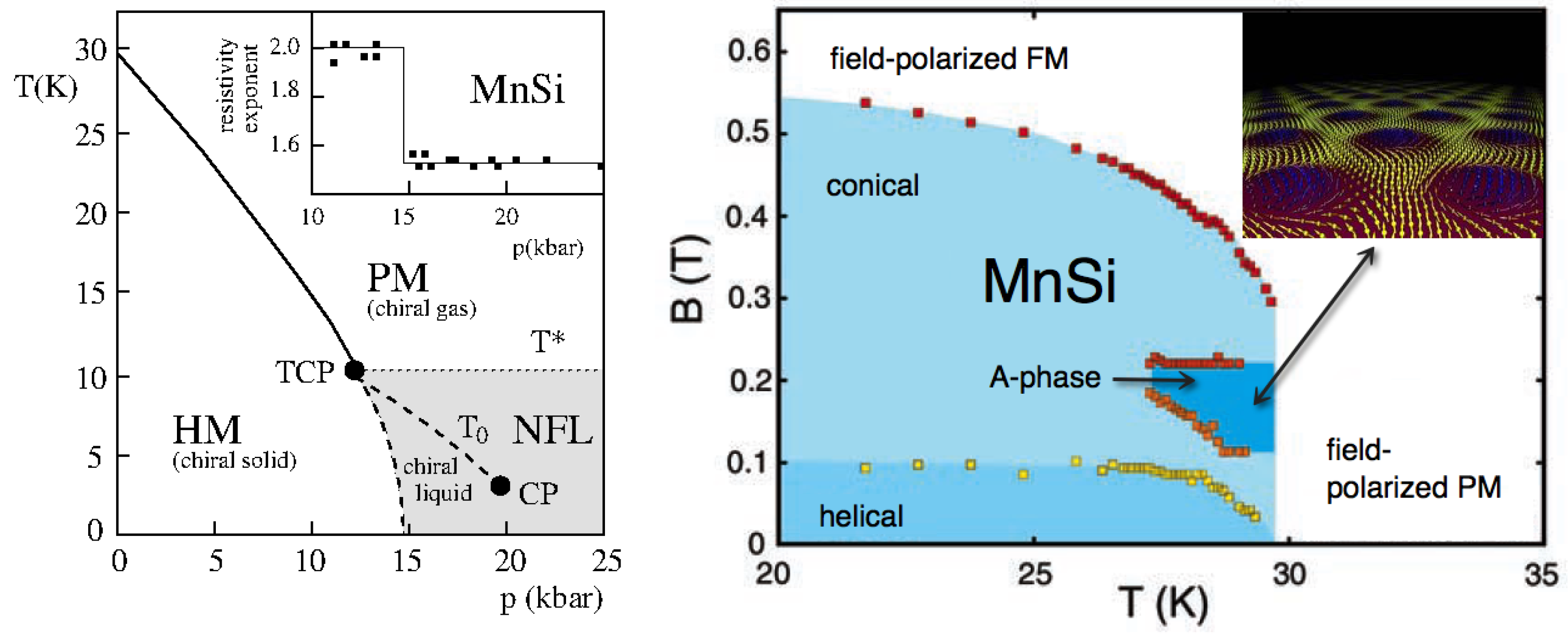
MnSi is a helimagnet with a rather long helical pitch wavelength of about 180 Å [23]. Hydrostatic pressure destroys the helical order [20] and drives the system into a phase with no long-range magnetic order. There is, however, evidence for strong fluctuations in the non-magnetic phase [24]. The phase diagram in the temperature–pressure plane is shown in the left panel of Figure 2. The magnetic phase transition at low temperatures is first-order, as is generically the case in clean metallic ferromagnets and long-wavelength helimagnets (for a review of the magnetic properties, see Reference [21]). Throughout the non-magnetic phase, from a critical pressure of $p_c\approx 15$ kbar to about 50 kbar, and over a temperature range from a few mK to almost 10 K, the electrical resistivity displays a $T^{3/2}$ behavior with a prefactor ranging from $A_{3/2}\approx 0.1\mathsf{\mu }\Omega$cm/K${}^{3/2}$ at high pressure to $0.22\mathsf{\mu }\Omega$cm/K${}^{3/2}$ near the critical pressure [8,25] (see Figure 1 and Figure 2). In the helical phase, the electrical resistivity shows a $T^2$ behavior with a prefactor of $A_2\approx 0.03\mathsf{\mu }\Omega$cm/K${}^2$ at ambient pressure that rises, first gradually, and eventually sharply, to $A_2\approx 0.12\mathsf{\mu }\Omega$cm/K${}^2$ as the critical pressure is approached from below [25]. We note that these prefactors are surprisingly large. They are larger by a factor of 10 compared to their counterparts in ZrZn${}_2$, and larger by many orders of magnitude compared to the Coulomb scattering contribution given by the Drude formula in conjunction with the scattering rate in Equation (13). The $T^2$ behavior in the helical phase is thus as anomalous as the $T^{3/2}$ behavior in the disordered phase, even though the exponent value happens to coincide with the one that is characteristic of ordinary Fermi liquid behavior.

In a magnetic field, MnSi has a phase known as the A-phase that consists of a skyrmionic spin texture, with the cores of the skyrmions forming a hexagonal lattice of columns in the material [27] (see the right panel in Figure 2). The $T^{3/2}$ behavior of the resistivity in the paramagnetic phase persists in a non-zero field up to the crossover to the field-polarized ferromagnetic region, and neutron scattering has provided evidence for strong fluctuations in the paramagnetic phase [24].

Neither in the case of ZrZn${}_2$, nor in that of MnSi is there any reason to believe that either critical fluctuations or diffusive electron dynamics lead to the observed anomalous transport behavior. The explanation thus must lie in generic excitations that are extraneous to the conduction electrons. We discuss proposals along these lines in Section 4.

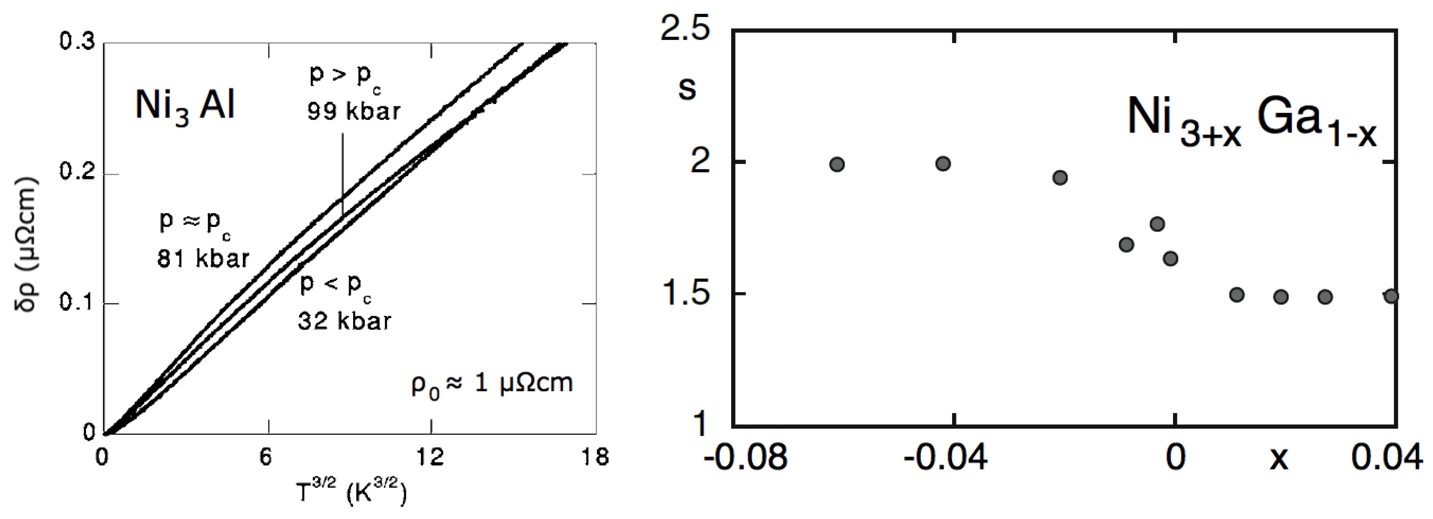
Another example of generic anomalous transport behavior in quantum magnets is provided by the isostructural compounds Ni${}_3$Al and Ni${}_3$Ga, which can be prepared with various Ni concentrations around the stoichiometric value. Ni${}_3$Al has a ferromagnetic order below 15–41 K, depending on the exact composition, and a ferromagnetic-to-paramagnetic quantum phase transition (QPT) can be triggered by means of hydrostatic pressure (see References [21,25] and references therein). The transition is suspected to be first-order [6,25], and stoichiometric samples have residual resistivities of ${\rho }_0\approx 1\mathsf{\mu }\Omega$cm. The resistivity exponent is $s\gtrsim 1.5$ on either side of the transition (see Figure 3), and the prefactor is $A_s\approx 0.01\mathsf{\mu }\Omega$cm/K${}^s$ [25]. Similar behavior is observed in Ni${}_{1-x}$Pd${}_x$)${}_3$Al, which undergoes a ferromagnetic QPT at $x\approx 0.095$ [5]. This transport behavior is very similar to that observed in ZrZn${}_2$. Stoichiometric Ni${}_3$Ga is paramagnetic and remains so for Ni-poor compositions, but it has a ferromagnetic ground state for Ni-rich compositions. In ferromagnetic samples, $s\approx 1.5$ with a prefactor of $A_{3/2}\approx 0.04\mathsf{\mu }\Omega$cm/K${}^{3/2}$, whereas $s=2$ in the paramagnetic samples with $A_2\approx 0.001\mathsf{\mu }\Omega$cm/K${}^2$ (see Reference [25] and references therein). This situation is the reverse of the one in MnSi, where $s=2$ in the magnetically ordered phase and $s=1.5$ in the disordered phase.

4. Theoretical Explanations

As we have seen in Section 2, any explanation of the generic transport anomalies observed in various quantum magnets must involve the scattering of electrons by soft generic excitations. In magnetically ordered phases, obvious candidates are the Goldstone modes that result from the magnetic order. In phases without long-range magnetic order, there are two possibilities. Strong fluctuations that are remnants of the long-range order may provide scattering mechanisms that can lead to generic transport anomalies. Candidates for such fluctuations have been observed in the non-magnetic phase of MnSi [24] and have been discussed as a possible origin of the observed $T^{3/2}$ behavior [30]. Alternatively, weak quenched disorder may provide droplets of the ordered phase within the disordered one (and vice versa) [31]. This explains the widespread observation of phase separation away from the coexistence curve of a first-order phase transition, and it also provides a way for scattering mechanisms that are germane to the magnetic phase to persist in parts of the disordered phase. We discuss these mechanisms in more detail later in this section and also in Section 5.

For ferromagnets in the ordered phase, the magnon contribution to the resistivity was considered early on and was found to produce a $T^2$ behavior [32,33], in agreement with experimental results on Fe, Co, and Ni [34]. Later work confirmed this, and also considered scattering by the continuum of Stoner excitations (another example of the ‘unparticles’ mentioned in Section 2) [35,36]. $T^2$ behavior is valid only above a characteristic temperature that is related to the exchange splitting [37], as we explain explicitly below. The behavior of both the electric and thermal resistivities in various temperature regimes was discussed in Reference [15]. For helimagnets, the Goldstone modes and their contribution to the scattering rates were derived in References [38,39,40,41]. Recently, electron scattering from Goldstone modes in both ferromagnets and helimagnets has been reconsidered, and several new mechanisms for anomalous transport behavior have been discussed [9]. In this section, we give a summary of the current state of the theory. We focus on three mechanisms that yield a resistivity exponent of $s=3/2$ in some temperature regime (for more complete results see Reference [9]). For completeness, and to clarify some common misconceptions, we also briefly discuss the effects of non-generic critical fluctuations and the extent to which they exist.

4.1. Scattering by Magnetic Goldstone Modes

As mentioned in Section 2, the basic considerations presented need to be generalized and refined in several ways in order to be applicable to magnetic materials. We start with a discussion of clean systems, and then consider the effects of weak disorder.

4.1.1. Clean Systems

In the ordered phase of both ferromagnets and helimagnets, the effective local magnetic field seen by the conduction electrons leads to an exchange splitting ($\lambda$) of the Fermi surface. We thus need to distinguish between intraband scattering, where a magnon is exchanged between electrons in the same sub-band of the exchange-split Fermi surface, and interband scattering, where the exchange is between electrons in different sub-bands. At asymptotically low temperatures in clean systems, the latter will always lead to exponentially small rates, as the scattering processes gets frozen out for small temperatures compared to the exchange splitting. However, they can provide the leading contribution to scattering in a pre-asymptotic temperature window whose lower limit can be rather low, and thus needs to be considered. Furthermore, weak quenched disorder eliminates the exponential suppression, as we will see. In ferromagnets, the magnons do not couple electrons in the same sub-band, and thus, interband scattering is the only mechanism available. The effective potential for interband scattering is given by Equation (7), but with shifted arguments of the $\delta$-functions that reflect the fact that the electrons with a wave vector of $\overrightarrow{k}$ live on a different Fermi surface than those with a wave vector of $\overrightarrow{p}$. The coupling constant (C) is given by the square of the exchange interaction (${\mathsf{\Gamma }}_t$), and the resulting expression for the single-particle interband scattering rate is

$$\frac{1}{{\tau }_{\mathrm{sp}}}\propto N_{\mathrm{F}}{\mathsf{\Gamma }}_t^2{\int }_{-\infty }^{\infty }du\frac{1}{sinh(u/T)}\frac{1}{N_{\mathrm{F}}^2{V}^2}\sum _{\overrightarrow{k},\overrightarrow{p}}\delta ({\xi }_{\overrightarrow{k}+\overrightarrow{p}}-\lambda )\delta ({\xi }_{\overrightarrow{p}}+\lambda ){\chi }^{″}(\overrightarrow{k},u).$$

(14)

The transport rate is given by the same expression with an additional factor of ${\overrightarrow{k}}^2/k_{\mathrm{F}}^2$ in the integrand, with $k_{\mathrm{F}}$ being the Fermi wave number. This is known as the backscattering factor that suppresses large-angle scattering [1]. For the transport interband scattering rate, we thus have

$$\frac{1}{{\tau }_{\mathrm{tr}}}\propto N_{\mathrm{F}}{\mathsf{\Gamma }}_t^2{\int }_{-\infty }^{\infty }du\frac{1}{sinh(u/T)}\frac{1}{N_{\mathrm{F}}^2{V}^2}\sum _{\overrightarrow{k},\overrightarrow{p}}({\overrightarrow{k}}^2/k_{\mathrm{F}}^2)\delta ({\xi }_{\overrightarrow{k}+\overrightarrow{p}}-\lambda )\delta ({\xi }_{\overrightarrow{p}}+\lambda ){\chi }^{″}(\overrightarrow{k},u).$$

(15)

4.1.2. Systems with Weak Disorder

Quenched disorder, however weak, is present in all real materials and leads to a non-zero scattering rate of $1/{\tau }_0$, even at $T=0$, and a corresponding residual resistivity (${\rho }_0$). The cleanest samples of the magnetic systems discussed here have residual resistivities of a few tenths of a $\mathsf{\mu }\Omega$ cm. While being very clean by the standards of these compounds, these values are large compared to the residual resistivities of many non-magnetic metals (e.g., the residual resistivity of commercial Cu wire is less than $1$n$\Omega$ cm). This motivates the consideration of disorder in the ballistic or weak disorder regimes [42], which, in magnets, is characterized by the condition $\lambda {\tau }_0\gg 1$ [41]. A rigorous treatment requires elaborate diagrammatic calculations, but the net effect can be described by using simple heuristic arguments [9].

Next, we consider the expression for the clean single particle rate in Equation (14). Performing the wave number convolution integral yields

$$\frac{1}{N_{\mathrm{F}}V}\sum _{\overrightarrow{p}}\delta ({\xi }_{\overrightarrow{k}+\overrightarrow{p}}-\lambda )\delta ({\xi }_{\overrightarrow{p}}+\lambda )\propto {\int }_{-1}^{1}d\eta \delta (k{v}_{\mathrm{F}}\eta -2\lambda )=\frac{1}{v_{\mathrm{F}}|\overrightarrow{k}|}\mathsf{\Theta }(|\overrightarrow{k}|-2\lambda /v_{\mathrm{F}})$$

(16)

where $v_{\mathrm{F}}$ is the Fermi velocity. The step function leads to exponential suppression of the rates at the asymptotically low temperatures mentioned above [15,37]. In a weak disorder, the $\delta$-function is replaced with a Lorentzian, and in the limit $v_{\mathrm{F}}|\overrightarrow{k}|/\lambda \ll 1$, $\lambda {\tau }_0\gg 1$ the step function gets replaced by

$$\frac{1}{v_{\mathrm{F}}|\overrightarrow{k}|}\mathsf{\Theta }(|\overrightarrow{k}|-2\lambda /v_{\mathrm{F}})={\int }_{-1}^{1}d\eta \delta (k{v}_{\mathrm{F}}\eta -2\lambda )\to {\int }_{-1}^{1}d\eta \frac{1/{\tau }_0}{(v_{\mathrm{F}}|\overrightarrow{k}{|\eta -2\lambda )}^2+1/{\tau }_0^2}\approx \frac{1}{{\lambda }^2{\tau }_0}$$

(17)

The disorder thus eliminates the lower cutoff for the $\overrightarrow{k}$-integral and leads to an extra factor of $v_{\mathrm{F}}|\overrightarrow{k}|/{\lambda }^2{\tau }_0$ in the integrand. Since $\overrightarrow{k}$ scales as a positive power of the temperature, this implies that the power law T-dependence of the single particle rate is weaker than in the corresponding clean system, but extends to a temperature of zero.

In the case of the transport rate, the same arguments apply, but, in addition, the disorder eliminates the backscattering factor, since it leads to more isotropic scattering. The effective extra factor in the integrand is thus $({ϵ}_{\mathrm{F}}/{\lambda }^2{\tau }_0)k_{\mathrm{F}}/|\overrightarrow{k}|$, and the disorder strengthens the T-dependence of the rate, in addition to eliminating the exponential suppression at asymptotically low T values. The single particle rate and the transport rate are thus qualitatively the same and are given by

$$\frac{1}{{\tau }_{\mathrm{sp}}}\propto \frac{1}{{\tau }_{\mathrm{tr}}}\propto \frac{N_{\mathrm{F}}{\mathsf{\Gamma }}_t^2}{{\lambda }^2{\tau }_0}{\int }_{-\infty }^{\infty }du\frac{1}{sinh(u/T)}\frac{1}{N_{\mathrm{F}}V}\sum _{\overrightarrow{k}}{\chi }^{″}(\overrightarrow{k},u).$$

(18)

$1/{\tau }_{\mathrm{tr}}$ and $1/{\tau }_{\mathrm{sp}}$ determine the electrical and thermal resistivities via the Drude formula:

$$\rho =m_{\mathrm{e}}/n_{\mathrm{e}}{e}^2\tau ,$$

(19)

where e, $m_{\mathrm{e}}$, and $n_{\mathrm{e}}$ represents the electron charge, mass, and density, respectively.

4.2. Application to Quantum Ferromagnets

Now, consider the scattering of electrons by magnons in ferromagnets. The relevant resonance frequency (${\omega }_0$ in Section 2) is

$${\omega }_{\mathrm{FM}}(\overrightarrow{k}\to 0)=D{\overrightarrow{k}}^2$$

(20)

with D being the spin stiffness coefficient, and the corresponding susceptibility is, apart from a numerical prefactor [10],

$${\chi }_{\mathrm{FM}}(\overrightarrow{k},i\Omega )\propto \frac{m_{0}D{\overrightarrow{k}}^2}{{\omega }_{\mathrm{FM}}{(\overrightarrow{k})}^2-{(i\Omega )}^2}.$$

(21)

$m_0$ is the magnetization scale that determines the exchange splitting ($\lambda$) via $\lambda ={\mathsf{\Gamma }}_t{m}_0$. Two other relevant energy scales represent the largest amount of energy that can be carried by a magnon (i.e., the magnetic equivalent of the Debye temperature),

$$T_1=D{k}_{\mathrm{F}}^2,$$

(22)

and the smallest amount of energy that can be transferred by means of magnon exchange,

$$T_0=D{k}_0^2\approx T_1{(\lambda /{ϵ}_{\mathrm{F}})}^2,$$

(23)

where $k_0=\lambda /v_{\mathrm{F}}$.

For clean ferromagnets, Equations (14) and (15) yield the results shown in References [15,35,37], namely, $TlnT$and $T^2$ behavior for $1/{\tau }_{\mathrm{sp}}$ and $1/{\tau }_{\mathrm{tr}}$, respectively, for $T_0<T<T_1$, and exponentially small rates for $T<T_0$. In the presence of ballistic quenched disorder, Equation (18) leads to both rates scaling as $T^{3/2}$, which results in the resistivity contribution

$$\delta {\rho }_{\mathrm{FM}}=A_{3/2}^{\mathrm{FM}}{T}^{3/2},$$

(24a)

with a prefactor of

$$A_{3/2}^{\mathrm{FM}}={\gamma }_1{\rho }_0/T_1\sqrt{T_0},$$

(24b)

where ${\gamma }_1$ is a numerical prefactor. Since the single particle rate has the same T-dependence as the transport rate, this result also holds for the thermal resistivity—only the numerical prefactor is different. It is valid for $T_{\mathrm{ball}}\ll T\lesssim T_0$, with

$$T_{\mathrm{ball}}=T_1/{({ϵ}_{\mathrm{F}}{\tau }_0)}^2.$$

(25)

The lower limit on the temperature window is dictated by the constraints on the ballistic disorder regime [9]. For lower temperatures, the electron dynamics are diffusive.

The appropriate parameter values for ZrZn${}_2$ were estimated in Reference [9]. The result was a prefactor of $A_{3/2}^{\mathrm{FM}}\approx 0.01\mathsf{\mu }\Omega$cm/K${}^{3/2}$, which is very close to what is observed in this material (see the discussion in Section 3 and Section 5). In order for this mechanism to explain the anomalous transport behavior on either side of the first-order QPT, the droplet formation discussed in Reference [31] is crucial.

4.3. Application to Quantum Helimagnets

In helimagnets, there are two different soft modes that are candidates for explaining anomalous transport behavior. One is the helimagnons, which are the Goldstone modes of the spontaneously broken symmetry that is present in the helically-ordered phase [38]. The other is fluctuations of the columnar skyrmion structure that is observed, e.g., in the A-phase of MnSi (see Figure 2 and Reference [27]). Columnar fluctuations are familiar from the theory of liquid crystals [43] and were studied in the context of helimagnets in References [30] and [44].

4.3.1. Scattering by Columnar Fluctuations in the Skyrmionic Phases

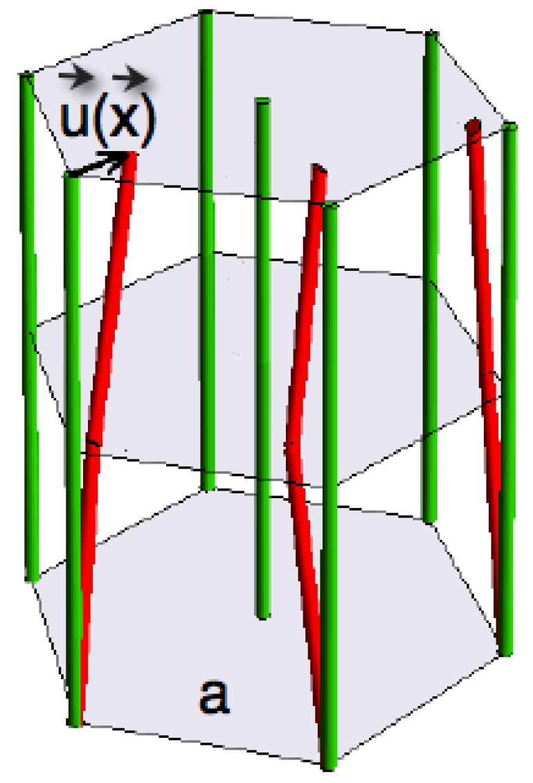
Consider a hexagonal lattice of columns in the z-direction that fluctuate about their equilibrium positions, as shown in Figure 4. Such fluctuations have an anisotropic dispersion relation, with the resonance frequency scaling linearly with the wave number for the wave vectors (${\overrightarrow{k}}_{\perp }$) perpendicular to the columns, and quadratically with the wave number for wave vectors in the direction of the columns [43]. If the columnar structure is due to skyrmions comprising a superposition of three helices with a pitch wave number of q, as proposed in Reference [27], then the resonance frequency is [9,45]

$${\omega }_{\mathrm{sky}}(\overrightarrow{k})=\left\{\begin{array}{ccc}D\sqrt{k_z^4+{\overrightarrow{k}}_{\perp }^2{q}^2}\hfill & \mathrm{for}\hfill & D{q}^4/k_{\mathrm{F}}^2\lesssim {\omega }_{\mathrm{sky}}\lesssim D{q}^2\hfill \\ D(k_{\mathrm{F}}^2/q^2)(k_z^4/q^2+{\overrightarrow{k}}_{\perp }^2)\hfill & \mathrm{for}\hfill & {\omega }_{\mathrm{sky}}\lesssim D{q}^4/k_{\mathrm{F}}^2.\hfill \end{array}\right.$$

(26)

For ${\omega }_{\mathrm{sky}}\gtrsim D{q}^2$, the behavior crosses over to the ferromagnetic one given by Equation (20). The corresponding susceptibility is

$${\chi }_{\mathrm{sky}}(\overrightarrow{k},i\Omega )\propto \frac{m_0}{{\omega }_{\mathrm{sky}}^2(\overrightarrow{k})-{(i\Omega )}^2}\left\{\begin{array}{ccc}D{q}^2\hfill & \mathrm{for}\hfill & {\omega }_{\mathrm{sky}}\gtrsim D{q}^4/k_{\mathrm{F}}^2\hfill \\ {(k_{\mathrm{F}}/q)}^2{\omega }_{\mathrm{sky}}(\overrightarrow{k})\hfill & \mathrm{for}\hfill & {\omega }_{\mathrm{sky}}\lesssim D{q}^4/k_{\mathrm{F}}^2.\hfill \end{array}\right.$$

(27)

In the presence of ballistic disorder, the behavior of the mode in the upper frequency range leads, in conjunction with Equation (18), to qualitatively equal results for the electrical and thermal resistivities as in the ferromagnetic case:

$$\delta {\rho }_{\mathrm{sky}}=A_{3/2}^{\mathrm{sky}}{T}^{3/2}$$

(28a)

with the prefactor

$$A_{3/2}^{\mathrm{sky}}={\gamma }_2{\rho }_0/T_1\sqrt{T_0},$$

(28b)

where ${\gamma }_2$ is another numerical factor. This is valid for Max($T_{\mathrm{ball}},T_q{q}^2/k_{\mathrm{F}}^2)\lesssim T\lesssim T_q$, with

$$T_q=D{q}^2$$

(29)

being another energy scale—this one is relevant for helimagnets. Since the behavior for $T\gtrsim T_q$ crosses over to ferromagnetic, which is the same, except for the numerical prefactor, the effective upper limit of the region of validity is the greater value of $T_0$ and $T_q$.

For temperatures lower than $T_q{(q/k_{\mathrm{F}})}^2$, the lower frequency regime in Equations (26) and (27) is relevant, and the T-dependence of the resistivity crosses over to a $T^{5/4}$ behavior. However, for helimagnets with a small $q/k_{\mathrm{F}}$, this crossover temperature is extremely low and may not be larger than $T_{\mathrm{ball}}$, so this behavior may not be observable. For instance, an estimate for MnSi yields [9] $T_q\approx 250$mK, $T_{\mathrm{ball}}\approx 1$ mK. With $q/k_{\mathrm{F}}\approx 0.03$ [23], this yields a crossover temperature of about 0.2 mK, which is lower than $T_{\mathrm{ball}}$ and hence, is not observable.

Using parameter values that are appropriate for MnSi, an estimate of the prefactor shows that it is within a factor of 5 within what is observed in the non-magnetic phase of MnSi can be determined [9]. In order for this mechanism to be operative in that phase, strong columnar fluctuations must exist. There is experimental evidence for this to be the case [24]. A theoretical analysis of the possible nature of this phase was given in Reference [26].

4.3.2. Scattering by Helimagnons

A third mechanism for $T^{3/2}$ behavior of the electrical resistivity is provided by scattering of electrons by helimagnons, the Goldstone modes of helical order, in clean helimagnets. The dispersion relation and the susceptibility for the helimagnons are [38]

$${\omega }_{\mathrm{HM}}(\overrightarrow{k})=D\sqrt{q^2{k}_z^2+{\overrightarrow{k}}_{\perp }^4}$$

(30)

and

$${\chi }_{\mathrm{HM}}(\overrightarrow{k},i\Omega )\propto \frac{m_{0}D{q}^2}{{\omega }_{\mathrm{HM}}^2(\overrightarrow{k})-{(i\Omega )}^2}.$$

(31)

Here, q is the modulus of the helical pitch wave vector, which we again take to point in the z-direction. This is valid for ${\omega }_{\mathrm{HM}}\lesssim D{q}^2$—for larger wave numbers, the behavior crosses over to the ferromagnetic one. We note that the numerator of the susceptibility is independent of the wave number, whereas in the ferromagnet, it is proportional to ${\overrightarrow{k}}^2$. As a result, the helimagnon’s susceptibility is softer than the ferromagnon’s, even though the Goldstone mode is stiffer in the helimagnet than in the ferromagnet.

Equation (15) now yields a contribution to the electrical resistivity that is given by [9]

$$\delta {\rho }_{\mathrm{HM}}=A_{3/2}^{\mathrm{HM}}{T}^{3/2}$$

(32a)

with

$$A_{3/2}^{\mathrm{HM}}={\rho }_{\lambda }{\gamma }_{3}q/k_{\mathrm{F}}{T}_1^{3/2}.$$

(32b)

Here, ${\rho }_{\lambda }=\lambda m_{\mathrm{e}}/n_{\mathrm{e}}{e}^2$ is a resistivity scale, and ${\gamma }_3$ is another numerical factor. This result is valid for $T_0\lesssim T\lesssim T_q$, provided this window exists; for $T\lesssim T_0$, the rate is exponentially suppressed. In MnSi, the window does not exist, since $T_q<T_0$ [9].

In the presence of ballistic disorder, Equations (30) and (31) in conjunction with Equation (18) yield a stronger T-dependence, namely, $\delta {\rho }_{\mathrm{HM}}\propto TlnT$. At sufficiently low temperatures, the observed $T^2$ behavior of unknown origin is predicted to cross over to this behavior (see Reference [9] and the discussion in Section 5 below).

4.4. Scattering by Critical Fluctuations

By now, it has been well established, both theoretically and experimentally, that the QPT in clean metallic ferromagnets is generically first-order [21]. However, historically, it was believed that the transition was second-order and hence, accompanied by critical fluctuations [46]. We briefly discuss the influence of these fluctuations on the resistivity for two reasons: (1) the transition can be weakly first-order in some materials, and critical fluctuations may be observable in a pre-asymptotic regime, and (2) early work concerning the critical behavior has influenced the analysis of experiments, even in cases where later studies found a clear first-order transition.

Mathon [47] found the resistivity exponent $s=5/3$ due to ferromagnetic quantum critical fluctuations even before Hertz [46] developed a renormalization group treatment of QPTs. The same result was obtained by Millis [48] with renormalization group techniques (for a discussion of how this fits into a general scaling description of QPTs see Reference [49]). The exponent $5/3\approx 1.67$ can be experimentally hard to distinguish from 3/2, especially if there are various competing power law contributions to the resistivity that hold only in temperature windows of limited sizes (see Figure 5 and the related discussion). Furthermore, the critical fluctuations, if any, will be present only in a rather limited region of the phase diagram and cannot explain observations of anomalous transport behavior far from any phase transition. Still, they may well contribute to parts of the phase diagram in materials where the QPT is weakly first-order.

Sufficiently strong quenched disorder (strong enough to lead to diffusive electron dynamics) changes the nature of the ferromagnetic QPT from first- to second-order. This was predicted theoretically [50,51,52] and recently observed in Fe-doped MnSi [53]. The asymptotic critical behavior at this quantum critical point is unusual and very hard to observe [51], but in a pre-asymptotic region, an effective power-law behavior with the exponent $s=3/11$ has been predicted [49,52].

5. Discussion

We conclude by discussing various additional points and open problems.

5.1. Fermi Liquids and Non-Fermi Liquids

The anomalous transport behavior discussed in this paper is often referred to as non-Fermi liquid (NFL) behavior. However, this term has multiple meanings. Originally devised to describe the low-temperature behavior of fermions with a short-ranged interactions, such as He${}^3$ [54,55,56], Landau’s Fermi liquid theory was generalized to electrons with a long-ranged Coulomb interaction by Silin [57]. The chief concept of Fermi liquid theory is the existence of quasiparticles that are continuously related to the single particle excitations in a Fermi gas. Accordingly, the term NFL is often used to refer to systems where the interactions are so strong that they destroy the Landau quasiparticles. Examples are the Luttinger liquid [58] and the marginal Fermi liquid [59], where the destruction is only logarithmic. A more readily observable feature of a Fermi liquid is an electrical (and thermal) resistivity that has a $T^2$ temperature dependence for $T\to 0$ due to Coulomb scattering (see Section 2.2). (We have, however, glossed over various complications (see Reference [60]). Systems where this is not the case are also often referred to as NFLs. However, it is important to keep in mind that NFL transport behavior in this sense does not imply that no Landau quasiparticles exist, it may merely mean that there are soft excitations that scatter the conduction electrons more strongly than the Coulomb interaction does. We have discussed three examples of such excitations that are generic, namely, ferromagnons, columnar fluctuations, and helimagnons, and one that requires fine tuning, namely, ferromagnetic critical fluctuations.

5.2. Mechanism for Generic Scale Invariance

There are a limited number of mechanisms that lead to generic soft modes and generic scale invariance in many-particle systems. Three common ones are (1) spontaneously broken continuous symmetries that lead to Goldstone modes, (2) conservation laws, and (3) gauge symmetries (see Reference [61] for a comprehensive discussion). The three discussed examples all belong to the first category. They all are two-particle excitations, i.e., correlation functions of four fermion fields. In clean fermion systems, the single particle excitations described by the Green function are also soft. References [21,61] also discussed how rare regions in systems with quenched disorder fit into the classification scheme of generic scale invariance. This scarcity of generic soft modes, especially ones that can lead to linear T-dependence of the electrical resistivity, is part of the motivation for suggestions that a hidden quantum critical point underlies the “strange-metal” normal state of high-T${}_{\mathrm{c}}$ superconductors (for a discussion, see, e.g., [62]). There is currently no consensus on the origin of this behavior. The phenomenological marginal Fermi liquid description in Reference [59] is a generic mechanism that yields a resistivity exponent of $s=1$, but the microscopic origin of the marginal Fermi liquid is not clear.

5.3. Uniqueness, or Lack Thereof, of the Resistivity Exponent

It is important to note that, generically, there are many competing contributions to the T-dependence of the resistivity, and usually, more than one is of comparable strength in any given temperature regime. Examples of a well-defined exponent (s) over a sizable temperature range, such as $s=3/2$ in MnSi or $s=1$ in high-T${}_{\mathrm{c}}$ superconductors, are rare and suggest one strongly dominant scattering mechanism. More commonly, the value of s is less well defined and changes as a function of T (see the experimental data for ZrZn${}_2$ in Figure 1 and Ni${}_3$Al in Figure 3). Qualitatively, this is easy to understand from a slight extension of the discussion we have given in Section 4. We have focussed on scattering mechanisms that result in $s=3/2$; however, a more complete analysis shows that there are various mechanisms in various temperature windows that lead to values of s between $s=1$ and $s=2$ (see Table I in Reference [9]).

To illustrate this point, let us discuss the behavior of ZrZn${}_2$ at ambient pressure in more detail. References [7] and [22] found that the behavior of the electrical resistivity between 1 K and about 15 K is well described by Equation (1) with $s=5/3$ and $A_{5/3}\approx 0.02\mathsf{\mu }\Omega$cm/K${}^{5/3}$. However, in general, one would always expect a $T^2$ contribution (of Fermi liquid origin or otherwise) that is additive to the leading contribution with $s<2$. One should thus write

$$\delta \rho (T\to 0)=A_s{T}^s+A_2{T}^2+o(T^2).$$

(33)

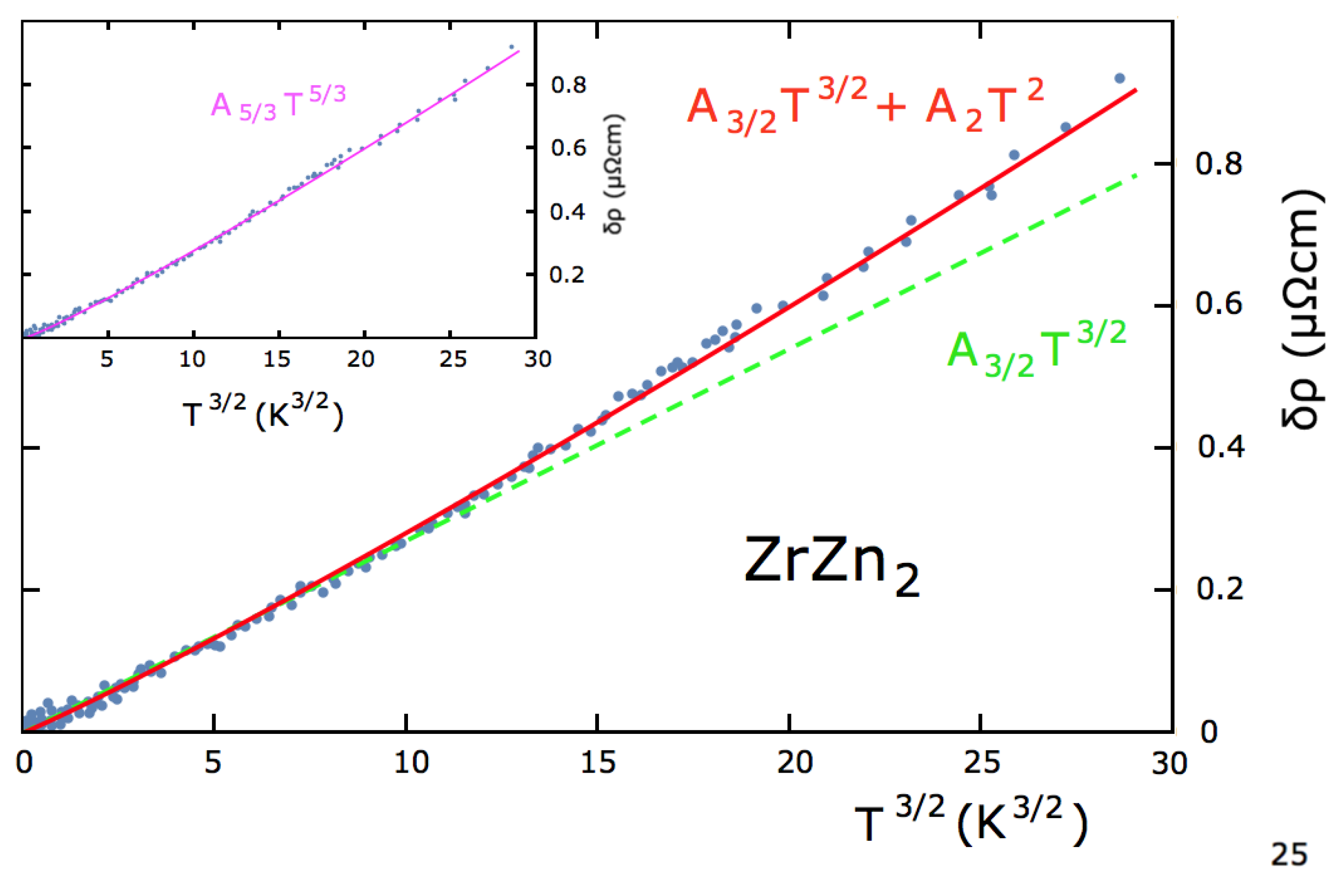
References [7,22] used s and $A_s$, as given above, and $A_2=0$ and obtained a good fit. In Figure 5, we reproduce this fit (in the inset) and compare it with a fit that uses Equation (33) with $s=3/2$, $A_{3/2}=0.021\mathsf{\mu }\Omega$cm/K${}^{3/2}$, and $A_2=0.0033\mathsf{\mu }\Omega$cm/K${}^2$ (solid red line in the main figure). There are at least two physical motivations for this: (1) in Section 4, we identified several scattering mechanisms that lead to $s=3/2$. (2) There is no reason to believe that $A_2=0$. Indeed, Reference [22] found a $T^2$ behavior in a magnetic field of 9 T with a prefactor that is very close to the one used for the fit in Figure 5. An obvious explanation is that the magnetic field gaps out the magnons which eliminates the scattering mechanism that produces $s=3/2$ and leaves a $T^2$ mechanism of unknown origin behind. It then is natural to assume that this $T^2$ mechanism is also present in a zero field and needs to be taken into account. It is very interesting that the resulting fit, the solid red line in the main figure, is of equal quality to the pure $T^{5/3}$ fit shown in the inset. Indeed, if plotted on top of one another, the two fits are indistinguishable on the scale of the figure. We conclude that the data by themselves cannot distinguish between a pure $T^{5/3}$ behavior and a $T^{3/2}$ behavior with a $T^2$ correction. A pure $T^{3/2}$ behavior, on the other hand, gives a good fit, but in a much more limited temperature regime (see the green dashed line in the figure).

In this context of multiple scattering mechanisms, we also stress again that the presence of a resistivity exponent of $s=2$ does not necessarily imply that the transport behavior is conventional. For instance, the very large value of the prefactor $A_2$ observed in the helically-ordered phase of MnSi cannot be explained by any known scattering mechanism. A related point is that a scattering mechanism leading to a smaller value of s may not dominate over one leading to a larger value unless one goes to very low temperatures, as the crossover temperature obviously depends on the ratio of the prefactors. In the helical phase of MnSi, the helimagnons (in the form of the $TlnT$ contribution mentioned at the end of Section 4.3.2) must manifest themselves at sufficiently low temperatures, but an estimate in Reference [9] suggests that they will dominate over the unknown scattering mechanism leading to $s=2$ only for temperatures below about 30 mK. The use of transport measurements in the ordered phase of MnSi to check this prediction would be very interesting.

5.4. Quenched Disorder

An important component of the discussion of systems with weak quenched disorder in Section 4.1.2 is that the disorder suppresses the backscattering factor in the expression of the transport relaxation rate. This is a qualitative argument, and a more detailed theoretical analysis of the disorder dependence of the backscattering factor and the related crossover in the T-dependence of the electrical resistivity is desirable. The same is true for the crossover from the ballistic or weak-disorder regime to the strong-disorder regime that is characterized by diffusive electron dynamics. From an experimental point of view, a more detailed characterization of disorder and how to quantify its presence is desirable. The residual resistivity may be a rather crude measure of disorder. For instance, there is experimental evidence for inhomogeneities in pressure-tuned systems that are not necessarily reflected in transport experiments and thus, can be present even in systems with a rather small residual resistivity [63].

References

- Wilson, A.H. The Theory of Metals; Cambridge University Press: Cambridge, UK, 1954. [Google Scholar]
- Kittel, C. Introduction to Solid State Physics; Wiley: New York, NY, USA, 2005. [Google Scholar]
- Gurvitch, M.; Fiory, A.T. Resistivity of La1.825Sr0.175CuO4 and YBa2Cu3O7 to 1100K: Absence of Saturation and Its Implications. Phys. Rev. Lett. 1989, 59, 1337. [Google Scholar] [CrossRef] [PubMed]
- Takagi, H.; Batlogg, B.; Kao, H.L.; Kwo, J.; Cava, R.J.; Krajewski, J.J.; Peck, W.F. Systematic Evolution of Temperature-Dependent Resistivity in La2−xSrxCuO4. Phys. Rev. Lett. 1992, 69, 2975. [Google Scholar] [CrossRef] [PubMed]
- Sato, M. Magnetic Properties and Electrical Resistivity of (Ni1−xPdx)3Al. J. Phys. Soc. Jpn. 1975, 39, 98. [Google Scholar] [CrossRef]
- Niklowitz, P.G.; Beckers, F.; Lonzarich, G.G.; Knebel, G.; Salce, B.; Thomasson, J.; Bernhoeft, N.; Braithwaite, D.; Flouquet, J. Spin-fluctuation-dominated electrical transport of Ni3Al at high pressure. Phys. Rev. B 2005, 72, 024424. [Google Scholar] [CrossRef]
- Takashima, S.; Nohara, M.; Ueda, H.; Takeshita, N.; Terakura, C.; Sakai, F.; Takagi, H. Robustness of the Non-Fermi-Liquid Behavior near the Ferromagnetic Critical Point in Clean ZrZn2. J. Phys. Soc. Jpn. 2007, 76, 043704. [Google Scholar] [CrossRef]
- Pfleiderer, C.; Julian, S.R.; Lonzarich, G.G. Non-Fermi-liquid nature of the normal state of itinerant-electron ferromagnets. Nature 2001, 414, 427. [Google Scholar] [CrossRef] [PubMed]
- Kirkpatrick, T.R.; Belitz, D. Generic non-Fermi-liquid behavior of the resistivity in weakly disordered ferromagnets and clean helimagnets. Phys. Rev. B 2018, 97, 064411. [Google Scholar] [CrossRef]
- Forster, D. Hydrodynamic Fluctuations, Broken Symmetry, and Correlation Functions; Benjamin: Reading, MA, USA, 1975. [Google Scholar]
- Ziman, J.M. Electrons and Phonons; Clarendon: Oxford, UK, 1960. [Google Scholar]
- Georgi, H. Unparticle physics. Phys. Rev. Lett. 2007, 98, 221601. [Google Scholar] [CrossRef] [PubMed]
- Pines, D.; Nozières, P. The Theory of Quantum Liquids; Addison-Wesley: Redwood City, CA, USA, 1989. [Google Scholar]
- Anderson, P.W. Basic Notions of Condensed Matter Physics; Benjamin: Menlo Park, CA, USA, 1984. [Google Scholar]
- Bharadwaj, S.; Belitz, D.; Kirkpatrick, T.R. Electronic relaxation rates in metallic ferromagnets. Phys. Rev. B 2014, 84, 134401. [Google Scholar] [CrossRef]
- Brando, M.; Duncan, W.J.; Moroni-Klementowicz, D.; Albrecht, C.; Grüner, D.; Ballou, R.; Grosche, F.M. Logarithmic Fermi-Liquid Breakdown in NbFe2. Phys. Rev. Lett. 2008, 101, 126401. [Google Scholar] [CrossRef] [PubMed]
- Lee, P.A.; Ramakrishnan, T.V. Disordered electronic systems. Rev. Mod. Phys. 1985, 57, 287. [Google Scholar] [CrossRef]
- Belitz, D.; Kirkpatrick, T.R. The Anderson-Mott transition. Rev. Mod. Phys. 1994, 66, 261. [Google Scholar] [CrossRef]
- Uhlarz, M.; Pfleiderer, C.; Hayden, S.M. Quantum Phase Transition in the Itinerant Ferromagnet ZrZn2. Phys. Rev. Lett. 2004, 93, 256404. [Google Scholar] [CrossRef] [PubMed]
- Pfleiderer, C.; McMullan, G.J.; Julian, S.R.; Lonzarich, G.G. Magnetic quantum phase transition in MnSi under hydrostatic pressure. Phys. Rev. B 1997, 55, 8330. [Google Scholar] [CrossRef]
- Brando, M.; Belitz, D.; Grosche, F.M.; Kirkpatrick, T.R. Metallic quantum ferromagnets. Rev. Mod. Phys. 2016, 88, 025006. [Google Scholar] [CrossRef]
- Sutherland, M.; Smith, R.P.; Marcano, N.; Zou, Y.; Rowley, S.E.; Grosche, F.M.; Kimura, N.; Hayden, S.M.; Takashima, S.; Nohara, M.; et al. Transport and thermodynamic evidence for a marginal Fermi-liquid state in ZrZn2. Phys. Rev. B 2012, 85, 035118. [Google Scholar] [CrossRef]
- Ishikawa, Y.; Tajima, K.; Bloch, D.; Roth, M. Helical spin structure in manganese silicide MnSi. Solid State Commun. 1976, 19, 525. [Google Scholar] [CrossRef]
- Pfleiderer, C.; Reznik, D.; Pintschovius, L.; van Löhneysen, H.; Garst, M.; Rosch, A. Partial order in the non-Fermi-liquid phase of MnSi. Nature 2004, 427, 227. [Google Scholar] [CrossRef] [PubMed]
- Pfleiderer, C. On the Identification of Fermi-Liquid Behavior in Simple Transition Metal Compounds. J. Low Temp. Phys. 2007, 147, 231. [Google Scholar] [CrossRef]
- Tewari, S.; Belitz, D.; Kirkpatrick, T.R. Blue Quantum Fog: Chiral Condensation in Quantum Helimagnets. Phys. Rev. Lett. 2006, 96, 047207. [Google Scholar] [CrossRef] [PubMed]
- Mühlbauer, S.; Binz, B.; Jonietz, F.; Pfleiderer, C.; Rosch, A.; Neubauer, A.; Georgii, R.; Böni, P. Skyrmion Lattice in a Chiral Magnet. Science 2009, 323, 915. [Google Scholar] [CrossRef] [PubMed]
- Technical University Munich Press Release. Discovery of a New Magnetic Order: Skyrmion Lattice in a Chiral Magnet. Available online: https://www.frm2.tum.de/en/news-media/press/news/news/article/discovery-of-a-new-magnetic-order-skyrmion-lattice-in-a-chiral-magnet/ (accessed on 10 October 2018).
- Fluitman, J.H.J.; Boom, R.; De Chatel, P.F.; Schinkel, C.J.; Tilanus, J.L.L.; De Vries, B.R. Possible explanations fo the low temperature resisitivities of Ni3Al and Ni3Ga alloys in terms of spin density fluctuation theories. J. Phys. F 1973, 3, 109. [Google Scholar] [CrossRef]
- Kirkpatrick, T.R.; Belitz, D. Columnar Fluctuations as a Source of Non-Fermi-Liquid Behavior in Weak Metallic Magnets. Phys. Rev. Lett. 2010, 104, 256404. [Google Scholar] [CrossRef] [PubMed]
- Kirkpatrick, T.R.; Belitz, D. Stable phase separation and heterogeneity away from the coexistence curve. Phys. Rev. B 2016, 93, 144203. [Google Scholar] [CrossRef] [Green Version]
- Kasuya, T. Electrical Resistance of Ferromagnetic Metals. Progr. Theor. Phys. 1956, 16, 58. [Google Scholar] [CrossRef]
- Goodings, D.A. Electrical Resistivity of Ferromagnetic Metals at Low Temyeratures. Phys. Rev. 1963, 132, 542. [Google Scholar] [CrossRef]
- Campbell, I.A.; Fert, A. Transport Properties of Ferromagnets. In Ferromagnetic Materials; Wohlfarth, E.P., Ed.; North Holland: Amsterdam, The Netherlands, 1982; Volume 3. [Google Scholar]
- Ueda, K.; Moriya, T. Contribution of Spin Fluctuations to the Electrical and Thermal Resistivities of Weakly and Nearly Ferromagnetic Metals. J. Phys. Soc. Jpn. 1975, 39, 605. [Google Scholar] [CrossRef]
- Moriya, T. Spin Fluctuations in Itinerant Electron Magnetism; Springer: Berlin, Germany, 1985. [Google Scholar]
- Goedsche, F.; Möbius, A.; Richter, A. On the Low-Temperature Resistivity of Ferromagnetic Transition Metal Alloys. Phys. Stat. Sol. 1979, 96, 279. [Google Scholar] [CrossRef]
- Belitz, D.; Kirkpatrick, T.R.; Rosch, A. Theory of helimagnons in itinerant quantum systems. Phys. Rev. B 2006, 73, 054431. [Google Scholar] [CrossRef]
- Belitz, D.; Kirkpatrick, T.R.; Rosch, A. Theory of helimagnons in itinerant quantum systems. II. Nonanalytic corrections to Fermi-liquid behavior. Phys. Rev. B 2006, 74, 094408. [Google Scholar] [CrossRef]
- Belitz, D.; Kirkptrick, T.R.; Saha, R. Theory of helimagnons in itinerant quantum systems. III. Quasiparticle description. Phys. Rev. B 2008, 78, 094407. [Google Scholar]
- Belitz, D.; Kirkptrick, T.R.; Saha, R. Theory of helimagnons in itinerant quantum systems. IV. Transport in the weak-disorder regime. Phys. Rev. B 2008, 78, 094408. [Google Scholar]
- Zala, G.; Narozhny, B.N.; Aleiner, I.L. Interaction corrections at intermediate temperatures: Longitudinal conductivity and kinetic equation. Phys. Rev. B 2001, 64, 214204. [Google Scholar] [CrossRef]
- DeGennes, P.G.; Prost, J. The Physics of Liquid Crystals; Clarendon: Oxford, UK, 1993. [Google Scholar]
- Ho, K.; Kirkpatrick, T.R.; Sang, Y.; Belitz, D. Ordered Phases of Itinerant Dzyaloshinsky-Moriya Magnets and Their Electronic Properties. Phys. Rev. B 2010, 82, 134427. [Google Scholar] [CrossRef]
- Petrova, O.; Tchernyshyov, O. Spin waves in a skyrmion crystal. Phys. Rev. B 2011, 84, 214433. [Google Scholar] [CrossRef]
- Hertz, J. Quantum Phase Transitions. Phys. Rev. B 1975, 14, 1165. [Google Scholar] [CrossRef]
- Mathon, J. Magnetic and Electrical Properties of Ferromagnetic Alloys Near the Critical Concentration. Proc. Roy. Soc. Lond. Ser. A 1968, 306, 355. [Google Scholar] [CrossRef]
- Millis, A.J. Effect of a nonzero temperature on quantum critical points in itinerant fermion systems. Phys. Rev. B 1993, 48, 7183. [Google Scholar] [CrossRef]
- Kirkpatrick, T.R.; Belitz, D. Exponent relations at quantum phase transitions, with applications to metallic quantum ferromagnets. Phys. Rev. B 2015, 91, 214407. [Google Scholar] [CrossRef]
- Kirkpatrick, T.R.; Belitz, D. Quantum critical behavior of disordered itinerant ferromagnets. Phys. Rev. B 1996, 53, 14364. [Google Scholar] [CrossRef]
- Belitz, D.; Kirkpatrick, T.R.; Mercaldo, M.T.; Sessions, S. Quantum critical behavior in disordered itinerant ferromagnets: Logarithmic corrections to scaling. Phys. Rev. B 2001, 63, 174428. [Google Scholar] [CrossRef]
- Kirkpatrick, T.R.; Belitz, D. Pre-asymptotic critical behavior and effective exponents in disordered metallic quantum ferromagnets. Phys. Rev. Lett. 2014, 113, 127203. [Google Scholar] [CrossRef] [PubMed]
- Goko, T.; Arguello, C.J.; Hamann, A.; Wolf, T.; Lee, M.; Reznik, D.; Maisuradze, A.; Khasanov, R.; Morenzoni, E.; Uemura, Y.T. Restoration of quantum critical behavior by disorder in pressure-tuned (Mn,Fe)Si. NPJ Quantum Mater. 2017, 2, 44. [Google Scholar] [CrossRef]
- Landau, L.D. The theory of a Fermi liquid. Zh. Eksp. Teor. Fiz. 1956, 30, 1058. [Google Scholar]
- Landau, L.D. Oscillations in a Fermi liquid. Zh. Eksp. Teor. Fiz. 1957, 32, 59. [Google Scholar]
- Landau, L.D. On the theory of the Fermi liquid. Zh. Eksp. Teor. Fiz. 1958, 35, 97. [Google Scholar]
- Silin, V.P. Theory of a degenerate electron liquid. Zh. Eksp. Teor. Fiz. 1957, 33, 459. [Google Scholar]
- Schulz, H. Fermi liquids and non-Fermi liquids. In Proceedings of the Les Houches Summer School LXI; Akkermans, E., Montambqux, G., Pichard, J., Zinn-Justin, J., Eds.; Elsevier: Amsterdam, The Netherlands, 1995. [Google Scholar]
- Varma, C.M.; Littlewood, P.B.; Schmitt-Rink, S.; Abrahams, E.; Ruckenstein, A.E. Phenomenology of the Normal State of Cu-O High-Temperature Superconductors. Phys. Rev. Lett. 1989, 63, 1996. [Google Scholar] [CrossRef] [PubMed]
- Pal, H.K.; Yudson, V.I.; Maslov, D.L. Resistivity of Non-Galilean-Invariant Fermi- and Non-Fermi Liquids. Lith. J. Phys., 2012, 52, 142. [Google Scholar] [CrossRef]
- Belitz, D.; Kirkpatrick, T.R.; Vojta, T. How generic scale invariance influences quantum and classical phase transitions. Rev. Mod. Phys. 2005, 77, 579. [Google Scholar] [CrossRef]
- Sachdev, S. Where is the quantum critical point in the cuprate superconductors? Phys. Status Solidi B 2010, 247, 537. [Google Scholar] [CrossRef] [Green Version]
- Yu, W.; Zamborsky, F.; Thompson, J.D.; Sarrao, J.L.; Torelli, M.E.; Fisk, Z.; Brown, S.E. Phase inhomogeneity of the itinerant ferromagnet MnSi at high pressures. Phys. Rev. Lett. 2004, 92, 086403. [Google Scholar] [CrossRef] [PubMed]
Figure 1.
(Left) panel: Observed temperature–pressure phase diagram of ZrZn, with the false colors indicating the value of the resistivity exponents. The white lines represent lines of second-order (solid) and first-order (dashed) transitions between the ferromagnetic (FM) and paramagnetic (PM) phases, and TCP denotes the tricritical point where the order of the transition changes. Based on Figure 2 in Reference [7]; this version was taken from Reference [9]. (Right) panel: Measured resistivity of MnSi in the nonmagnetic phase (based on Reference [8]).
Figure 2.
(Left) panel: Temperature–pressure phase diagram of MnSi based on experimental data from References [20,24,25] and theoretical interpretations from Reference [26]. HM and PM denote the helimagnetic and paramagnetic phases, respectively, and NFL denotes the region where . The upper limit of the NFL region is not sharp. TCP is the observed tricritical point that separates second-order HM–PM transitions (solid line) from first-order ones (dashed line), and CP is a critical point that was proposed in Reference [26]. The inset shows the abrupt change in the resistivity exponent at the critical pressure (from Reference [9]). (Right) panel: Magnetic field–temperature phase diagram of MnSi, showing various phases. The A-phase hosts a columnar skyrmionic spin texture. The inset shows an artist’s rendition of the skyrmions in a plane that is perpendicular to the columns. Based on Figure 1 in Reference [27] (main figure); inset taken from Reference [28].
Figure 3.
(Left) panel: Electrical resistivity of NiAl plotted vs. for pressure values below, close to, and above the critical pressure (). Based on Figure 4 in Reference [6]. (Right) panel: The resistivity exponents for NiAl with a range of Ni concentrations. Data taken from Reference [29] as replotted in Reference [25]. Based on Figure 3 in Reference [25].
Figure 4.
Hexagonal lattice of columns and fluctuations about this state. a is the lattice constant, and is the displacement vector (based on Figure 5 in Reference [44]).
Figure 5.
Resistivity data (blue dots) of ZrZn vs. at ambient pressure. Data (blue dots) are taken from Figure 4 of Reference [7]. The solid red line is a fit using Equation (33) with , cm/K, and cm/K. The dashed green line is a pure fit with cm/K. The inset shows a pure fit with cm/K. On the scale of the figure, this fit is indistinguishable from the red line in the main figure.
© 2018 by the authors. Licensee MDPI, Basel, Switzerland. This article is an open access article distributed under the terms and conditions of the Creative Commons Attribution (CC BY) license (http://creativecommons.org/licenses/by/4.0/).
Share and Cite
MDPI and ACS Style
Belitz, D.; Kirkpatrick, T.R. Anomalous Transport Behavior in Quantum Magnets. Condens. Matter 2018, 3, 30. https://doi.org/10.3390/condmat3040030
AMA Style
Belitz D, Kirkpatrick TR. Anomalous Transport Behavior in Quantum Magnets. Condensed Matter. 2018; 3(4):30. https://doi.org/10.3390/condmat3040030
Chicago/Turabian StyleBelitz, Dietrich, and Theodore R. Kirkpatrick. 2018. "Anomalous Transport Behavior in Quantum Magnets" Condensed Matter 3, no. 4: 30. https://doi.org/10.3390/condmat3040030