
Statistical Inference for Visualization of Large Utility Power Distribution Systems
†


1
Department of Electrical and Electronic Engineering, Universidad de los Andes, Bogotá DC 111711, Colombia
2
Department of Electrical and Computer Engineering Science, The University of Texas at Austin, Austin, TX 78712, USA
*
Author to whom correspondence should be addressed.
†
This paper is an extended version of our paper published in Visualization of Time-Sequential Simulation for Large Power Distribution Systems. In Proceedings of the IEEE Power and Energy Society PowerTech Conference, Manchester, UK, 18–22 June 2017.
Inventions 2017, 2(2), 11; https://doi.org/10.3390/inventions2020011
Submission received: 1 March 2017
/
Revised: 28 May 2017
/
Accepted: 30 May 2017
/
Published: 8 June 2017
(This article belongs to the Special Issue Inventions and Innovation in Integration of Renewable Energy Systems)
Abstract
:Electrical variable visualization has been widely applied to report the performance and effectiveness of novel devices and strategies in utility power distribution systems. Many graphical alternatives are useful to demonstrate critical characteristics of distribution systems such as voltage regulation or power flow. This visualization of electrical variables can also be an effective approach to analyze, compare and evaluate large-scale systems. However, there is a lack of generalized visualization strategies oriented to perform electrical validations of smart grid strategies in large distribution systems. In this paper, we show that the proposed probabilistic density evolution is a powerful resource for long-term time-sequential simulations. Examinations with an IEEE 8500 node test feeder shows that the proposed approach increases the circuit situational awareness and reduces the validation time. To illustrate this methodology, the dynamic voltage condition was simulated and analyzed to recognize the global effect of voltage regulating equipment. The results show an accurate and convenient support that can be interpreted at first glance. The proper use of long-term field measurements and short time-step simulations is a robust method for future grid research, such as designing an optimum operation of intelligent devices or diagnosing electrical interoperability issues in complex grids.
1. Introduction
The inclusion of renewable energies, renewed goals for efficiency and reliability, and the technological change in the grid lead to a significant complexity in utility power distribution systems. This evolution has been reflected as a challenge for traditional approaches of simulation, validation, and design, where a plethora of scenarios and technologies demand highly efficient tools of analysis and research [1,2]. This phenomenon has increased the interest in flexible validation of strategies and equipment, but, at the same time, has led to an increment in the time and skills required to achieve an accurate interpretation of results in scenarios of interest.
For future distribution systems, it is expected that many control dynamics will be coexisting with the traditional electrical dynamic of the grid. Since most of the aggregated complexity is related to the dynamics of automatic devices [3], the analysis has been widely approached with simulations on the frequency and temporal reference frames. In particular, the time-sequential simulation is highlighted as a resource that mimics the real performance of multiple control dynamics in the system, while the results provide powerful evidence to obtain an optimum application of intelligent devices.
However, analyzing results of large-scale power distribution systems is a complex exercise, and many visualization techniques have been designed for demonstration purposes rather than a systematic analysis of data results. There are two traditional kinds of graphical visualization for distribution automation systems [4]. One category consists of one-line diagrams, while another includes geographical plots of electrical variables. Both cases display the grid status with success, but it is rarely possible to properly support the analysis of time-sequential validations.
Numerous validation strategies for large utility power distribution systems have been analyzed, where the main applications and research challenges have been identified to address the most significant visualization needs. This enlightening overview shows that the new generation of validation requirements can be substantively improved by graphical techniques. The power system operation has been historically aware of this fact, with many developments to provide visualizations that increase the data interpretation at the control center. As most of the control center visualizations focus on the instantaneous status of the system, they are not capable of representing the technical differences unleashed by a long-term consideration over a set of alternatives. However, visualization techniques for validation based on time-sequential simulations can be inspired by long-term requirements in other knowledge fields, such as meteorology, medicine, and finances. The literature review shows that there is a lack of visual techniques to analyze the temporal evolution of abundant electrical variables in large distribution systems, thus there is a fascinating research opportunity that can be focused on the finding of methodological tools to deal with the particular physical conditions of this problem.
In this paper, a detailed review of validation strategies is presented to identify current challenges for validation of future distribution systems. Focusing on graphical resources, this paper proposes a meaningful visualization technique for validation based on time-sequential simulation and statistical inference. The approach has been developed based on the nonparametric modeling of electrical results obtained by simulation. In this way, millions of simulation results are statistically processed to obtain a quantitative and succinct representation in an innovative figure, and the global perspective of long-term simulations is successfully represented.
The proposed method is intended to significantly improve the validation approach of technological development on the grid. This method allows researchers and designers to analyze the general impact on the distribution system considering an amount of information that is not feasible to depict by traditional methods. In this perspective, research on the integration of renewable energy systems and other new generation challenges can be approached with a comprehensive consideration of abundant dynamic electrical variables instead of constrained analysis over a data subset. Since the proposed method is conceived to use the temporal reference frame, offline and real-time simulations can provide detailed evidence for validation of large distribution systems. In offline simulation, this visualization technique enhances the statistical interpretation by means of the proposed formulation of non-parametric density functions. In this context, challenging conditions as the effects of high impedance faults or minor adjustments on regulating equipment can be perceived and analyzed even in long-term simulations [5,6]. On the other hand, the real-time scenario is significantly improved with the provision of specific temporal frames in which the electrical phenomena are relevant to perform electrical studies with timeliness and accuracy.
The paper is organized as follows. Section 2 presents a review as background on validation and visualization strategies for large distribution systems. Section 3 includes an original approach to visualize and support large-scale validations based on probabilistic estimation. Section 4 provides an exemplification and discussion of the density evolution applied to a few operational conditions on a large test feeder. Finally, Section 5 presents conclusions of this approach.
2. Analysis and Validation in Multi-Agent Smart Grids
The smart grid concept has been rapidly evolving to support a wide variety of goals. Interestingly, there are at least two constant components visualized by most roadmaps and current researchers. First, multiple controlled agents will be included in the traditional infrastructure; and, second, the interoperability of those devices is a significant source of risk that should be tackled. Although this is a common interest in many standardization efforts, there exists no unique methodology to validate and detect possible interoperability flaws in large-scale smart grids.
Table 1 summarizes a review of common simulation strategies applied to validate large-scale distribution systems. This compendium illustrates some successful uses of computer-aided simulations and the emergent trend to examine graphical results on large system studies. In the table, the second column refers to the maximum number of voltage nodes calculated in each study. The review shows that the complexity of models with more than 5000 is usually representative to draw conclusions about the effectiveness of larger systems. For simulations with electrical interfaces (i.e., real-time), this number is usually restricted by the computational power required by large models; however, a simplified model with a low number of electrical nodes can be useful to explore the main phenomena in certain studies.
The classification of electrical simulation strategies is contained in columns three to five. Most simulations can be classified in terms of temporal characteristics as snapshot or time-sequential. Nevertheless, the real-time simulation is gaining relevance in this topic and the list has an independent column to differentiate this particular case of time-sequential simulations.
Determining the right validation variable can only be decided in the context of each particular study, as can be seen from columns six to nine, which contain independent classifications for voltage, current, power and other variables. The latest combines complementary variables such as temperature, computational time, control device’s settings, and iterations. In this perspective, the analysis of voltage conditions remains the most frequent strategy of validation, since it is a valuable quality of service indicator. Current and power variables tend to be applied for specific studies, but the analysis and visualization of voltages are the most common components of validation.
In general, the visualization of electrical variables is simultaneously evolving with the number of agents in the grid. As can be observed in the latest two columns, figures and tables have a balanced presence in validation studies. Traditionally, the employment of figures for electrical variables is a powerful tool to exemplify important phenomena, while tables are applied to synthesize abundant data. Nonetheless, multi-agent validations usually include analysis of graphical results to create awareness of effectiveness or detect flawed operations. References included in this review show that the visualization of numerous agents in large systems is a common issue. As can be observed in the following sections, solving this challenge offers big benefits in a wide range of applications.
2.1. Time-Sequential Simulation
There are many studies that employ simulation platforms to obtain a snapshot of electrical variables at a certain system’s condition. Studies [7,8,10,11,12,13,14,15,17,18,24,25,27,29] show the application of this approach to validate proposed strategies or devices. In summary, the following are examples of typical applications for snapshot analysis and validation:
- Alternative solution methods;
- Fault location;
- Network reconfiguration;
- Power quality;
- Short-circuit analysis;
- State estimation;
- Steady state power flow;
- System’s planning;
- System’s reliability;
- Voltage regulation.
However, time-sequential simulations are essential for interoperability validation and other time dynamic phenomena. For instance, studies [7,9,14,15,16,19,20,21,22,23,24,26,27,28,30] show that the information obtained from this approach is compelling evidence for design and corroboration in many applications. In summary, the following are growing uses of time-sequential simulations in smart grid studies:
- Advanced voltage control technologies;
- Controller’s interoperability;
- Custom power devices;
- Cyber-physical analysis;
- Distributed control schemes;
- Distributed generation;
- Distribution management strategies;
- Electric transportation analysis;
- Energy efficiency improvements;
- Energy storage;
- Maintenance scheduling;
- Microgrid operation;
- Power systems communications;
- Resiliency and protection;
- Smart metering applications.
It is possible to classify several time-sequential simulation approaches in terms of the ratio of computation time over simulated time. Coefficients greater than one imply that the computational platform requires more time to solve the model than the simulated time for the power system (e.g., traditional transitory simulations). Other approaches have coefficients lower than one, and provide results of months or years of analysis in short computational times (e.g., steady state or continuous power flow); and finally, the real-time (RT) alternatives are synchronized in terms of time frames, providing a different perspective of results that could even include real equipment or users’ responses (hardware in the loop—HIL, and human in the loop—HITL). Inevitably, each category implies diverse theoretical methods that lead to interesting computational challenges.
Some studies require a high resolution in simulation’s time-step. In this case, a small time-step represents not only a computational challenge at solving models but also a big amount of data to analyze. The resulting amount of data from time-sequential simulations of large distribution systems challenges the efficiency of most analysis and simulation techniques [1]. The scale of this problem can be easily exemplified by the continuous power flow solution of the IEEE 8500 node test system. If this 2354-loads test case is simulated with one-second resolution, the power flow provides 17.6 × 10⁶ voltage computation results in one hour of operation, 421.3 × 10⁶ for one day, and 153.8 × 10⁹ for one year. The comparative analysis of multiple operative conditions usually requires independent simulations; therefore, the validation based on long-term simulation is restricted by the capability to generate, process and analyze big amounts of data. This characteristic of time-sequential simulations constitutes a major challenge for validations on future distribution systems.
2.2. Real-Time Simulation
The time-sequential simulation has been successfully employed by real-time simulators as a tool to support the design, analysis, and validation processes in power systems [31]. In this approach, powerful computational platforms can be employed as dedicated simulation devices to enhance the simulator’s flexibility. Therefore, the validation core relies on a computational platform with advanced signal processing capabilities to reproduce the electrical signals provided by continuous computational simulations. The number of validation developments based on real-time simulation has been increasing as a result of the potential capability in many research topics of power systems. Some research centers have successfully deployed this method [9,19,21,22,23,26,28,30], and powerful power systems laboratories are obtaining a growing role as the next generation of validation for smart grids. The increasing development of powerful computational platforms increases the potential application of studies with large distribution systems, where the solving process has challenging scales.
2.3. Visualization of Large Utility Power Distribution Systems
The visual analysis of electrical variables is one powerful approach usually applied to recognize patterns, to validate assumptions, and to perceive the evolutive effects of a system’s dynamics that could be difficult to abstract from mathematical representations. However, the visualization of electrical variables in large distribution systems is characterized by the physical restriction of a figure’s space, leading to summarization of data in tables or selecting only the most significant data to visualize. Since most of the validation process in future strategies for smart grids is focused on innovative schemes, it is convenient to use the basic principle of visualization to explore unexpected events in large systems.
This section shows some traditional alternatives of visualization based on the IEEE 8500 nodes distribution system. This test feeder was simulated to obtain the voltage magnitude of the 2354 loads with the purpose of recognizing the voltage condition with traditional volt/var regulating equipment. Other details of the simulation are omitted for the purpose of this exemplification.
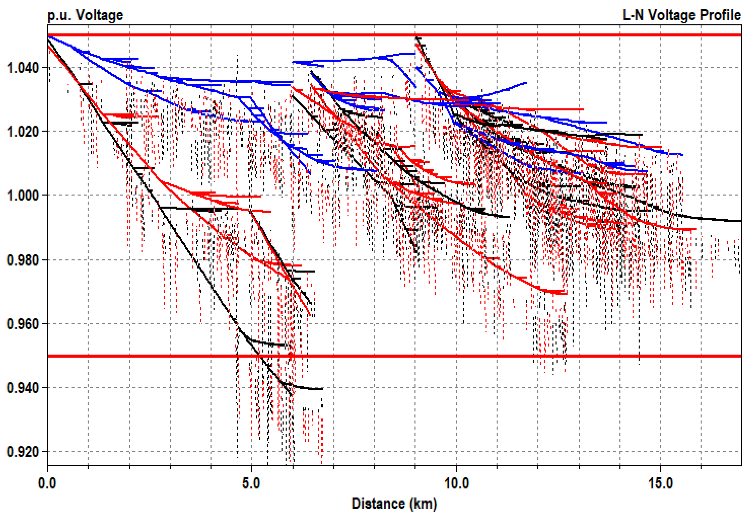
Figure 1 and Figure 2 show two geographical representations of voltage magnitude in the test system. Both visualizations are based on the same snapshot condition in the system. In Figure 1, the voltage magnitude range is associated with a color scale, and the geographical topology is used to show a colorful interpolation of the simulated data. An alternative visualization (Figure 2) uses the Cartesian reference to show the voltage magnitude in the vertical axes and the distance from the substation to each location in the horizontal axes (commonly known as voltage profile). The geographical component of these figures is useful to associate the events with equipment allocation and diverse conditions. Nevertheless, Figure 1 and Figure 2 include data of one circuit condition, and representation of the temporal performance is highly restricted with these approaches.
Data from time-sequential simulations can be represented with two-dimensional (2D) and three-dimensional (3D) visualizations. As can be seen in Figure 3, the three-dimensional representation of load voltages can be used to observe the temporal evolution of the system, but the amount of results in large simulations is a major restriction to analyze events, to draw conclusions, or to locate singularities. In a broader perspective, the use of 3D supplies a general overview of the system, where the color scale suggests the major trends in results. This methodology can be applied to compare and detect relatively significant changes in large simulations, or as a resource to detect the existence of results highly deviated from the main trend. In this particular example, it is possible to conclude that the system’s operation does not show any events of critical change, although some nodes are improperly subject to low voltage magnitude (i.e., less than 0.95 ) on certain time instants.
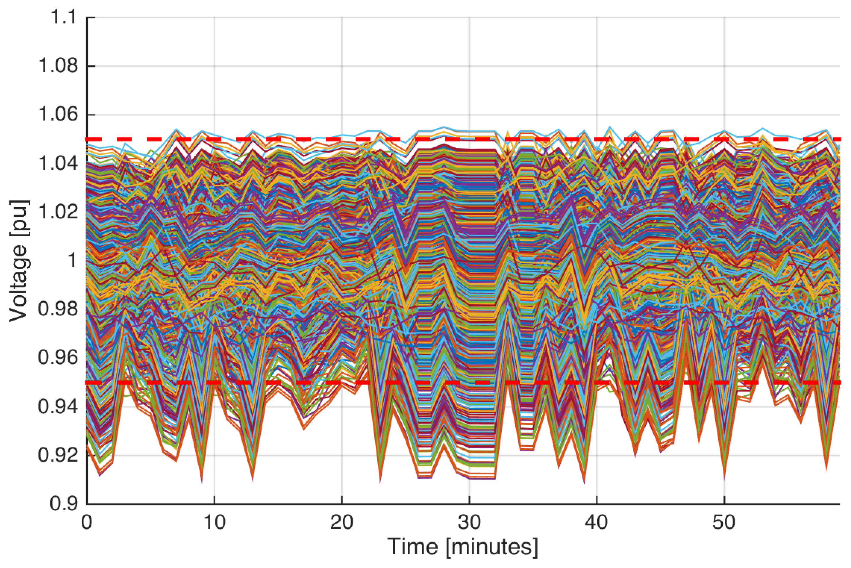
The flat or 2D visualization of the same large simulation only provides information about maximum and minimum limits in the variable of interest. Figure 4 shows an example of the 2D representation for the previously discussed simulation. In this case, the amount of lines associated with each variable harms the identification of trends inside the limits. On the other hand, the minimum and maximum boundaries are clearly depicted and main conclusions can be extracted from this information. In this example, the simulation shows that some loads were supplied with high voltage magnitudes, exceeding the regulatory limit of 1.05 Vpu. Similarly, the lower voltage limit is certainly defined, where the improperly low magnitude is evident for most of the simulated frame. Other details about the internal tendency or amount of loads with certain magnitudes remain uncertain with this approach.
The selection of representative data is one natural alternative to this methodology, although the detection of significant data in large distribution systems is one of the initial motivations to use data visualization. One possible approach consists of a previous processing of simulation results, with the purpose of identifying a subset of variables that meets certain conditions of interest. In the example of voltage visualization, it is possible to select and plot only the loads with minimum and maximum voltage; however, the extreme voltage conditions are not always associated with the same loads in a time-sequential simulation. The following section describes this particular phenomenon to highlight the influence of circuit’s variability in the visualization of large distribution systems.
2.4. The Problem of Worst Voltage Condition Allocation
The variability of voltage conditions in secondary circuits (i.e., 120 or 240 ) is an illustrative example of the complexity of voltage analysis for time-sequential simulations.
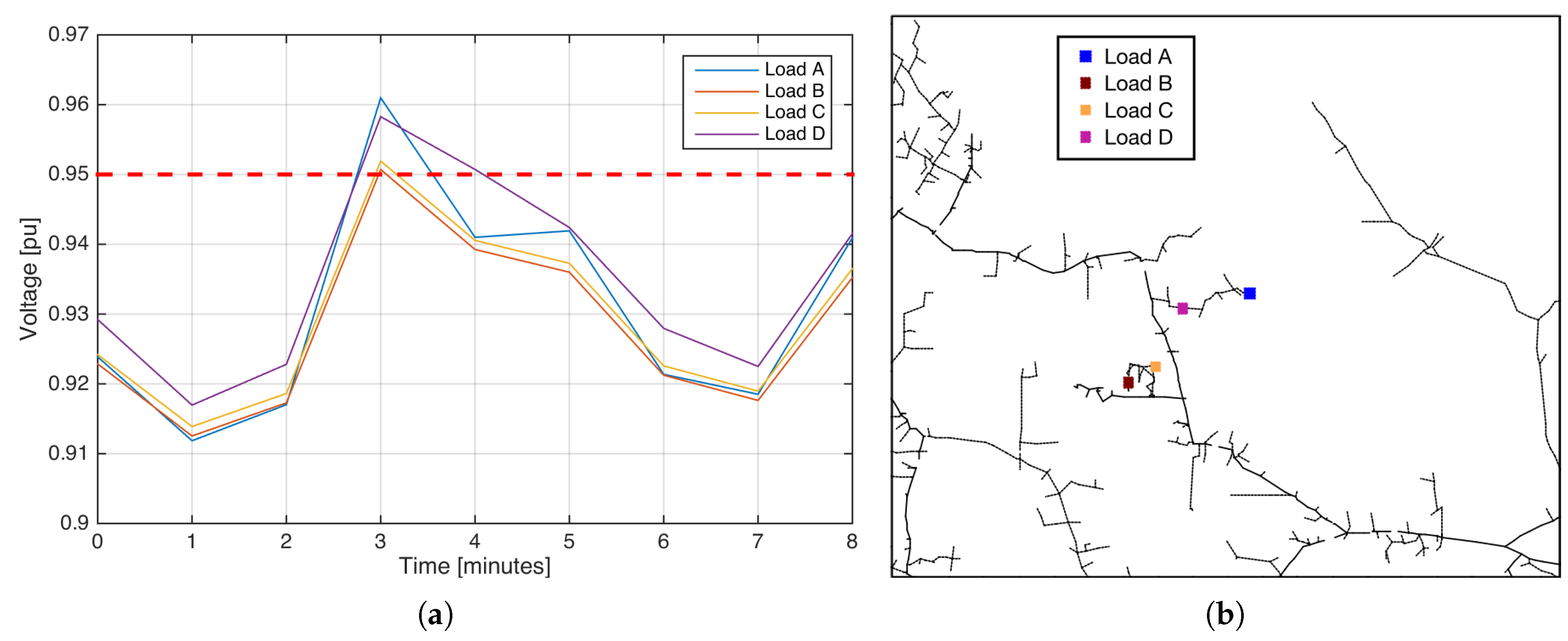
The selection of locations of interest is a frequent approach to reducing the number of signals in large distribution systems; however, the consumption variability induces an important effect in the secondary circuit, inducing a misleading identification of singular locations. As can be seen in Figure 5a, the lower voltage in the simulated distribution system is not statically associated with one particular location. In this scenario, four loads with low voltage magnitude were selected to perform eight minutes of simulation and to illustrate the effect of voltage variability in secondary circuits. The minimum voltage occurs at minute one, when Load A is supplied with Vpu. At this point, it is possible to conclude that the voltage magnitude of Load A is representative, as it exhibits the minimum voltage in the simulated time frame, but the detailed examination of other voltages shows that Load B has the lower voltage in the circuit for the remaining time instants. In this example, the analysis based on one location that exhibits the minimum voltage in the simulated frame omits the fact that other locations have regulating problems when Load A is properly supplied (e.g., Load B at minute 3).
The geographical location is another option to define the load of interest. Figure 5b shows the location for the same four selected loads. Load A and Load D are located in the same primary section of the simulated circuit. For this pair, it seems reasonable to conclude that Load A will be supplied with lower voltages’ magnitudes due to the location at the end of the primary section, and the absence of other regulating equipment in this area. Surprisingly, the simulation shows that there are circumstances where Load D has lower magnitude than Load A (see minute 3). The origin of this phenomenon resides in the variability of voltage drops in secondary circuits as a result of variable consumptions and balance conditions, among others.
This electrical condition obstructs a clear validation when figures are based on visualization of selected locations of interest. Other sources of variability are frequently included in smart grid validations; for instance, controlled equipment, nonlinear loads, protection devices, distributed generation, and energy storage, among others. Therefore, it is useful to apply the basic principles of data analytics to discover useful information in a large amount of data from time-sequential simulations. The following section describes a proposed approach for visualization of significant tendencies in voltage magnitude for large distribution systems.
3. Meaningful Visualization for Voltage Analysis
Validation of distribution systems’ operation usually includes the analysis of quality of service in terms of voltage magnitude for final users. One of the most frequent references of validation consists of a direct comparison between simulated voltages and ANSI C84.1 limits for service voltages. This validation is not only relevant to detect possible harmful situations for final users (e.g., over-voltages in steady-state condition), but also to compare the perceived performance of the grid in front of base scenarios or alternatives.
In this section, the application of statistical inference and a proposed visualization of time-sequential simulations are described. Traditional sources of uncertainty in the model imply the need for a statistical interpretation of simulation results; therefore, the visualization of probabilistic density functions obtained from simulated data provides an estimation of the circuit’s performance. This estimation aims to depict the evolution of the system’s dynamic as a validation tool that could be used to locate singular conditions or analyze detailed simulations. However, the probabilistic distribution resulting from the grid’s components is not static in time, and the parameter estimation of traditional probabilistic distributions conduces to significant flaws in the validation process.
3.1. Statistical Inference
In statistical terms, simulation results for load voltages are a population or complete set of elements, where the statistical inference has no apparent purpose; however, each electrical simulation is performed with multiple uncertainty factors, and analysis of solutions aims to draw conclusions about the real electrical scenario. Sources of uncertainty are related to the availability of information to properly model conductors and other grid’s elements, but they are also related to the lack of details to reproduce the random consumption of each load in large systems. In this perspective, the complete set of results from each simulation is a statistical sample of the system, and multiple methods of statistical inference can be applied.
In this proposed approach, the estimation of the probability density function (PDF) is performed by means of the kernel density estimation (KDE). This non-parametric method is used to support the inference process in simulated data with multimodality or uncertain distributions. In this way, the estimation produces a probabilistic distribution function based on the finite sample data without the presumption that the system can be modeled with parametric distributions as Weibull, normal, exponential, etc.
The univariate kernel estimator of f is defined as (1), where are points in the finite sample, K is the kernel function, and h is the bandwidth:
It is possible to apply multiple symmetric distributions as the K function; however, this is known as a factor with low impact in the estimation. Based on tests and validations with the mean integrated squared error, it is possible to conclude that the Gaussian kernel density estimator (2) provides an adequate estimation in the application to large distribution systems:
On the other hand, the bandwidth selection has a significant influence on the asymptotic properties of the estimation. Selection of h could be driven by the minimization of the mean integrated squared error, with the popular approximation (3), where is the standard deviation of the samples. Effectiveness of the approximation is related to the outliers’ characteristics. The analysis of normalized voltage magnitudes in large distribution systems suggests that the approximation is adequate for this application. This conclusion was also validated by experimental comparisons with alternative methods for bandwidth selection [32], where the results show that the approximation is accurate for estimation of the voltage magnitude distributions:
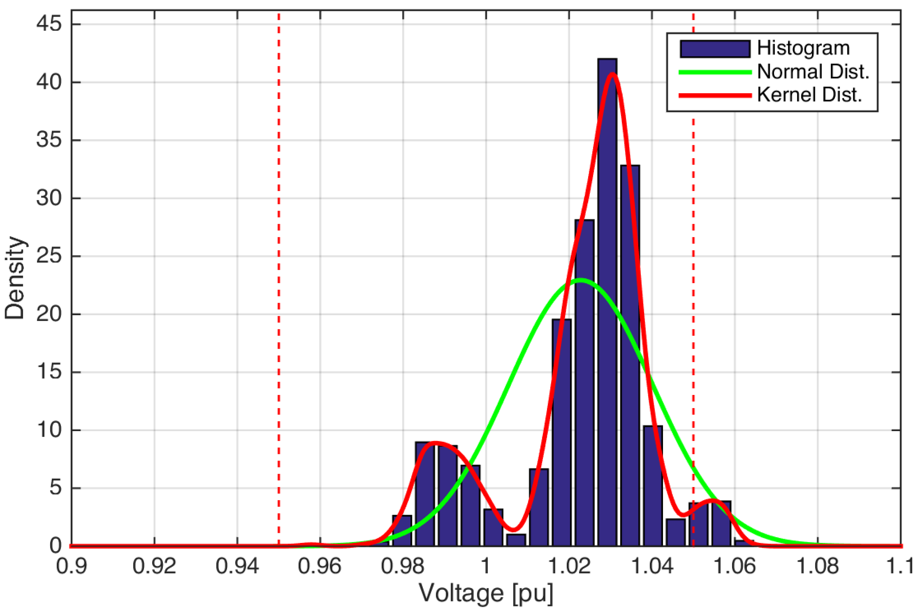
Figure 6 shows the application of this method to estimate the density function that describes load’s voltage magnitude in the IEEE 8500 test feeder for certain load conditions. The histogram of the normalized amplitudes exhibits three local groups of density, with approximate centers in 0.99 , 1.1 , and 1.055 . The green line shows the estimation of this sample with the normal probability function, and the red line shows the result of the kernel estimation. As can be seen, the kernel distribution has a proper fitting to the sampled data, and it is possible to draw appropriate conclusions of voltage conditions. In contrast, the normal approximation has a significant error and the consequent inference is not reliable.
The kernel estimation of electrical variables in large distribution systems is useful to detect conditions of interest. As a result, the information provided by the estimated density function can be used to trace possible causes of undesired conditions and validate the effect of posterior changes. In the case of voltage magnitude (e.g., Figure 6), the presence of local density peaks could be used to identify common voltage conditions in the system; next, the simulation results can be filtered to locate the loads and geographical areas with those particular conditions; then, mitigation actions can be applied for locations with undesired conditions, and finally, the simulation with mitigation alternatives provide additional samples that can be estimated with the kernel function to compare with the original density function. This comparison of density functions provides information to validate the effectiveness of each alternative in one particular system’s condition (e.g., time instant, load condition, regulator taps, among others).
3.2. Time Sequential Visualization
An efficient visualization of the system’s evolution leads to a proper drawing of conclusions in design or validation processes. The proposed approach is simple to reproduce with a variety of electrical variables, yet it is powerful as an analysis tool to synthesize the system’s evolution. Here, the approach is documented as a particular application for analysis of voltage magnitude; however, the methodology can be applied for analysis of other variables of interest in each particular validation study.
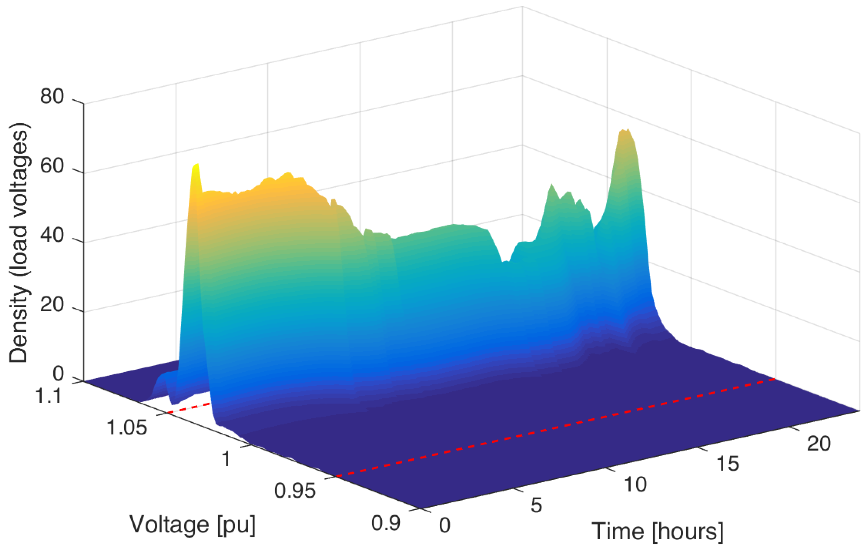
Kernel density functions show the system’s condition at a particular condition or time instant. The estimation for multiple steps shows the evolution of those conditions in the desired temporal frame. 3D representations of the density evolution use the t-axes to plot each estimation and depict the graphical pattern of changes.
The bivariate kernel distribution used in the proposed visualization is described by (4), where are results at time t, is the bandwidth for samples at time t, and is the standard deviation at the same time-step t:
This calculation is performed for each time-step in a time-sequential simulation. With the resulting set of PDFs for the desired time frame, a three-dimensional figure of probabilistic characteristics is produced (Figure 7). Different details of the process are abstracted from the generated surface by rotation of the 3D representation.
Some details are not evident in certain perspectives, as the time-sequential simulation provides data of the complex system’s dynamics. In a broader context, the two-dimensional projection of the density evolution plot reports comparable information with a convenient presentation. The contour projection is obtained from and color scales can be used to associate diverse density levels in the plot. The 2D visualization is also convenient to include additional and complementary curves. In the voltage visualization case, the ANSI C84.1 magnitude limits are overlapped to facilitate the abstraction of interesting phenomena. Unlike the 3D view, this 2D representation shows the system’s conditions for each time step at first sight. The following section shows the 2D evolution applied on the test case.
4. Test Case on Large Feeder and Discussion
The analysis is based on the IEEE 8500 node test feeder. This radial feeder considers the medium and low voltage levels in the model, with 2354 unbalanced loads, three voltage regulators, four capacitor banks and one load tap changer at the substation’s transformer. The realistic features of this moderately large system are intended to prove the ability of system analysis algorithms with large scale problems [33]. For this analysis, the 8500 node circuit was configured in accordance with the normal operation condition. Therefore, the line drop compensators (LDC) and capacitor controllers are in service with the settings provided by the Test Feeders Working Group (WG) of the Distribution System Analysis Subcommittee of the Power Systems Analysis, Computing, and Economics (PSACE) Committee.
The test system definition does not include information about the temporal behavior of the loads; therefore, external load shapes were normalized and applied to the model to obtain a realistic change of power consumption for one year of operation with one-minute resolution. The applied load shapes are independent for phases A and B, reproducing a wide range of load conditions for different seasons in one year. This set of scale factors is based on the information provided in [34].
Time-sequential simulations were performed with the OpenDSS platform (Version 7.6.5.18, Electric Power Research Institute—EPRI, Palo Alto, CA , USA) [35]. OpenDSS includes a wide gallery of device models aimed to analyze the automation operation in distribution systems. The following results were obtained from the software implementation of the proposed approach with MATLAB® (Version 8.6.0, The MathWorks, Natick, MA, USA) in co-simulation with OpenDSS.
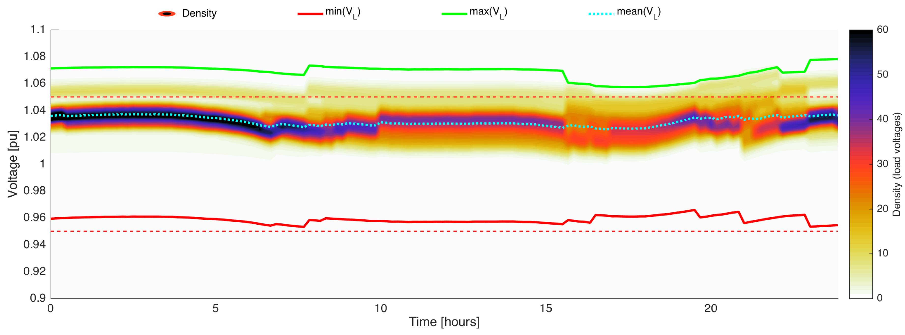
Figure 8 shows the density evolution of load’s voltage magnitudes from a 24 h simulation in the IEEE 8500 nodes test feeder. The color bar on the right side of the figure is associated with the contour visualization of , where are the load voltage results from the time-sequential simulation; additionally, the minimum and maximum voltages of each time-step (, ) are plotted in red and green lines. The blue-dashed line corresponds to the average of the sample () over time.
As can be seen in this example, the highest densities in voltage magnitude (i.e., the most frequent voltage magnitudes estimated by the PDF) are in the range from 0.97 to 1.05 , but the voltage condition is not constant through the simulated period. The visual strip delimited by the minimum and maximum voltages describes the range . It is important to notice that some internal areas near the limits are white colored to represent low probabilistic density, but there is at least one simulated voltage with a value equal to the visual boundary (red and green lines). The figure shows that the over voltage is the main voltage violation in the system, as the density strip has maximum voltages over 1.05 most of the time, and the under voltages are only evident between the 14 and 18 h. Moreover, the density evolution shows that there are concentrated voltages with an approximate magnitude of 1.03 for the first 10 , and the increased dispersion in subsequent hours is also evident. Sudden changes in density are evident in the figure leading to fast detection of conditions of interest (e.g., rise of high-density magnitude at hour 18, and high dispersion at hour 16).
The visualization of 24 of electrical results, which represents the dynamic voltage condition of 2354 loads, has been shown in Figure 8. The reader is not only aware of a set of temporal effects of the voltage regulating equipment in this large system, but also the massive amount of data can be easily compared with candidate adjustments or improvements. For instance, it is possible to observe that the regulating equipment takes corrective actions at hour 16. In this period, the voltage density evolves to a slightly more disperse pattern in which the maximum voltage has been reduced to 1.06 . If the researcher applies some complementary strategies on control for voltage regulators and capacitor banks, the traditional validation tool will probably be the time series of the voltage at the specific locations of those devices. The comparison of these voltages is based on a subset of the simulation results that ignores the massive effect in remote locations, even in remote feeders. On the other hand, the proposed method provides a graphical representation of the total amount of simulated data, with a convenient coloring pattern to quantify particular and general effects. This complementary information allows researchers to interpret a large amount of data without the use of simplified indicators or local analysis, and it is a significant opportunity to achieve a comprehensive validation of hypothesis on the system.
In summary, the visual representation of the resulting PDFs shows the frequency of certain phenomena with a corresponding color. Rare electrical phenomena are represented by a very low relative density, where the associated color can be adjusted to diminish the relevance of infrequent cases. In the test case, the white color is associated with very low probability densities. Therefore, the statistical inference deals with the uncertainty with a proper approach to only highlight relevant conditions, and unnecessary conservative control derived from this visualization can be avoided. In other cases, where certain rare conditions result in high-impact effects, the color scale can also be adjusted to include these conditions as relevant.
As it is common to find similar electrical conditions on random geographical locations, this method is not intended to mix statistical and geographical data. However, certain applications require a specific location of electrical phenomena to perform corrective actions or related analysis. On these cases, the geographical information should be presented by traditional methods. However, the proposed method enhances the benefit of geographical visualization on time-sequential analysis because of the convenient identification of conditions of interest. The traditional geographic visualization of electrical conditions is constrained to one electrical snapshot of the grid, yet the proposed approach provides the valuable information of those temporal instants in which the geographical visualization should be applied. In this way, the proposed visualization can also be employed in applications with geographical reference requirements.
5. Conclusions
This paper proposes a generalized visualization technique of electrical variables for large-scale distribution systems. This visualization exploits results from time-sequential simulations to illustrate the evolution of significant circuit’s conditions, thereby analysis of global results provides meaningful evidence to perform validations with candidate technologies. The use of statistical inference allows researchers to observe the expected performance as a result of load and model uncertainties.
The proposed bivariate kernel density estimator considers the uncertainty properties of the power system and the temporal dynamics of the long-term simulation. As a result, the graphical representation of this nonparametric model represents large amounts of data in which the statistical significance is implicit.
As there is a wide range of applications for time-sequential simulations in smart grid research, proper analysis and visualization schemes are essential for further developments. The probabilistic density evolution is a flexible approach that can be easily applied to studies in which the number of electrical variables is a major obstacle of analysis.
Acknowledgments
The work done by the first and second authors was supported by the Colombian Department of Science, Technology and Innovation (Colciencias) and Universidad de los Andes. The work done by the third and fourth authors was supported in part by the Electric Power Research Institute, Palo Alto, CA , USA.
Author Contributions
Miguel Hernandez and Surya Santoso conceived and designed the experiments; Miguel Hernandez performed the experiments; Miguel Hernandez, Harsha V. Padullaparti and Surya Santoso analyzed the data; Gustavo Ramos enhanced the analysis and purpose of the proposed technique; and Miguel Hernandez wrote the paper.
Conflicts of Interest
The authors declare no conflict of interest. The founding sponsors had no role in the design of the study; in the collection, analyses, or interpretation of data; in the writing of the manuscript, and in the decision to publish the results.
References
- Arritt, R.F.; Dugan, R.C. Distribution System Analysis and the Future Smart Grid. IEEE Trans. Ind. Appl. 2011, 47, 2343–2350. [Google Scholar] [CrossRef]
- Yu, X.; Cecati, C.; Dillon, T.; Simões, M. The New Frontier of Smart Grids. IEEE Ind. Electron. Mag. 2011, 5, 49–63. [Google Scholar] [CrossRef]
- Madani, V.; Das, R.; Aminifar, F.; McDonald, J.; Venkata, S.S.; Novosel, D.; Bose, A.; Shahidehpour, M. Distribution Automation Strategies Challenges and Opportunities in a Changing Landscape. IEEE Trans. Smart Grid 2015, 6, 2157–2165. [Google Scholar] [CrossRef]
- Qingnong, L. Techniques of visualization for distribution automation system. In Proceedings of the 2008 China International Conference on Electricity Distribution, Beijing, China, 10–13 December 2008; pp. 1–6. [Google Scholar]
- Hernandez, M.; Ramos, G.; Padullaparti, H.; Santoso, S. Simulation-based Validation for Voltage Optimization with Distributed Generation. In Proceedings of the 2017 IEEE PES General Meeting, Chicago, IL, USA, 16–20 July 2017. [Google Scholar]
- Hernandez, M.; Ramos, G.; Padullaparti, H.; Santoso, S. Visualization of Time-Sequential Simulation for Large Power Distribution Systems. In Proceedings of the 12th IEEE Power and Energy Society PowerTech Conference, Manchester, UK, 18–22 June 2017. [Google Scholar]
- Abdelsamad, S.F.; Morsi, W.G.; Sidhu, T.S. Impact of Wind-Based Distributed Generation on Electric Energy in Distribution Systems Embedded With Electric Vehicles. IEEE Trans. Sustain. Energy 2015, 6, 79–87. [Google Scholar] [CrossRef]
- Bruno, S.; Lamonaca, S.; Rotondo, G.; Stecchi, U.; La Scala, M. Unbalanced Three-Phase Optimal Power Flow for Smart Grids. IEEE Trans. Ind. Electron. 2011, 58, 4504–4513. [Google Scholar] [CrossRef]
- Celeita, D.; Hernandez, M.; Ramos, G.; Penafiel, N.; Rangel, M.; Bernal, J.D. Implementation of an educational real-time platform for relaying automation on smart grids. Electr. Power Syst. Res. 2016, 130, 156–166. [Google Scholar] [CrossRef]
- Chiang, H.D.; Zhao, T.Q.; Deng, J.J.; Koyanagi, K. Homotopy-Enhanced Power Flow Methods for General Distribution Networks with Distributed Generators. IEEE Trans. Power Syst. 2014, 29, 93–100. [Google Scholar] [CrossRef]
- Chiang, H.D.; Sheng, H. Available Delivery Capability of General Distribution Networks With Renewables: Formulations and Solutions. IEEE Trans. Power Deliv. 2015, 30, 898–905. [Google Scholar] [CrossRef]
- Chiang, H.D.; Liu, P. Homotopy-enhanced short-circuit calculation for general distribution networks with non-linear loads. IET Gener. Transm. Distrib. 2016, 10, 154–163. [Google Scholar]
- De Oliveira-De Jesus, P.M.; Rojas Quintana, A.A. Distribution System State Estimation Model Using a Reduced Quasi-Symmetric Impedance Matrix. IEEE Trans. Power Syst. 2015, 30, 2856–2866. [Google Scholar] [CrossRef]
- Dubey, A.; Santoso, S. Electric Vehicle Charging on Residential Distribution Systems: Impacts and Mitigations. IEEE Access 2015, 3, 1871–1893. [Google Scholar] [CrossRef]
- Guerra, G.; Martinez-Velasco, J.A. Parallel Monte Carlo approach for distribution reliability assessment. IET Gener. Transm. Distrib. 2014, 8, 1810–1819. [Google Scholar]
- Hong, M. An Approximate Method for Loss Sensitivity Calculation in Unbalanced Distribution Systems. IEEE Trans. Power Syst. 2014, 29, 1435–1436. [Google Scholar] [CrossRef]
- Kocar, I.; Mahseredjian, J.; Karaagac, U.; Soykan, G.; Saad, O. Multiphase Load-Flow Solution for Large-Scale Distribution Systems Using MANA. IEEE Trans. Power Deliv. 2014, 29, 908–915. [Google Scholar] [CrossRef]
- Martinez, J.A.; Guerra, G. A Parallel Monte Carlo Method for Optimum Allocation of Distributed Generation. IEEE Trans. Power Syst. 2014, 29, 2926–2933. [Google Scholar] [CrossRef]
- Montenegro Martinez, D.; Ramos Lopez, G.; Bacha, S. Multilevel A-Diakoptics for the Dynamic Power Flow Simulation of Hybrid Power Distribution Systems. IEEE Trans. Ind. Inform. 2015, 12, 267–276. [Google Scholar] [CrossRef]
- Nagarajan, A.; Ayyanar, R. Design and Strategy for the Deployment of Energy Storage Systems in a Distribution Feeder With Penetration of Renewable Resources. IEEE Trans. Sustain. Energy 2015, 6, 1085–1092. [Google Scholar] [CrossRef]
- Pak, L.F.; Dinavahi, V.; Chang, G.; Steurer, M.; Ribeiro, P.F. Real-Time Digital Time-Varying Harmonic Modeling and Simulation Techniques IEEE Task Force on Harmonics Modeling and Simulation. IEEE Trans. Power Deliv. 2007, 22, 1218–1227. [Google Scholar] [CrossRef]
- Palmintier, B.; Lundstrom, B.; Chakraborty, S.; Williams, T.; Schneider, K.; Chassin, D. A Power Hardware-in-the-Loop Platform With Remote Distribution Circuit Cosimulation. IEEE Trans. Ind. Electron. 2015, 62, 2236–2245. [Google Scholar] [CrossRef]
- Panwar, M.; Suryanarayanan, S.; Chakraborty, S. Steady-state modeling and simulation of a distribution feeder with distributed energy resources in a real-time digital simulation environment. In Proceedings of the 2014 North American Power Symposium (NAPS), Pullman, WA, USA, 7–9 September 2014; pp. 1–6. [Google Scholar]
- Peppanen, J.; Reno, M.J.; Thakkar, M.; Grijalva, S.; Harley, R.G. Leveraging AMI Data for Distribution System Model Calibration and Situational Awareness. IEEE Trans. Smart Grid 2015, 6, 2050–2059. [Google Scholar] [CrossRef]
- Rylander, M.; Smith, J.; Sunderman, W. Streamlined Method for Determining Distribution System Hosting Capacity. IEEE Trans. Ind. Appl. 2016, 52, 105–111. [Google Scholar] [CrossRef]
- Sahoo, S.K.; Sinha, A.K.; Kishore, N.K. Modeling and Real-time Simulation of an AC Microgrid with Solar Photovoltaic System. In Proceedings of the 2015 Annual IEEE India Conference (INDICON), New Delhi, India, 17–20 December 2015; pp. 1–6. [Google Scholar]
- Spitsa, V.; Salcedo, R.; Martinez, J.F.; Uosef, R.E.; de Leon, F.; Czarkowski, D.; Zabar, Z. Three-Phase Time-Domain Simulation of Very Large Distribution Networks. IEEE Trans. Power Deliv. 2012, 27, 677–687. [Google Scholar] [CrossRef]
- Teninge, A.; Besanger, Y.; Colas, F.; Fakham, H.; Guillaud, X. Real-time simulation of a medium scale distribution network: Decoupling method for multi-CPU computation. In Proceedings of the 2012 Complexity in Engineering (COMPENG), Aachen, Germany, 11–13 June 2012; pp. 1–6. [Google Scholar]
- Therrien, F.; Kocar, I.; Jatskevich, J. A Unified Distribution System State Estimator Using the Concept of Augmented Matrices. IEEE Trans. Power Syst. 2013, 28, 3390–3400. [Google Scholar] [CrossRef]
- Yamane, A.; Belanger, J.; Ise, T.; Iyoda, I.; Aizono, T.; Dufour, C. A Smart Distribution Grid Laboratory. In Proceedings of the IECON 2011–37th Annual Conference of the IEEE Industrial Electronics Society, Melbourne, Australia, 7–10 November 2011; pp. 3708–3712. [Google Scholar]
- Faruque, M.D.O.; Thomas, S.; Georg, L.; Vahid, J.-M.; Paul, F.; Christian, D.; Venkata, D.; Antonello, M.; Panos, K.; Juan, A.M.; et al. Real-Time Simulation Technologies for Power Systems Design, Testing, and Analysis. IEEE Power Energy Technol. Syst. J. 2015, 2, 63–73. [Google Scholar] [CrossRef]
- Botev, Z.I.; Grotowski, J.F.; Kroese, D.P. Kernel density estimation via diffusion. Ann. Stat. 2010, 38, 2916–2957. [Google Scholar] [CrossRef]
- Arritt, R.F.; Dugan, R.C. The IEEE 8500-node test feeder. In Proceedings of the 2010 IEEE/PES Transmission & Distribution Conference & Exposition (T & D), New Orleans, LA, USA, 19–22 April 2010; pp. 1–6. [Google Scholar]
- Electric Power Research Institute. EPRI Test Circuits (Ckt 24); EPRI: Palo Alto, CA, USA, 2016. [Google Scholar]
- Electric Power Research Institute. Distribution System Simulator OpenDSS; EPRI: Palo Alto, CA, USA, 2017. [Google Scholar]
Figure 1.
Example of geographical visualization for voltage magnitude.
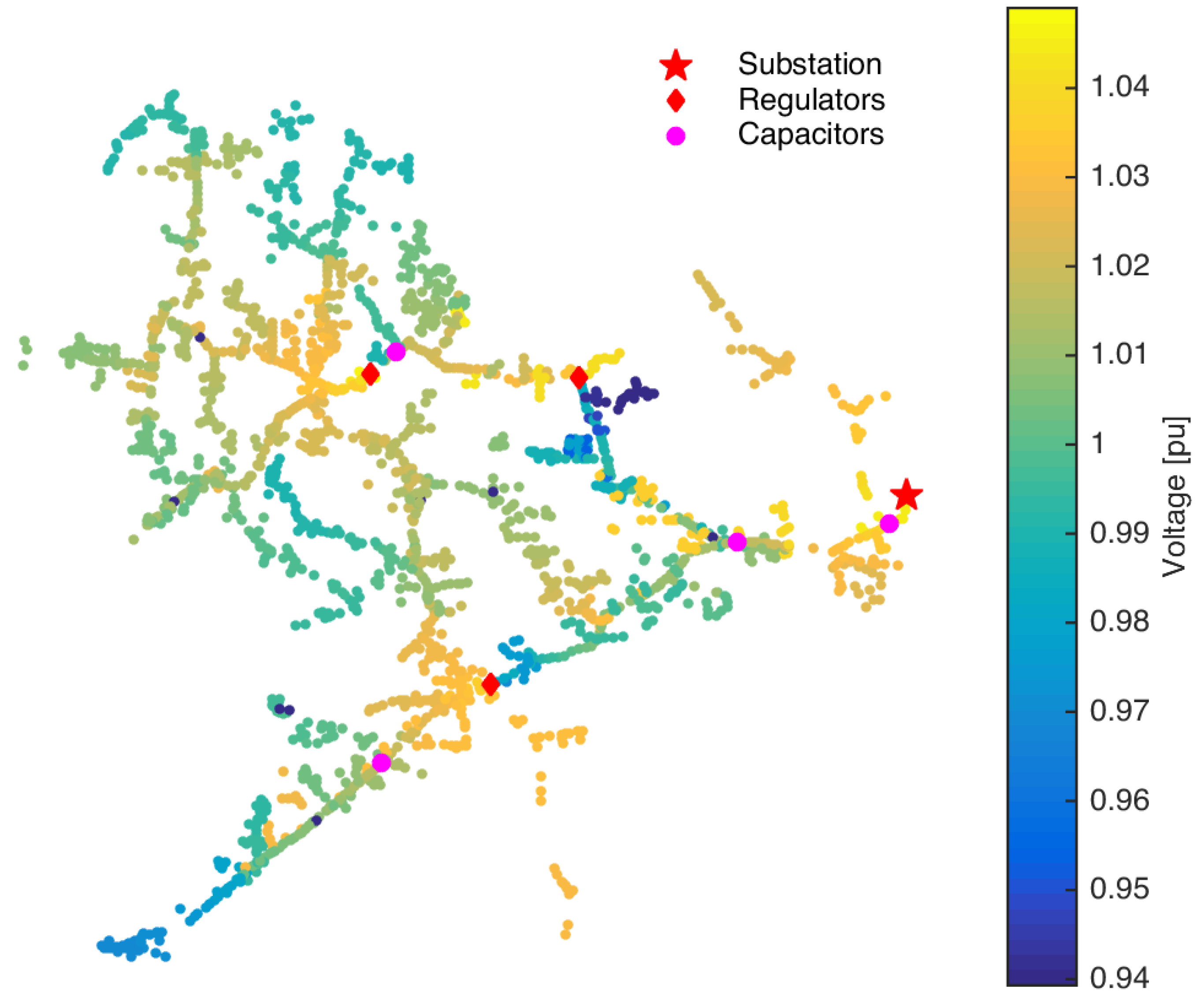
Figure 2.
Voltage profile for IEEE 8500 nodes test feeder. One phase per color, where continuous lines represent primary voltages and dashed lines represent secondary voltages.
Figure 2.
Voltage profile for IEEE 8500 nodes test feeder. One phase per color, where continuous lines represent primary voltages and dashed lines represent secondary voltages.

Figure 3.
Three-dimensional visualization for time-sequential simulation. Warmer colors represent higher voltage magnitudes.
Figure 3.
Three-dimensional visualization for time-sequential simulation. Warmer colors represent higher voltage magnitudes.
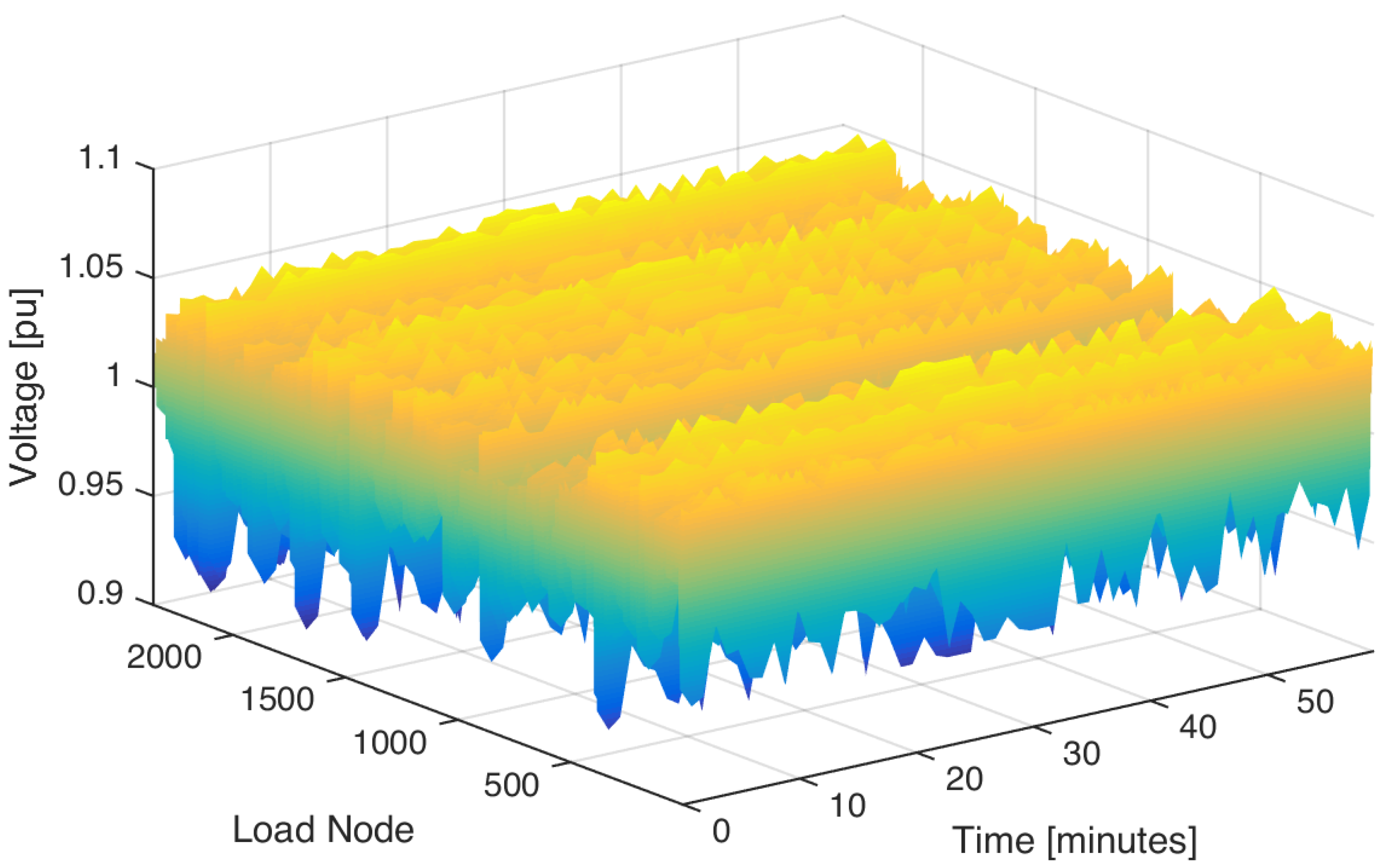
Figure 4.
Time-sequential simulation of 2354 loads. Each load line is associated with a different color.
Figure 4.
Time-sequential simulation of 2354 loads. Each load line is associated with a different color.

Figure 5.
Voltage magnitude (a) and geographical locations (b) for loads of interest in time-sequential simulation.
Figure 5.
Voltage magnitude (a) and geographical locations (b) for loads of interest in time-sequential simulation.

Figure 6.
Probabilistic distributions of load voltages.

Figure 7.
Density evolution of load voltages. Warmer colors represent higher statistical density.

Figure 8.
Contours for density evolution of load voltages with additional lines for voltage limits.


Table 1.
Review of validation strategies.
| Reference | Nodes | Electrical Simulation | Validation Variable | Visualization | ||||||
|---|---|---|---|---|---|---|---|---|---|---|
| Snapshot | Time-Sequential | Real-Time | V | I | P | Other | Figure | Table | ||
| [7] | 123 | ✓ | ✓ | ✓ | ✓ | ✓ | ||||
| [8] | 123 | ✓ | ✓ | ✓ | ✓ | ✓ | ✓ | |||
| [9] | 37 | ✓ | ✓ | ✓ | ✓ | ✓ | ✓ | ✓ | ||
| [10] | 8500 | ✓ | ✓ | ✓ | ✓ | ✓ | ||||
| [11] | 8500 | ✓ | ✓ | ✓ | ✓ | ✓ | ||||
| [12] | 8500 | ✓ | ✓ | ✓ | ✓ | ✓ | ||||
| [13] | 8500 | ✓ | ✓ | ✓ | ✓ | ✓ | ✓ | ✓ | ||
| [14] | 7000 a | ✓ | ✓ | ✓ | ✓ | ✓ | ✓ | ✓ | ||
| [15] | 200 a | ✓ | ✓ | ✓ | ✓ | ✓ | ||||
| [16] | 8500 | ✓ | ✓ | ✓ | ||||||
| [17] | 8500 | ✓ | ✓ | ✓ | ✓ | ✓ | ||||
| [18] | 8500 | ✓ | ✓ | ✓ | ✓ | ✓ | ||||
| [19] | 8500 | ✓ | ✓ | ✓ | ✓ | ✓ | ✓ | |||
| [20] | 738 | ✓ | ✓ | ✓ | ✓ | ✓ | ✓ | |||
| [21] | 9 a | ✓ | ✓ | ✓ | ✓ | ✓ | ✓ | |||
| [22] | 8500 | ✓ | ✓ | ✓ | ✓ | ✓ | ✓ | ✓ | ||
| [23] | 13 | ✓ | ✓ | ✓ | ✓ | ✓ | ✓ | ✓ | ||
| [24] | 400 | ✓ | ✓ | ✓ | ✓ | ✓ | ||||
| [25] | >200 a | ✓ | ✓ | ✓ | ✓ | |||||
| [26] | 15 | ✓ | ✓ | ✓ | ✓ | ✓ | ✓ | ✓ | ||
| [27] | 6999 | ✓ | ✓ | ✓ | ✓ | ✓ | ✓ | ✓ | ||
| [28] | 60 | ✓ | ✓ | ✓ | ✓ | ✓ | ✓ | ✓ | ||
| [29] | 8500 | ✓ | ✓ | ✓ | ✓ | ✓ | ||||
| [30] | 60 | ✓ | ✓ | ✓ | ✓ | ✓ | ||||
a Approximate count of calculated node voltages.
© 2017 by the authors. Licensee MDPI, Basel, Switzerland. This article is an open access article distributed under the terms and conditions of the Creative Commons Attribution (CC BY) license (http://creativecommons.org/licenses/by/4.0/).
Share and Cite
MDPI and ACS Style
Hernandez, M.; Ramos, G.; Padullaparti, H.V.; Santoso, S.
Statistical Inference for Visualization of Large Utility Power Distribution Systems
. Inventions 2017, 2, 11.
https://doi.org/10.3390/inventions2020011
AMA Style
Hernandez M, Ramos G, Padullaparti HV, Santoso S.
Statistical Inference for Visualization of Large Utility Power Distribution Systems
. Inventions. 2017; 2(2):11.
https://doi.org/10.3390/inventions2020011
Hernandez, Miguel, Gustavo Ramos, Harsha V. Padullaparti, and Surya Santoso.
2017. "Statistical Inference for Visualization of Large Utility Power Distribution Systems
" Inventions 2, no. 2: 11.
https://doi.org/10.3390/inventions2020011