Harnessing Deep Convolutional Neural Networks Detecting Synthetic Cannabinoids: A Hybrid Learning Strategy for Handling Class Imbalances in Limited Datasets

Abstract

The aim of this research was to develop and deploy efficient deep convolutional neural network (DCNN) frameworks for detecting and discriminating between various categories of designer drugs. These are of particular relevance in forensic contexts, aiding efforts to prevent and counter drug use and trafficking and supporting associated legal investigations. Our multinomial classification architectures, based on Attenuated Total Reflectance Fourier-Transform Infrared (ATR-FTIR) spectra, are primarily tailored to accurately identify synthetic cannabinoids. Within the scope of our dataset, they also adeptly detect other forensically significant drugs and misused prescription medications. The artificial intelligence (AI) models we developed use two platforms: our custom-designed, pre-trained Convolutional Autoencoder (CAE) and a structure derived from the Vision Transformer Trained on ImageNet Competition Data (ViT-B/32) model. In order to compare and refine our models, various loss functions (cross-entropy and focal loss) and optimization algorithms (Adaptive Moment Estimation, Stochastic Gradient Descent, Sign Stochastic Gradient Descent, and Root Mean Square Propagation) were tested and evaluated at differing learning rates. This study shows that innovative transfer learning methods, which integrate both unsupervised and supervised techniques with spectroscopic data pre-processing (ATR correction, normalization, smoothing) and present significant benefits. Their effectiveness in training AI systems on limited, imbalanced datasets is particularly notable. The strategic deployment of CAEs, complemented by data augmentation and synthetic sample generation using the Synthetic Minority Oversampling Technique (SMOTE) and class weights, effectively address the challenges posed by such datasets. The robustness and adaptability of our DCNN models are discussed, emphasizing their reliability and portability for real-world applications. Beyond their primary forensic utility, these systems demonstrate versatility, making them suitable for broader computer vision tasks, notably image classification and object detection.

1. Introduction

In today’s dynamic landscape, the proliferation of designer drugs, especially synthetic cannabinoids, has emerged as a significant risk to global health and security. The rapid escalation of these substances presents a formidable challenge to law enforcement, forensic, and public health institutions due to their structural diversity and the ceaseless emergence of new variants. As a result, there is an urgent need within the scientific community and relevant institutions to develop robust tools and methodologies, enabling fast and reliable detection and screening of these compounds.

Infrared (IR) spectroscopy, with a particular emphasis on the Attenuated Total Reflectance Fourier-Transform Infrared (ATR-FTIR) technique, offers numerous advantages in detecting and identifying substances of abuse over other spectroscopic methods. Attributes like minimal sample preparation, rapid analysis, non-destructive testing, adaptability to field testing, high sensitivity and selectivity, and compatibility with spectral databases position it as an invaluable tool for law enforcement, forensic analysis, and other contexts requiring swift and reliable identification of illicit substances [1].

Nevertheless, the extensive variety and evolving structures of synthetic cannabinoids result in intricate spectral signatures, rendering traditional analysis methods insufficient. To address this issue, contemporary research is gravitating toward artificial intelligence (AI), specifically deep learning (DL), to enhance the accuracy and efficiency of drug identification using ATR-FTIR spectra [2,3].

Deep convolutional neural network (DCNN) models are specifically tailored for image processing and computer vision tasks because of their inherent ability to process spatial hierarchies in data. Convolutional Autoencoders (CAEs) are a variant of the standard autoencoder and incorporate convolutional layers instead of fully connected layers. This makes them particularly suitable for dimensionality reduction and representation learning in a variety of tasks. The convolutional layers allow these autoencoders to exploit the spatial hierarchies and structures in image data, making them more efficient at encoding image-specific patterns. Transformers, initially introduced for natural language processing tasks, use self-attention mechanisms to assign different weights to input features. This way, they yield state-of-the-art results across a variety of NLP tasks [4,5,6,7,8,9,10,11,12,13].

Our research is part of ongoing efforts addressing the growing challenges of synthetic drug proliferation. In a prior study, we obtained promising results with a DCNN model based on the adapted Inception-V3 architecture [14]. In this work, we have presented the performances of a custom-designed DCNN, which was developed from scratch and combined with a specially designed pre-trained Convolutional Autoencoder. Additionally, we presented a new model derived from the vision transformer trained on ImageNet competition data (ViT-B/32) from The Wolfram Neural Net Repository [15,16,17]. We developed and refined these architectures using the Wolfram Mathematica v. 13.2 and Python v. 3.11.5. programming platforms. Each model offers unique features, making them suitable for diverse image processing tasks [18,19].

The DCNN system, grounded in the foundation provided by the pre-trained structure of the vision transformer trained on ImageNet competition data (ViT-B/32), stands as a pioneering study. It is the first architecture explicitly tailored for the detection and classification of synthetic cannabinoids. Notably, this marks the inaugural utilization of the vision transformer family within the specialized realm of forensic designer drug detection and screening.

The outcomes from these models underscore the effectiveness of deep learning and transfer learning methodologies in addressing the intricate challenge of designer drugs in the pivotal domain of forensic science. Their inherent portability allows for facile in situ deployment, and their versatility suggests potential adaptability to non-forensic tasks, specifically within image classification and object detection areas of computer vision.

2. Materials and Methods

2.1. Related Work

The application of artificial intelligence (AI) for the detection of designer drugs, especially when combined with instruments like ATR-FTIR spectrometers, has seen impressive growth over the last decades. This surge has facilitated enhanced methodologies in drug discovery and efforts to curtail drug use and trafficking and support relevant legal investigations.

Pereira et al. devised a new supervised classification method that incorporated Partial Least Squares Discriminant Analysis (PLS-DA) and ATR-FTIR to pinpoint New Psychoactive Substances (NPS) in blotter papers, as well as a presumptive method for identifying drugs in seized ecstasy tablets [20,21]. Another recent study used six machine learning models—including K-Nearest Neighbor (KNN), Support Vector Machine (SVM), Random Forest (RF), Extra Trees (ETs), voting, and Artificial Neural Networks (ANNs)—to categorize eight different categories of designer drugs including synthetic cannabinoids, synthetic cathinones, phenethylamines, fentanyl analogs, and other substances based on the IR spectral data acquired from various FTIR spectrometers [22]. Another study introduced a portable near-infrared spectrometer for the tentative identification of psychotropic drugs through library searching and mathematical pretreatment methods [23].

Convolutional Neural Networks (CNNs) have made significant strides in image analysis. Their utility was demonstrated in studies that classified immunohistochemical images of different tumor cell lines, distinguishing between normal and tumorous lines. Such approaches can potentially be instrumental in drug discovery and the identification of misused prescription medications [24].

Obtaining sufficiently large datasets and determining optimal hyperparameters remain challenges in AI-based drug analysis [25]. The efficiency of the validating techniques is crucial to determining their enhancement capabilities, especially in Quantitative Structure-Activity Relationship (QSAR) analyses examining drug–protein interactions, as illustrated in Mendenhall and Meiler’s research [26].

Yet, amid these challenges, several innovations have surfaced. DCNNs have been tailored for predicting the bioactivity of small molecules in drug discovery, and Encoder–Decoder Deep Neural Networks (DNNs) have been used for target-based drug design [27,28]. Autoencoders, especially the denoising variant, were found to be very effective in various applications predicting drug–target interactions, with Convolutional Autoencoders (CAEs) in image processing emerging as a frontier in deep learning [29,30].

Large deep learning models encompassing a myriad of CNN architectures, like VGG, DenseNet, MobileNet, ResNet, and Google’s Inception, dominate image classification applications [31,32,33,34,35]. These networks typically act as pre-trained feature extractors, with their knowledge subsequently transferred to specialized smaller networks to address specific image classification challenges.

Transformers, originally proposed for machine translation tasks by Vaswani et al., have been refined and employed extensively in various natural language processing (NLP) applications [10,36]. The introduction of the vision transformer (ViT) system has revolutionized image recognition tasks by offering a compelling alternative to CNNs in terms of computational efficiency and accuracy [37].

Our study contributes to the growing body of literature that delves into image recognition, specifically targeting small to medium scales within imbalanced datasets. We employed artificial intelligence tools rooted in hybrid transfer learning methodologies that seamlessly integrate both supervised and unsupervised techniques.

Aiming for reliability and accuracy, our DCNN architectures have incorporated a minimal Convolutional Autoencoder model that we created and pre-trained, as well as a tailored structure derived from a pre-trained model within the vision transformer family. The most distinctive feature of our proposed approach compared to other state-of-the-art criminological methodologies is rooted in the unique training strategy that was used for the CAE. Initially, our CAE was pre-trained on a larger dataset of unlabeled non-forensic spectral images. This foundational training facilitates the CAE to better recognize inherent ATR-FTIR patterns, priming it for more efficient subsequent training in identifying broader specific chemical structures in spectral images. Once this foundational learning is solidified, we froze the layers of the CAE to retain these discerned spectral patterns. Following the addition of classification block layers, the resulting DCNN system underwent training, validation, and testing on datasets of labeled investigative spectral images. The process culminated in a decisive fine-tuning of the target substance group. This multi-stage, specialized training approach proved remarkable efficiency in the system, especially in scenarios where forensic datasets are both limited and imbalanced.

The primary application domain for the AI systems we developed is the detection and class recognition of synthetic cannabinoids, especially JWH synthetic cannabinoids, which is an under-explored area that often overlooks the issue of emerging drugs of abuse. In addition, we sought to ensure the portability and versatility of the networks we crafted for potential broader applications in non-forensic areas under the computer vision category. In designing our models, we closely adhered to simplicity, keeping the architecture as straightforward as possible (refer to Figure 1). One significant advantage of this intentionally uncomplicated setup is the ability to utilize scalable DCNN architectures—along with their efficient implementations—with minimal adjustments.

We combined methods of spectral image preprocessing, such as ATR correction, normalization and smoothing, complemented by data augmentation and synthetic sample generation using the Synthetic Minority Oversampling Technique (SMOTE) and class weights. We leveraged various loss functions, including cross-entropy and focal loss, and various optimization algorithms applied at various learning rates.

The outcomes from our investigative experiments underscore the remarkable accuracy and efficiency of the systems we designed. Notably, in the segment pertaining to synthetic cannabinoids, our method demonstrates outstanding accuracy. As we pivoted our attention to non-forensic target domains, such as image classification and object detection, our approach consistently aligned with the top-tier systems documented in the research literature [38,39,40,41,42,43].

2.2. Computational Platform

In the computational experiments documented herein, we utilized standalone, non-clustered Dell G15 5520 platforms equipped with a 12th Gen Intel^® Core™ i7-12700H processor boasting 14 cores, 20 threads, and operating at up to 4.540 GHz with Turbo Boost technology. Every machine had 32 GB of RAM, integrated Intel Iris Xe Graphics, and an additional 6 GB GDDR6 NVIDIA GeForce RTX 3060 Graphics Unit. It ran on the Windows 11 Pro operating system and Linux Ubuntu Server 23.04.

For the preliminary assessment of our computational framework, we carried out a series of benchmark tests using the High-Performance Linpack (HPL) implementations and the Intel^® Distribution for LINPACK* Benchmark, a front-end console based on modifications and additions to the HPL from Innovative Computing Laboratories at the University of Tennessee, Knoxville [44]. The Linpack Benchmark test is a measure of a computer’s floating-point rate of execution. It is determined by running a computer program that solves a dense system of linear equations. It was originally intended to give users of the package a feeling of how long it would take to solve certain matrix problems. The benchmark was stated as an appendix to the Linpack Users’ Guide and has grown since it was published in 1979 [45,46].

It addresses the solution of a dense system (real*8) of linear equations (denoted as Ax = b) employing double-precision arithmetic. It quantifies the time required for both factorization and system resolution, subsequently translating this duration into a performance metric. The solution’s precision is then assessed. Importantly, Linpack Benchmark allows for a flexible number of equations (N) to be solved, with no inherent limitation set at 1000. The implementation incorporates partial pivoting to ensure result reliability. The parameters and results of the Intel^® Distribution for LINPACK* Benchmark are highlighted in

Table 1. Parameters of the Intel^® Distribution for LINPACK* Benchmark.

Tests	Number of Equations to Solve (Problem Size)	Leading Dimension of Array (LDA)	Number of Trials to Run	Data Alignment Value (in Kbytes)
1	1000	1000	8	4
2	2000	2000	6	4
3	5000	5008	4	4
4	10,000	10,000	4	4
5	15,000	15,000	3	4
6	18,000	18,008	3	4
7	20,000	20,016	3	4
8	22,000	22,008	3	4
9	25,000	25,000	3	4
10	26,000	26,000	3	4
11	27,000	27,000	2	4
12	30,000	30,000	1	1
13	35,000	35,000	1	1
14	40,000	40,000	1	1
15	45,000	45,000	1	1

and

Table 2. Results obtained with the Intel^® Distribution for LINPACK* Benchmark.

Floating Point Operations per Second Average (GFlop/s)
Test	Average	Maximal	Residual	Residual Norm	Check
1	173.7785	202.8784	1.30 × 10−6	3.94 × 10−4	pass
2	229.6025	253.6362	1.30 × 10−6	3.94 × 10−4	pass
3	276.6376	293.3389	1.30 × 10−6	3.94 × 10−4	pass
4	270.1227	275.2453	1.30 × 10−6	3.94 × 10−4	pass
5	254.1475	258.5500	1.30 × 10−6	3.94 × 10−4	pass
6	253.9643	255.3168	1.30 × 10−6	3.94 × 10−4	pass
7	259.4283	261.4543	1.30 × 10−6	3.94 × 10−4	pass
8	253.8448	256.6712	1.30 × 10−6	3.94 × 10−4	pass
9	256.9164	257.9535	4.17 × 10−6	3.29 × 10−4	pass
10	255.6003	259.7284	4.17 × 10−6	3.29 × 10−4	pass
11	258.8156	313.4706	4.17 × 10−6	3.29 × 10−4	pass
12	255.3485	255.3485	4.17 × 10−6	3.29 × 10−4	pass
13	254.7538	254.7538	4.17 × 10−6	3.29 × 10−4	pass
14	257.2128	312.2128	4.17 × 10−6	3.29 × 10−4	pass
15	133.0238	133.0238	2.33 × 10−5	3.07 × 10−4	pass

.

The results collectively offer insights into the computational performance and accuracy of our systems when solving large systems of linear equations. This information is valuable for assessing the suitability of a computing environment for scientific and engineering simulations [47].

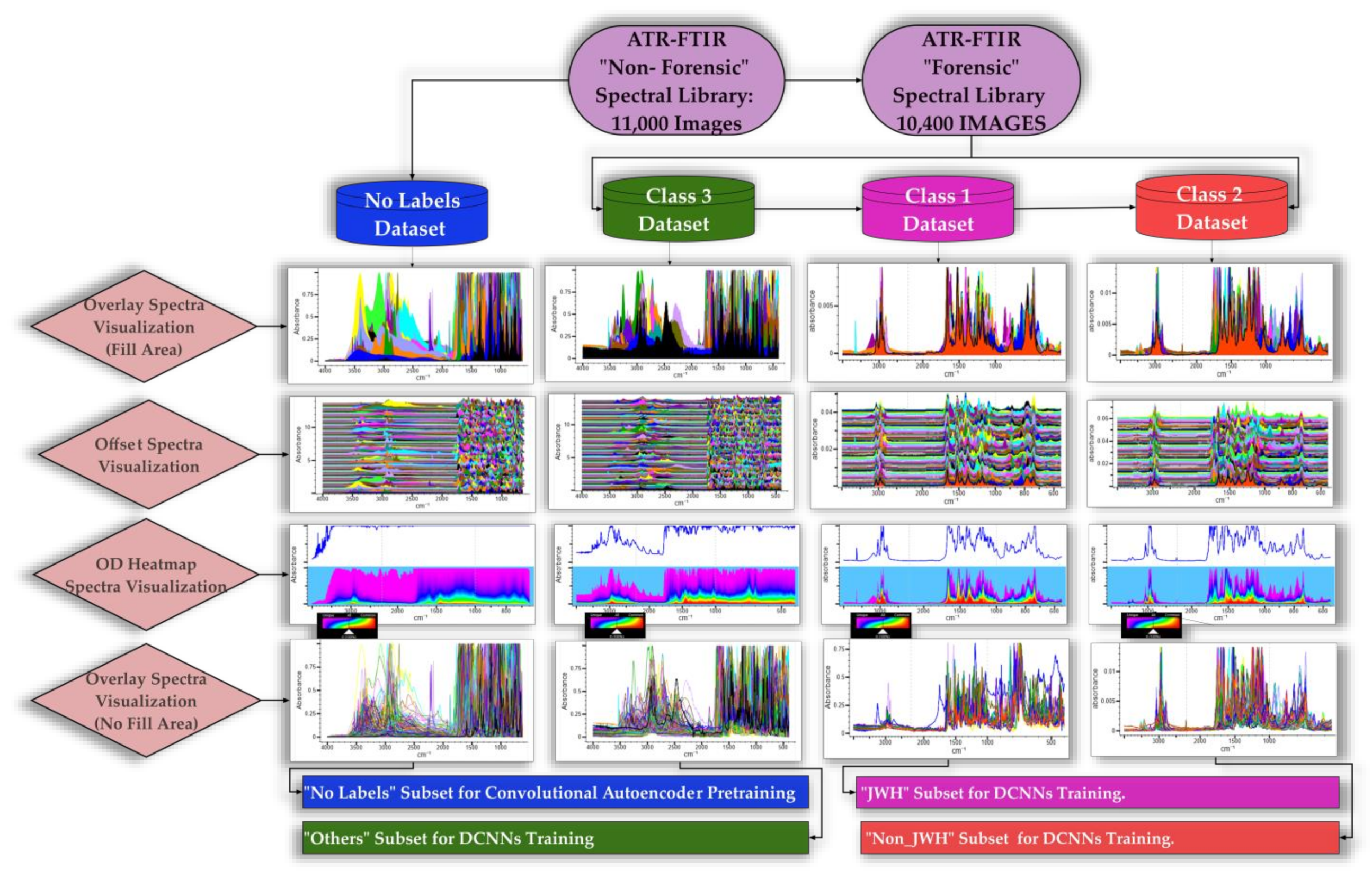
2.3. The Spectral Database

The ATR-FTIR spectra used in this research are sourced from our proprietary database pyDETECT-FTIR DATABASE, which includes both experimentally acquired data and information retrieved from public, open-access spectral libraries. Each sample housed in our database has undergone external and independent validation through appropriate analytical methods.

The spectral data were predominantly acquired through ATR-FTIR spectroscopy, complemented occasionally using ATR-Neat and ATR-Film techniques. A significant proportion of the abuse-prone substance spectra were procured using a Nicolet iN10 MX spectrometer. Subsequent to the pre-processing and analytical processing phases, all spectral files pertaining to the synthetic drugs of abuse used in the investigation were transformed into monochromatic spectral images (.bmp format), encoded suitably, and subsequently integrated within the enriched datasets served as the foundational elements in the conceptualization, training, and refinement of DCNNs.

From this extensive data repository, we curated two pivotal spectral libraries: the Non-Forensic ATR-FTIR Spectral Library, encompassing 11,000 images earmarked for CAE pre-training, and a pertinent Forensic ATR-FTIR Spectral Library, collectively housing 10,425 images, designated for the comprehensive training and fine-tuning of the DCNN models.

To enhance the training and fine-tuning of our DCNN models, we used spectral imagery from the Forensic ATR-FTIR Spectral Library, which was partitioned into three unique categories representing various substances of abuse.

• Class 1 comprises 125 images of JWH synthetic cannabinoids (which were first synthesized by Dr. John W. Huffman), falling into 11 structural subclasses such as Naphthoylindoles (e.g., JWH-018, JWH-073); Alkylated Naphthoylindoles (e.g., JWH-122 8-Methylnaphthyl isomer, JWH-018 2’-Naphthyl isomer); Cyclohexylphenols (e.g., JWH-015, JWH-133); Fluorinated Naphthoylindoles (e.g., FUB-JWH-018, JWH-210 N-[5-Fluoropentyl] analog); Hydroxylated Naphthoylindoles (e.g., JWH-018-4, JWH-019 N-[6-Hydroxyhexyl] metabolite); Chlorinated Naphthoylindoles (e.g., JWH-398 6-Chloronaphthyl isomer, JWH-398 2-Chloronaphthyl isomer); Benzoylindoles (e.g., JWH-302, JWH-307); Phenylacetylindoles (e.g., JWH-250, JWH-251); Naphthylmethylindenes (e.g., JWH-081, JWH-210); Adamantoylindoles (e.g., JWH-018 Adamantyl analog, JWH-018 Adamantyl carboxamide); and Naphthoylpyrroles (e.g., JWH-147, JWH-370).
• Class 2 houses 250 images of non-JWH synthetic cannabinoids, covering several distinct groups such as Classical Cannabinoids (e.g., HU-210, synthesized by Dr. Raphael Mechoulam and his colleagues from Hebrew University, Tetrahydrocannabinol, Cannabidiol, Cannabinol, Cannabichromene, Cannabigerol); Hybrid Cannabinoids (e.g., AM 251 developed by Alexandros Makriyannis at Northeastern University, URB-447 from the University of Rome “La Sapienza Biomedical”); Aminoalkylindoles (e.g., WIN 55,212-2, RCS-8, CHMINACA, Cumyl-PICA, APINACA); Aminoalkylindazoles (e.g., AB-FUBINACA, AB-PINACA), etc.
• Class 3 encompasses a broad spectrum of other designer drugs, totaling 10,050 images. This third heterogeneous class, substantial in its diversity, not only broadens the classification spectrum but also enhances the comparative dimension of the machine learning process. These originate mainly from categories such as psychedelics, piperazines, dissociatives, empathogens, stimulants, sedatives, abused prescription medications, and other drugs of similar importance (e.g., Lysergic Acid Alpha-Hydroxy-Ethylamide, α-Ethyltryptamine, Scaline, 25B-NBOMe, 25C-NBOH, Fentanyl-Furanyl, Testosterone, Flubromazepam, Cocaine, Diazepam, Heroin, Morphine, Scopolamine, Strychnine, Pheniramine, etc.).

The present scientific research will continue in the future with the development of other types of artificial intelligence systems for the detection and recognition of synthetic cannabinoids. Moreover, the implementation of the already designed systems is also planned. An exhaustive list of representative synthetic cannabinoids used for this study will be available upon the completion of the research. Some of the synthetic cannabinoids used have been documented in a previous paper. [48].

The detection of synthetic cannabinoids, specifically of the JWH and non-JWH cannabinoids categories, presented a challenge due to the significant class imbalance observed within our datasets. The class imbalance could potentially bias the DCNN classification models toward the majority class, thereby undermining the predictive accuracy for the minority classes that are of main interest in this study. To address this issue, several strategies were adopted to enhance the performance of our DCNN model. These strategies are outlined below.

To counter the effect of class imbalance, we adjusted the loss function to incorporate class weights. This involved calculating the loss separately for each class and then multiplying it with the respective class weight before aggregating them to obtain the final loss. This adjustment helps in penalizing misclassifications of the minority class more heavily compared to the majority class.

The loss function was modified to include a weighted term that depends on the class distribution. For instance, if class 1 has 125 samples and class 2 has 250 samples, the weights could be computed as the inverse of the number of samples in each class, and then normalized to sum up to one.

Each variety of the spectral library is illustrated in Figure 2 through respective visualizations including overlay spectra (fill area), offset spectra, overlap density heatmap spectra, and overlay spectra (no fill area).

Using the 5-fold cross-validation method, the datasets were partitioned into training, validation, and test subsets, adhering to a conventional distribution of 60% for training and 20% each for validation and testing purposes. A detailed enumeration of the number of images allocated for training, validation, and testing across all three datasets is delineated in

Table 3. Number of training, validation, and testing images included in the datasets.

Spectral Library	Training Set	Validation Set	Test Set
Non-Forensic	6600	2200	2200
Forensic	6255	2085	2085

.

Oversampling is a technique used to augment a minority class either by duplicating existing samples or by creating synthetic samples.

• Duplicating Existing Samples: involves replicating some of the minority class instances to balance the class distribution;
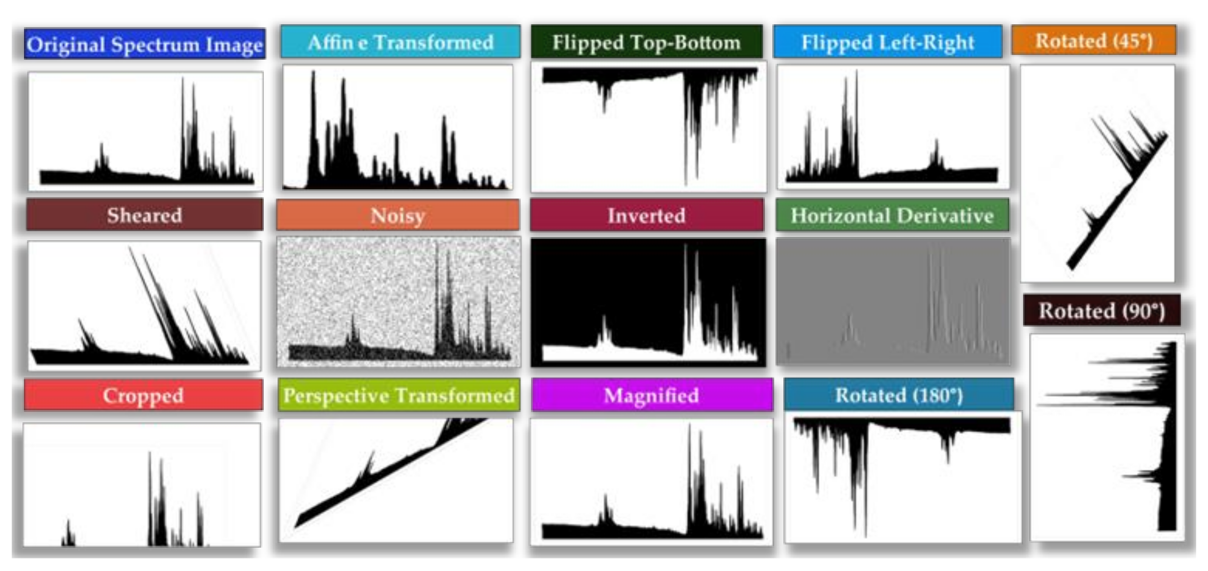
• Data Augmentation: involves augmenting the data through techniques, such as random rotations, shifts, and zooms, in order to generate additional synthetic samples.

The Synthetic Minority Oversampling Technique (SMOTE) is a statistical technique that we used to augment the number of instances in the minority class(es) of our dataset. The module works by generating new instances from existing minority cases that are supplied as inputs. This is achieved by synthesizing new examples from the minority class. We have applied SMOTE on the feature space where new samples were generated through interpolation between existing minority class samples. This technique was particularly used to enhance the representation of the classes of JWH and non-JWH cannabinoids in the dataset [49].

Class weights are a set of coefficient values that are applied to the loss function during the training phase. These weights give more importance to the minority class, thus compensating for the imbalance. In our case, different weights were assigned to classes in the loss function to counterbalance the inequity in the dataset. The weights were assigned based on the inverse frequency of the classes. First, we determined the weights for each class based on the number of samples in each class. A common way to do this is using the following formula:

weight_class_i = total_samples/num_classes × num_samples_class_i.

In our case:

• Total number of samples (total_samples) = 125 + 250 + 10,050 = 10,425;
• Number of classes (num_classes) = 3.

The number of samples in each class was:

• Class 1 (JWH): 125;
• Class 2 (non-JWH): 250;
• Class 3 (other designer drugs): 10,050.

The weights for each class would thus be calculated as:

• weight_class_1 = 10,425/3 × 125 ≈ 27.80;
• weight_class_2 = 10,425/3 × 250 ≈ 13.90;
• weight_class_3 = 10,425/3 × 10,425 ≈ 0.33.

To implement this in the Wolfram Mathematica programming platform, we adopted a distinct strategy, given that the platform does not possess built-in support for class weights during training, as is the case with Keras. Nonetheless, we manually modified the loss function to incorporate the weights. This entailed calculating the loss separately for each class, followed by multiplying it by the respective class weight prior to aggregating them to derive the final loss.

The OpenChrom Lablicate Edition v. 1.5.0 and Spectragryph v. 1.2.16.1 software packages facilitated the meticulous handling and processing of spectra, enhancing their visual representation for more robust analysis and comparison, as well as rectifying potential spectral discrepancies [50,51]. Our exploration encompassed some of the spectral processing techniques, with the three most pivotal methods illustrated in Figure 3.

ATR correction made the ATR spectra look more like a transmission spectrum. Normalization set the minimum and maximum points to particular values for scaling a spectrum. All spectra used in our scientific approach were normalized to the value of 1. Smoothing reduced the noise in a spectrum. To smooth all spectra, we selected the algorithm according to the characteristics of each, setting the following parameters: quad-cubic Savitzky–Golay; number of points: 5; and Fourier strength: 80%.

Data augmentation is a common practice in ML, particularly in the field of computer vision, where the aim is to increase the amount and diversity of data without actually collecting new data [52,53]. In the context of our research project, data augmentation was used to artificially increase the number of images of IR spectra used for training the DCNN models. The concept behind data augmentation is simple but powerful. By applying a series of random but realistic transformations to the input images, such as rotations, shifts, flips, zooms, and more, we created a broader set of data for the model to learn from. This helps the model generalize better and reduces the risk of overfitting, especially when dealing with a limited number of original samples.

In our case, the original set of spectral images was artificially expanded during training. The exact number of images created depended on the augmentation strategies that we used. Typically, these transformations are applied on the fly during the training process, which means that the augmented images are not physically saved in our storage but are generated dynamically in each epoch.

This approach allows the models to see slightly different variations of the spectra in each iteration, thereby enriching the diversity of training data without consuming extra storage space (Figure 4). Further research is underway to explore other potential strategies, such as data synthesis using Generative Adversarial Networks (GANs) and hybrid techniques that combine oversampling with undersampling the majority class, to create a more robust and unbiased DCNN model for the classification of synthetic cannabinoids [54,55].

2.4. Core Components of the Developed DCNNs

The fundamental operations performed for building our DCCNs were encompassed by the basic operation modules, i.e., convolution, pooling, and full connection.

• Convolution (Convolution Layers)

Convolution is a mathematical operation that involves sliding a filter (often referred to as a kernel) over the input data (such as an image) to produce a feature map or convolved output. Specifically, for each position of the filter on the input, the convolution operation computes the element-wise product between the filter and the portion of the input it covers, followed by a sum of all those products. This operation allows the network to learn spatial hierarchies and extract local features, making DCNNs particularly well-suited for tasks, such as image recognition.

The equation used for convolution is:

$$(\mathrm{I}\times \mathrm{K})(\mathrm{x},\mathrm{y})={\sum }_{\mathrm{i}=-\mathrm{\infty }}^{\mathrm{\infty }}{\sum }_{\mathrm{j}=-\mathrm{\infty }}^{\mathrm{\infty }}\mathrm{I}(\mathrm{i},\mathrm{j})\times \mathrm{K}(\mathrm{x}-\mathrm{i},\mathrm{y}-\mathrm{j}),$$

(1)

where I is the input image, K is the convolutional filter or kernel, and x and y are the coordinates of the current pixel.

Contrary to the general equation of convolution, which considers infinite summations, in a DCNN, the summation only occurs over the dimensions of the filter, which are typically small and finite (e.g., 3 × 3 or 5 × 5).

b.

Pooling (Pooling Layers)

Pooling is used to downsample the spatial dimensions of a feature map, thereby reducing the computational cost for subsequent layers and helping to make the network invariant to small translations. There are various types of pooling operations, with max pooling and average pooling being the most common.

In max pooling, for each segment of the feature map covered by the pooling window (often 2 × 2 or 3 × 3), only the maximum value within that segment is retained in the output feature map. In average pooling, the average value of all the numbers within the pooling window is taken and used in the output feature map. Given a feature map M, the max pooling operation for a 2 × 2 window at position (i, j) can be represented for max pooling as:

P(i, j) = max{M(i, j),M(i + 1, j),M(i, j + 1),M(i + 1, j + 1)},

(2)

and for average pooling, for the same 2 × 2 window:

P(i, j) = max{M(i, j),M(i + 1, j),M(i, j + 1),M(i + 1, j + 1)},

(3)

where P(i, j) is the output of the pooling operation at position (i, j), M is the input feature map, and i, j is the position coordinates in the feature map.

c.

Full Connection (Fully Connected Layer)

A fully connected layer connects every neuron (or node) from one layer to every neuron of the next layer. It is primarily used to flatten the output from the convolutional layers and combine extracted features, eventually leading to the final output of the network, such as a classification result. Given an input vector x and weights W, the output y of the fully connected layer is computed.

The equation for the fully connected layer is:

y = W ∗ x + b,

(4)

where y is the output vector of the fully connected layer, x is the input vector to the fully connected layer, W is the weight matrix associated with the layer, and b is the bias vector for the layer.

2.5. Loss Functions, Activation Algorithms, Optimization, Regularization, and Fine-Tuning in the Developed DCNNs

In order to assess and refine our models, we explored the loss functions of cross-entropy and focal loss. Additionally, we tested various optimization techniques, such as Adaptive Moment Estimation (ADAM), Stochastic Gradient Descent (SGD), Sign Stochastic Gradient Descent (Sign SGD), and Root Mean Square Propagation (RMS Prop), all at diverse learning rates.

d.

Focal Loss Function

After extensively evaluating various loss functions for our DCNNs, we found that the focal loss demonstrated the best performance, particularly for our class imbalance scenario. Introduced to address the class imbalance problem in object detection, focal loss was designed to focus on misclassified instances, ensuring that well-classified instances do not dominate the training.

During the experiments, it became evident that focal loss consistently yielded superior results, improving the sensitivity of the model to the less frequent classes. The modulating factor introduced by focal loss downweighted the contribution of easy examples, allowing our DCNNs to focus on the hard-to-classify instances. This was instrumental in achieving a balance between the precision and recall for all classes, irrespective of their frequency.

Given the marked improvements in classification performance, combined with its inherent ability to handle class imbalance, we elected to retain focal loss as our primary loss function for the DCNN models. The results not only validated our decision but reinforced the potential of focal loss in scenarios where class distribution is skewed.

The focal loss is an enhanced version of the cross-entropy loss, introduced to handle class imbalance. The focal loss downweighs the contribution of easy examples and focuses more on the hard ones, thus the name focal [56]. The focal loss is defined based on the true class label y (which is either 0 or 1 for binary classification or a one-hot encoded vector for multi-class classification), the predicted probability p of the data point belonging to the positive class, the focusing parameter γ (which adjusts the rate at which easy examples are downweighted; when γ = 0, the focal loss is equivalent to cross-entropy), and a weighting factor α in the range to balance the importance of positive/negative classes.

The α factor is set to 1 for the positive class and 0 for the negative class in the binary case. For multi-class classification, α can be extended to be a vector rather than a scalar. Each element in the α vector corresponds to a class. The sum of all elements in the α vector is typically 1, but this is not a strict requirement. The values just need to provide the desired balance among the classes. For a three-class problem, we have α₁ for Class 1, α₂ for Class 2, and α₃ for Class 3.

When we considered Class 1 (JWH) as the smallest, Class 2 (non_JWH) as intermediate, and Class 3 (others) as the largest class, we assigned a higher α value to Class 1 to give it more weight in the loss calculation. We gave a moderate α value to Class 2 and the smallest α value to Class 3. Our intention in choosing these α values was to balance out the contribution of each class to the loss, especially when there was a class imbalance.

We denoted the proportion of each class as p₁, p₂, and p₃. A common approach that we also used is to set α inversely proportional to the class sizes:

$$\mathsf{\alpha }1=\frac{1}{\mathrm{p}1};\mathsf{\alpha }2=\frac{1}{\mathrm{p}2};\mathsf{\alpha }3=\frac{1}{\mathrm{p}3},$$

(5)

Next, we normalized the α values, so they summed up to 1:

Normalization factor = α1 + α2 + α3,

(6)

$$\mathsf{\alpha }1=\frac{\mathsf{\alpha }1}{\mathrm{Normalization}\mathrm{factor}},$$

(7)

$$\mathsf{\alpha }2=\frac{\mathsf{\alpha }2}{\mathrm{Normalization}\mathrm{factor}},$$

(8)

$$\mathsf{\alpha }3=\frac{\mathsf{\alpha }3}{\mathrm{Normalization}\mathrm{factor}}.$$

(9)

By setting the α values in this manner, we were effectively giving more importance to misclassifying an example from the smallest class and less importance to misclassifying an example from the largest class. This strategy helped us mitigate the impact of class imbalance during training.

The focal loss for a DCNN with 3 classes is defined as:

$$\mathrm{FL}(\mathrm{y},\mathrm{p})=-{\sum }_{\mathrm{i}=1}^3\mathsf{\alpha }\mathrm{i}(1-\mathrm{pi})\mathsf{\gamma }\mathrm{i}\log \left(\mathrm{pi}\right)$$

(10)

where pi is the predicted probability for the data point belonging to class i, yi is 1 if the data point belongs to class i and 0 otherwise, and αi is the weight of class i.

e.

Activation Algorithms

Upon evaluating various activation functions for our DCNNs, including the Rectified Linear Unit (ReLU), Sigmoid, Hyperbolic Tangent, and Softmax, we found ReLU to be the most effective for hidden layers due to its rapid convergence and computational efficiency.

However, for the output layer, especially in multi-class classification tasks, Softmax was retained for its ability to provide probability distributions over the classes. While other functions had their merits, the balance of speed and performance of the ReLU was unmatched by the other algorithms for the hidden layers of our DCNNs. Its capability to pass positive values and clip negatives to zero introduced non-linearity without complexity. Thus, the combination of the ReLU for hidden layers and Softmax for the output layer was pivotal in achieving the robust and accurate network performance obtained for our DCNNs.

f.

Rectified Linear Unit (ReLU)

The ReLU is a type of activation function that is widely used in convolutional neural networks and deep learning models. The function itself is quite simple and is defined as:

$$\mathrm{f}\left(\mathrm{x}\right)=\max (0,\mathrm{x})$$

(11)

This means that the function returns x if x is greater than or equal to zero and returns zero otherwise. In more intuitive terms, the ReLU function allows positive values to pass through unchanged while setting all negative values to zero. This non-linearity, while simple, has been found to work well in practice and has the benefit of being computationally efficient.

g.

Softmax

Softmax is an activation function primarily used in the output layer of a neural network, especially in multi-class classification tasks. It takes a vector of arbitrary real-valued scores (often called logits) and squashes it to a vector of values between zero and one that sums to one. The output values can be interpreted as probabilities of respective classes. It is often used in the output layer of a classifier to represent probability distributions over K classes:

$$\mathsf{\sigma }\left(\mathrm{z}\right)\mathrm{j}=\frac{{\mathrm{e}}^{\mathrm{z}}\mathrm{j}}{{\sum }_{\mathrm{k}=1}^{\mathrm{K}}{\mathrm{e}}^2\mathrm{k}}$$

(12)

For j = 1, …, K. In this equation, σ(z)i represents the probability of the ith class given the input vector z, z_i is the input logit for the i th class, K represents the total number of classes, and e is the base of natural logarithms.

h.

Optimization techniques

We undertook extensive experimentation with a variety of optimization algorithms such as ADAM, SGD, Sign SGD, and RMS Prop. Among them, the ADAM algorithm emerged as the standout performer. The successes of ADAM can be attributed to its unique combination of momentum and RMSprop techniques [57]. This dual approach enabled our network to benefit from both the accelerated convergence of momentum and the adaptive learning rates of RMSprop. Such a combination not only provided a boost in terms of the speed of convergence but also ensured stability during training.

A notable feature that worked in our favor was the inherent bias correction mechanism of ADAM. It ensured that even in the early stages of training when estimates can be considerably biased, the model was safeguarded against erratic behaviors. The hyperparameters provided by ADAM, especially the learning rate, were fine-tuned to our specific problem, further amplifying its effectiveness.

i.

ADAM optimization algorithm

The fundamental idea behind ADAM is to compute adaptive learning rates for each parameter by considering the first and second moments of the gradients. The equations for the ADAM update rule considering our context were:

• Compute the gradient gt of the focal loss for the three-class problem at step t.
• Update the moment estimates:

mt = β₁ × m_t−1 + (1 − β₁) × gt,

(13)

vt = β₂ × v_t−1 + (1 − β₂) × gt²,

(14)

3.

Correct bias in moment estimates:

$${\widehat{\mathrm{m}}}_{\mathrm{t}}=\frac{\mathrm{mt}}{{1-\mathsf{\beta }1}^{\mathrm{t}}}$$

(15)

$${\widehat{\mathrm{v}}}_{\mathrm{t}}=\frac{\mathrm{vt}}{{1-\mathsf{\beta }2}^{\mathrm{t}}}$$

(16)

4.

Update the parameters of the DCNN:

$$\mathsf{\theta }\mathrm{t}=\mathsf{\theta }\mathrm{t}-1-\mathsf{\alpha }.\frac{\widehat{\mathrm{m}}\mathrm{t}}{\sqrt{\widehat{\mathrm{v}}\mathrm{t}}+\mathsf{ϵ}}$$

(17)

where mt is the first-moment estimate (essentially a moving average of the gradient), vt is the second-moment estimate (a moving average of the squared gradient), gt is the gradient at time step t, β1 and β2 are exponential decay rates for the first- and second-moment estimates, α is the learning rate, ϵ is a small constant to prevent division by zero, and θt is the parameter vector at time step t.

We initialized the m₀ and v₀ to vectors of zeros. The hyperparameters β₁, β₂, and ϵ were typically set to 0.9, 0.999, and 10⁻⁸, respectively, based on recommended values from the literature. Over time, we observed that using ADAM resulted in faster convergence and more stable training compared to traditional optimization methods, like SGD. The inherent bias correction mechanism in ADAM ensured that it remained effective even when dealing with sparse gradients or non-stationary objectives. Given these advantages, we continued to utilize ADAM as our primary optimization strategy for building our DCNN model.

j.

Regularization and Fine-tuning

In addition to the previously detailed techniques of data augmentation and synthetic sample generation using the Synthetic Minority Oversampling Technique (SMOTE) and class weights, we also employed learning rate scheduling and early stopping in our fine-tuning processes. Furthermore, for regularization, we incorporated techniques, such as L2 regularization, to boost the performance of our model and prevent overfitting.

k.

Learning Rate Scheduling

Adjusting the learning rate during the training process proved invaluable. By methodically reducing the learning rate, either after pre-defined epochs or when witnessing stagnant improvement in a validation error, we facilitated faster convergence and nudged the model toward a more optimal local minimum.

l.

Early Stopping

This method served as a proactive guard against overfitting. By continuously monitoring the system’s performance on a validation set and halting the training once we observed deterioration or a lack of significant improvement over a specified number of epochs, we ensured the models remained generalized and were not overfitted to noise or anomalies in the training data.

Regularization is a technique used to prevent overfitting in neural networks by adding a penalty to the loss function. For our DCNNs, we employed L2 regularization, also known as Ridge or Tikhonov regularization.

m.

L2 Regularization

L2 Regularization adds a penalty proportional to the square of the magnitude of the model parameters. The regularization term discourages overly complex models, which tend to overfit the training data. The loss function with L2 regularization can be represented as:

$$\mathrm{Lreg}=\mathrm{Loriginal}+\mathsf{\lambda }{{\displaystyle \sum }}_{\mathrm{i}}{{\mathrm{w}}_{\mathrm{i}}}^2$$

(18)

where Lreg is the regularized loss, Loriginal represents the original loss function without regularization, λ is the regularization strength (a hyperparameter to be tuned), and w_i refers to each weight in the neural network.

2.6. Architectures of the Proposed Deep Convolutional Neural Networks

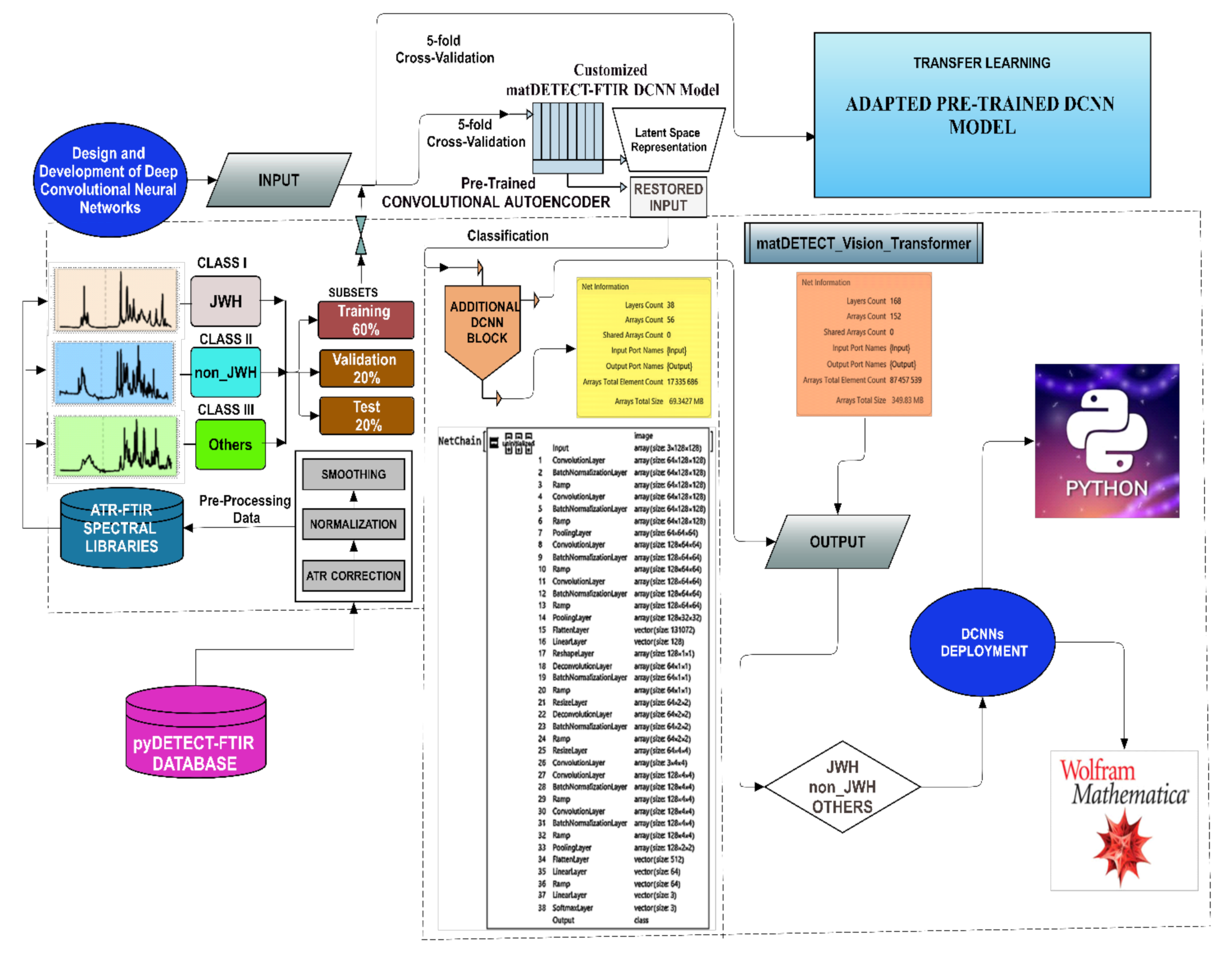
2.6.1. The matDETECT_FTIR DCNN Model

An autoencoder is a type of Artificial Neural Network (ANN) used for learning efficiently data coding in an unsupervised manner. The primary aim of an autoencoder is to learn a representation (encoding) for a dataset, typically for the purpose of dimensionality reduction or feature extraction [30].

The main architecture presented in this article is built upon a custom-designed Convolutional Autoencoder (CAE), which was pre-trained without labels on an extensive Non-Forensic ATR-FTIR Spectral Library comprising approximately 11,000 spectral images. Subsequently, we honed its performance on the second Forensic ATR-FTIR Spectral Library (comprising approximately 10,400 spectral images).

At this stage, we froze the weights of certain layers (typically, the lower layers that learn lower-level features) and trained only the upper layers of the networks. In this step, the DCNN models were trained with the specific labels of the three classes of interest.

This system uses a DCNN that comprises both encoding (encoder) and decoding (decoder) components, along with an additional classification segment. The CAE framework was trained to learn compact representations of the input data (the ATR-FTIR spectral images), which are then used as inputs to the DCNN architecture. Thus, the autoencoder part performs a data pre-processing and feature extraction function before the data are fed into the DCNN model for classification. The training process for this model can be divided into two stages of learning, i.e., unsupervised learning and supervised learning.

Unsupervised learning involves the process where the encoder and decoder of the CAE architecture cooperate to learn latent representations of the input data. During this phase, the model trains to compress data into a reduced latent space—referred to as representation learning—through the encoder and then attempts to reconstruct the input data via the decoder. This segment of the procedure, efficient in deriving a compact representation of the data from the extensive dataset, does not need labels, as the model is trained to replicate the input data.

Supervised learning embodies the process wherein an additional classification component is appended to the autoencoder network. At this juncture, the model employs the latent representations ascertained by the autoencoder to perform a classification task, which is inherently supervised. The model is trained to associate these latent representations with the corresponding class labels [58].

Therefore, the architecture depicted integrates both unsupervised learning (through the Convolutional Autoencoder) and supervised learning (via the added classification component). Our approach exemplifies a hybrid technique, also recognized as semi-supervised learning, which amalgamates the strengths of both learning paradigms. Pre-training via unsupervised learning can augment the performance of the model, especially when labeled data are in paucity [59].

In determining the final architecture, we used the Python and Wolfram Mathematica programming platforms. The design process involved iterative ablation experimentation, which included both the addition and removal of various layers (

Table 4. Ablation experiments for the matDETECT_FTIR DCNN model.

Component or Layer Ablated	Effect on Classification (Macro-F1 Score)	Effect on Detection (Specificity)	Overall Accuracy (%)
Full Network (matDETECT)	0.9037	0.9728	96.16
Without Convolutional Autoencoder	0.8832 (−0.0205)	0.9625 (−0.0103)	93.8 (−2.36)
Omitted 1 to 3 Convolution Layers	0.8652–0.8832 (−0.0385 to −0.0205)	0.9555–0.9605 (−0.0173 to −0.0123)	92.2–93.6 (−3.96 to −2.56)
Omitted 1 to 4 Batch Normalization Layers	0.8800–0.8910 (−0.0237 to −0.0127)	0.9610–0.9645 (−0.0118 to −0.0083)	93.7–94.9 (−2.46 to −1.27)
Omitted 1 to 3 Max Pooling Layers	0.8880–0.8980 (−0.0157 to −0.0057)	0.9630–0.9675 (−0.0098 to −0.0053)	94.5–95.5 (−1.66 to −0.66)
Omitted 1 Flatten Layer	0.8971–0.9021 (−0.0066 to −0.0016)	0.9700–0.9715 (−0.0028 to −0.0013)	95.7–96.0 (−0.46 to −0.16)
Omitted 1 Fully Connected Layer	0.9002–0.9042 (−0.0035 to −0.0005)	0.9718–0.9733 (−0.0010 to −0.0005)	96.0–96.3 (−0.16 to −0.14)

). The types of layers experimented with encompassed input layers (1), convolution layers (7), batch normalization layers (8), activation function layers (9, using the Ramp function, which is commonly known as the Rectified Linear Unit or ReLU in standard scientific terms), pooling layers (3), flatten layers (2), linear layers (3), reshape layers (1), deconvolution layers (2), resize layers (2), Softmax layers (1), and ouput layers (1). The resultant architecture is as follows.

• Convolutional Autoencoder Block
  • Encoder Unit
    • Input Layer.
    • Convolution Layer_1 (1792 parameters);
    • Batch Normalization Layer_1 (256 parameters);
    • ReLU Activation_1 (0 parameters);
    • Convolution Layer_2 (36,928 parameters);
    • Batch Normalization Layer_2 (256 parameters);
    • ReLU Activation_2 (0 parameters);
    • Pooling Layer_1 (0 parameters);
    • Convolution Layer_3 (73,856 parameters);
    • Batch Normalization Layer_3 (512 parameters);
    • ReLU Activation_3 (0 parameters);
    • Convolution Layer_4 (147,584 parameters);
    • Batch Normalization Layer_4 (512 parameters);
    • ReLU Activation_4 (0 parameters);
    • Pooling Layer_2 (0 parameters);
    • Flatten Layer_1 (0 parameters);
    • Linear Layer_1 with 128 nodes (16,777,344 parameters).
  • Decoder Unit
    • Reshape layer to dimensions (0 parameters);
    • Deconvolution Layer_1 (73,792 parameters);
    • Batch Normalization Layer_5 (256 parameters);
    • ReLU Activation_5 (0 parameters);
    • Resize layer with a scaling factor of 2 in both dimensions (0 parameters);
    • Deconvolution Layer_2 (36,928 parameters);
    • Batch Normalization Layer_6 (256 parameters);
    • ReLU Activation_6 (0 parameters);
    • Resize layer with a scaling factor of 2 in both dimensions (0 parameters);
    • Convolution Layer_5 (195 parameters).
• Additional Classification Block
  • Convolution Layer_6 (3584 parameters);
  • Batch Normalization Layer_7 (512 parameters);
  • ReLU Activation_7 (0 parameters);
  • Convolution Layer_7 (147,584 parameters);
  • Batch Normalization Layer_8 (512 parameters);
  • ReLU Activation_8 (0 parameters);
  • Pooling Layer_3 (0 parameters);
  • Flatten Layer_2 (0 parameters);
  • Linear Layer_2 with 64 nodes (32,832 parameters);
  • ReLU Activation_9 (0 parameters);
  • Linear Layer_3 with 3 nodes (195 parameters);
  • Softmax Layer (0 parameters).
  • Output Layer.

The DCNN structure was developed from the ground up, involving adjustments and optimizations to several hyperparameters within the framework. This included fine-tuning elements such as the quantity of convolutional and fully connected layers, the assortment of filters, stride values, pooling locales, dimensions, and the configuration of units within the fully connected layers. The determination of these hyperparameters was undertaken manually through a process of iterative experimentation, given the absence of a definitive mathematical model to ascertain the optimal parameters for a distinct dataset.

The final layers of the architecture of the first proposed DCNN model and a visual inquiry of the node graph structure are depicted in Figure 5 and Figure 6 starting with the encoder part of the Convolutional Autoencoder, passing through the decoder part and continuing with the additional classification part specific to the DCNN:

• Layer count = 38;
• Array count = 56;
• Array total element count= 17,335,686;
• Trainable parameters = 17,334,150;
• Non-trainable parameters = 1536;
• Array total size = 69.3427 MB;
• GFLOP/S = 3.126450246.

2.6.2. The matDETECT Vision Transformer DCNN model

The vision transformer trained on the ImageNet competition data model is a deep learning model introduced in 2021 by the team of researchers at Google Research’s Brain Team (

Table 5. Model information for the vision transformer trained on the ImageNet competition data sourced from the Wolfram Neural Net Repository.

Parameters		Statistics			Top-5 Accuracy	Top-1 Accuracy
Model Size	Pach Size	Number of Layers	Total Number of Weights	File Seize (MB)	ImageNet-1k (%)	ImageNet-1k (%)
Base (ViT-B/16)	16	168	86,567,656	346.354	95.318	81.072
Base (ViT-B/32)	32	168	88,224,232	352.981	92.466	75.912
Large (ViT-L/16)	16	324	304,326,632	1217.44	94.638	79.662
Large (ViT-L/32)	32	324	306,535,400	1226.28	93.070	76.972

). Unlike traditional CNNs, which use convolutional layers to process image data, this model applies the transformer architecture, originally designed for natural language processing tasks, to image classification. This model consists of a family of individual nets, and each is identified by a specific parameter combination (Table 5).

In alignment with the objectives and goals of our scientific endeavor, for model design and deployment, we evaluated models from the Wolfram Neural Net Repository, and subsequently, we elected to employ the vision transformer trained on the ImageNet competition data (ViT-B/32) model. The rationale behind selecting this specific model was based on multiple scientific considerations:

• A balance between model size and performance: while the ViT-B/32 offers slightly lower accuracy rates compared to its ViT-B/16 counterpart, it presents a reduced computational burden, making it more feasible for real-time or on-device applications;
• Optimal resource allocation: the ViT-B/32 model offers a good balance between the number of parameters and the Top-1 and Top-5 accuracy scores on ImageNet-1k. This ensures efficient utilization of resources without significantly compromising performance;
• Dataset characteristics: depending on the nature and diversity of our dataset, the ViT-B/32 might have offered certain advantages in feature extraction and representation over other configurations.

  a.

  Self-attention, attention matrix, positional embedding, attention matrix, and distance mechanisms.

We employed a 7 × 7 grid with each patch (token) covering a 32 × 32 spatial region (Figure 7). The key to the transformer architecture of the vision transformer trained on the ImageNet competition data model is the attention mechanism, more specifically, the self-attention mechanism. In the context of transformer models, attention is a measure of the importance of different parts of the input data when making a prediction.

For each pair of input positions (i, j), an attention score is calculated, typically as the dot product of the representations corresponding to the two positions:

Score(i, j) = dot_product (representation (i), representation(j)).

(19)

These scores are then passed through a Softmax function to convert them into probabilities, ensuring the sum of all attention scores for a specific position equals 1. Ultimately, these scores are used to weigh the representations of different positions before they are combined to form the final representation for prediction. This mechanism allows the model to focus on the most relevant parts of the input data for each specific task.

One significant feature of the ViT-B/32 model structure is the attention matrix, which contains the attention scores that reflect how much attention each part of the image is given when processing other parts of the image. For instance, in a 12-head transformer model, an attention matrix would be a 3-dimensional matrix with dimensions {12, 49, 49}, where the first dimension represents the number of attention heads and the second and third dimensions represent the input positions.

The cosine distance between embedded positions is also a significant concept in the model framework. The position embeddings are vectors that represent the position of the input data in a high-dimensional space. The cosine distance is a measure of the similarity between two vectors and is defined as the cosine of the angle between them. This distance can give an idea of how the model perceives the relationships between different positions in the input data.

Visualizing the attention matrix and cosine distances provides valuable insights into the model’s behavior. By transforming the attention matrix into an image, where the color intensity of a pixel corresponds to the attention score of the corresponding position, we may directly observe which areas of the image the model considers important. Visualizing the cosine distances in the embedded positions allows a better understanding of how the model perceives the relationships in different parts of the image [60].

Training, Optimization, and Fine-Tuning

Using the foundation of the ViT-B/32 model for the classification of synthetic cannabinoids has both advantages and disadvantages. On the one hand, the vision transformer systems demonstrated superior performance on several image classification benchmarks, including ImageNet. They can efficiently process images in their entirety, capturing global contextual information that traditional CNNs might miss due to their localized receptive fields. Moreover, using a pre-trained vision transformer model, one can leverage a large amount of pre-existing knowledge, reducing the amount of training data needed and potentially speeding up the learning process.

On the other hand, the transformer architecture tends to be more computationally intensive and memory-demanding compared to CNNs due to its self-attention mechanism. This could be a significant drawback when dealing with large datasets or high-resolution images. Furthermore, the attention mechanism in the vision transformer model could potentially be sensitive to adversarial attacks, where small, intentional changes to the input can lead to incorrect predictions.

Therefore, the decision to use such a model must carefully consider the specific requirements and constraints of the task. In adapting the pre-trained ViT-B/32 model to identify the class signatures of synthetic cannabinoids, we adhered closely to the original model and undertook the following procedures:

• Model Preparation: The pre-trained model was loaded, and the last linear (fully connected or dense) layer was excised to pave the way for the subsequent integration of new layers.
• Network Assembly: A new linear layer and a Softmax layer were added to the altered ViT-B/32 model to mitigate overfitting, calibrate output values facilitating their interpretation as probabilities, and predict the three specified classes (Figure 8).
• Network Training: A 5-fold cross-validation approach was used, which involved partitioning the data into training, validation, and testing sets, thereby facilitating a robust evaluation of the model throughout the training phase (

  Table 6. Training and optimization parameters for the matDTECT Vision Transformer DCNN model.

  Classifier Measurements *	New matDETECT Vision Transformer
  Batches Per Round (Epoch)	8
  Batch Size	32
  Batches Per Second	6.59536
  Mean Batches Per Second	5.8947
  Total Batches	400
  Examples Processed	12800
  Initial Learning Rate	0.001
  Final Learning Rate	0.000574294
  Mean Examples Per Second	188.63
  Total Rounds (Epochs)	50
  Total Training Time (s)	67.8575

  * Note on training configuration: rounds → 50, “ADAM”, “Beta 1” → 0.9, “Beta 2” → 0.999, “Epsilon” → 1/100,000, “Gradient Clipping” → 5, “L2 Regularization” → 0.01, “Learning Rate” → 0.001, “Learning Rate Schedule” → (“Step”, 10, 0.5), “Weight Clipping” → 10.

  ).
• Model Evaluation: A rigorous assessment was performed to gauge the performance of the model, ensuring its reliability and precision in discerning the classes of synthetic cannabinoids.
• Model Preservation: The trained network was secured for future utilization and deployment by exporting it as a “.mx” file.

A comparative analysis of the matDETECT Vision Transformer DCNN, which emerged from the modification and adaptation of the ViT-B/32 model, is presented in

Table 7. A comparative analysis of the matDETECT Vision Transformer DCNN and base (ViT-B/32) model parameters.

Parameters		Statistics
Model Size	Pach Size	Number of Layers	Total Number of Weights	File Seize (MB)	Gflop/s
New matDETECT Vision Transformer	32	168	87,457,539	345.83 MB	8.23
Base (ViT-B/32)	32	168	88,224,232	352.981	8.56

.

3. Results

To ensure a quantitative evaluation of the constructed artificial intelligence architectures, we used advanced analytical tools embedded within the Wolfram Mathematica v. 13.2 software suite. One of the primary utilities harnessed was the classifier measurements tool, which proved very useful throughout the training, validation, and testing stages (Figure 9).

This tool not only simplifies the process of computing critical classification metrics but also offers a comprehensive visualization of the same, enabling an in-depth understanding of model performance. Concurrently, the net train results object tool was indispensable in providing granular insights into the nuances of the training dynamics. It meticulously logged data on loss and performance metrics at each iteration, along with pertinent information on training velocity and associated parameters, thereby offering a holistic view of the model’s evolution during the training phase.

These tools generated a comprehensive suite of measurements or metrics, referred to as properties, which yielded a robust platform for evaluating and contrasting the various features of the models. The metrics encompassed a wide array of elements including, but not limited to, confusion matrix, accuracy, precision and 1-precision, loss, specificity, sensitivity (recall) and 1-recall, macro-F1 score, error rate, and kappa coefficient (

Table 8. Evaluative analysis of the DCNN models based on accuracy, precision, and complementary precision metrics.

Forensic ATR-FTIR Spectral Library (10,425 Images) Macro-Averaged Metrics (Test Set)
DCNN	Accuracy	Precision	1-Precision
matDETECT_FTIR	0.9616	0.8658	0.1341
matDETECT Vision Transformer	0.9738	0.8485	0.1514

,

Table 9. Quantitative assessment of the DCNN models based on specificity, sensitivity (recall), and complementary recall metrics.

Forensic ATR-FTIR Spectral Library (10,425 Images) Macro-Averaged Metrics (Test Set)
DCNN	Specificity	Sensitivity (Recall)	1-Recall
matDETECT_FTIR	0.9728	0.9616	0.0383
matDETECT Vision Transformer	0.9954	0.9758	0.0241

,

Table 10. Analytical evaluation of the DCNN models based on the error rate, class mean cross-entropy, and kappa coefficient insights.

Forensic ATR-FTIR Spectral Library (10,425 Images) Macro-Averaged Metrics (Test Set)
DCNN	Error Rate	Kappa Coefficient
matDETECT_FTIR	0.2391	0.7930
matDETECT Vision Transformer	0.2308	0.8350

and

Table 11. Optimal experimental outcomes from the DCNN models: macro-F1 score and loss analysis.

Forensic ATR-FTIR Spectral Library (10,425 Images) Macro-Averaged Metrics (Test Set)
DCNN	Macro-F1 Score	Loss
matDETECT_FTIR	0.9037	0.1342
matDETECT Vision Transformer	0.9025	0.0979

and Figure 10, Figure 11 and Figure 12), thereby providing a profound insight into the nuances of the performances of the models.

4. Discussion

Upon a rigorous analysis of the presented confusion matrices, coupled with the empirically derived data, several salient aspects emerge regarding the proficiency of the two DCNN models in distinguishing and classifying synthetic cannabinoids, as well as other predominant designer drugs:

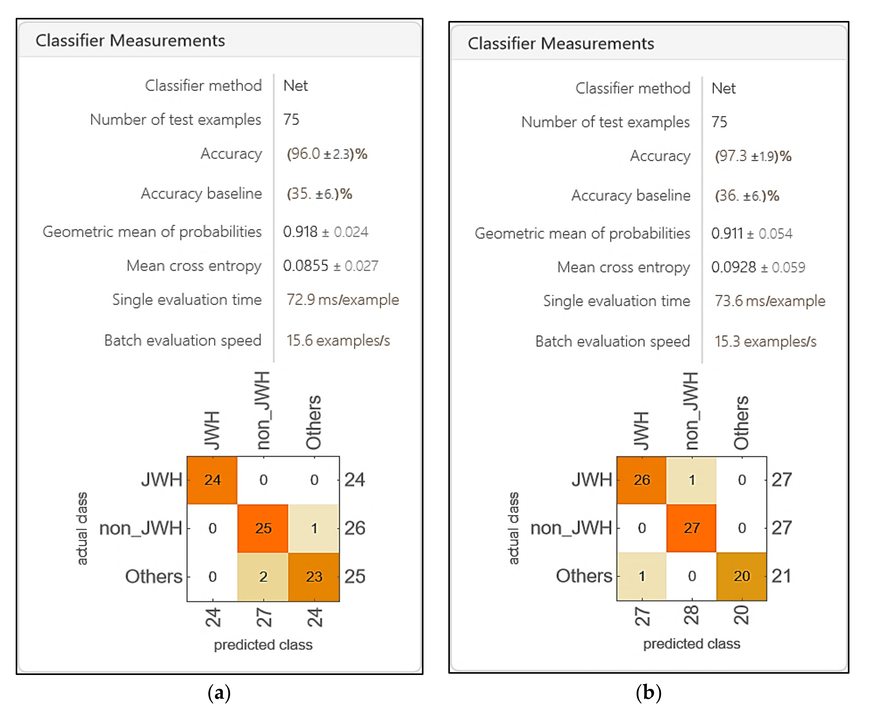
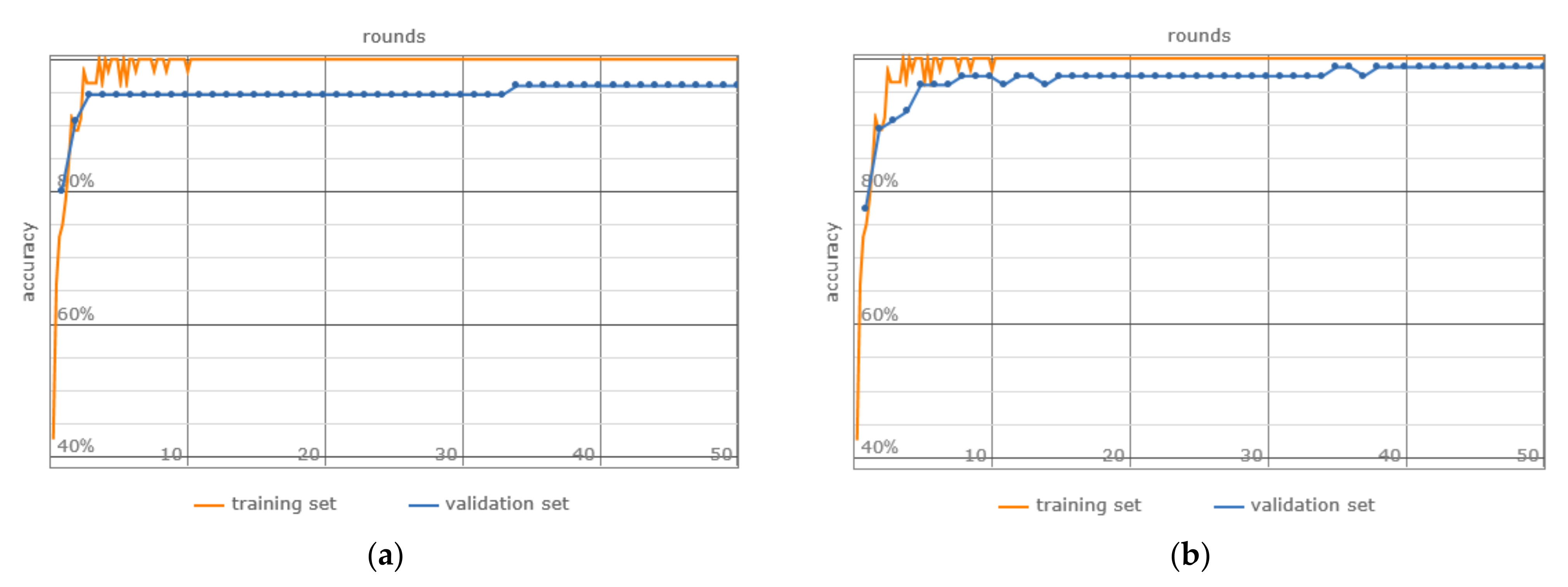
• Accuracy: The matDETECT Vision Transformer model exhibits marginally superior accuracy compared to the matDETECT_FTIR model.
• Precision: Notably, the matDETECT_FTIR model demonstrates elevated precision, suggesting a diminished incidence of false positives.
• Specificity: The matDETECT Vision Transformer model boasts enhanced specificity, implying a more effective detection of true negatives.
• Sensitivity (Recall): Furthermore, the matDETECT Vision Transformer showcases superior sensitivity, indicating a heightened capacity to detect true positives.
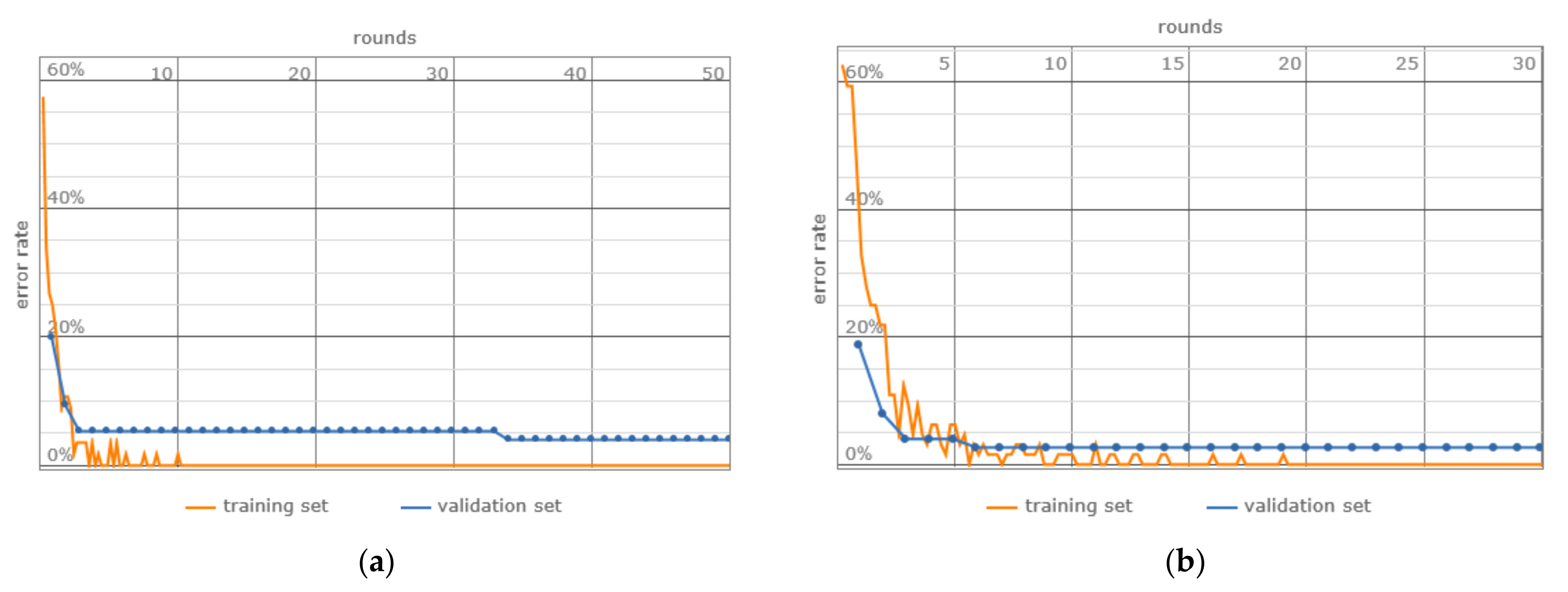
• Error Rate: Although both models present analogous error rates, the matDETECT Vision Transformer registers a marginally reduced rate.
• Kappa Coefficient: Additionally, the matDETECT Vision Transformer evidences an elevated kappa coefficient, signifying an enhanced model concordance.
• Macro-F1 Score: Both models possess comparable macro-F1 scores, insinuating a harmonized equilibrium between precision and recall.
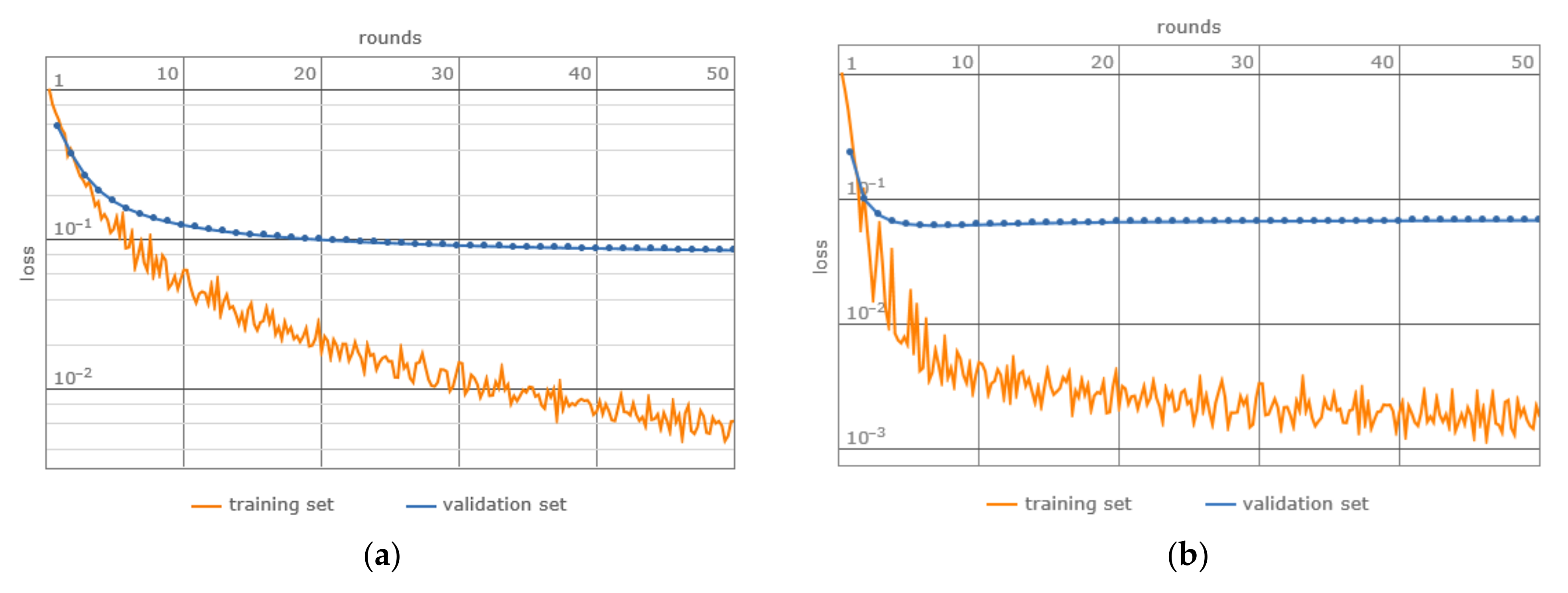
• Loss: The matDETECT Vision Transformer model records a lesser loss, hinting at a potentially superior data fit.

Collectively, the aforementioned models exhibit commendable competence across most assessed metrics, surpassing several contemporary DCNNs documented in prior research, thereby positioning themselves as formidable contenders and arguably more trustworthy alternatives for the discernment and classification of synthetic cannabinoids and other analogous synthetic narcotics. The matDETECT Vision Transformer, with its pronounced specificity and sensitivity, alongside a curtailed error rate, emphasizes its robust performance capabilities.

However, it is worth noting that the observed performance differentials remain relatively subtle. The matDETECT_FTIR model, with its slightly augmented precision, signifies a lesser rate of false positives—a metric that could carry substantial implications contingent on specific forensic requirements. Hence, should the mitigation of false positives be a primary objective, the selection of the matDETECT_FTIR model, considering its enhanced precision, might be a prudent decision.

5. Conclusions

This study presents a significant stride in forensic identification and classification through the development of DCNN systems, showcasing their efficacy in recognizing synthetic cannabinoids and other substances of forensic importance. These intricate architectures, backed by diverse foundations, emphasize the feasibility of employing various pre-trained structures, including custom-designed and open-source frameworks, to tackle inherent complexities in this scientific area. The incorporation of innovative transfer learning strategies, combining supervised and unsupervised paradigms, demonstrates potential in addressing challenges tied to limited datasets. Additionally, the use of Convolutional Autoencoders and ATR-FTIR spectroscopy enhances the accuracy of identification. These systems herald a promising future, offering precision and efficiency, while strategic strategies like data augmentation hold the potential to enhance model performance. Collaborations with emerging technologies could lead to refined and adaptable systems, and addressing false positives becomes paramount. We believe that the results presented in this paper are an important contribution toward an efficient and reliable substance detection of drugs of abuse, contributing to the advancement of computer-aided forensics by offering a scalable solution for psychoactive substance identification and helping law enforcement in tackling the illicit drug trade.

References

1. Alkhuder, K. Attenuated total reflection-Fourier transform infrared spectroscopy: A universal analytical technique with promising applications in forensic analyses. Int. J. Leg. Med. 2022, 136, 1718–1729. [Google Scholar] [CrossRef] [PubMed]
2. Blanco-González, A.; Cabezón, A.; Seco-González, A.; Conde-Torres, D.; Antelo-Riveiro, P.; Piñeiro, Á.; Garcia-Fandino, R. The Role of AI in Drug Discovery: Challenges, Opportunities, and Strategies. Pharmaceuticals 2023, 16, 891. [Google Scholar] [CrossRef]
3. Gupta, R.; Srivastava, D.; Sahu, M.; Tiwari, S.; Ambasta, R.K.; Kumar, P. Artificial intelligence to deep learning: Machine intelligence approach for drug discovery. Mol. Divers. 2021, 25, 1315–1360. [Google Scholar] [CrossRef] [PubMed]
4. Rumelhart, D.E.; Hinton, G.E.; Williams, R.J. Parallel Distributed Processing: Explorations in the Microstructure of Cognition; Learning Internal Representations by Error Propagation; MIT Press: Cambridge, MA, USA, 1986; Volume 1, pp. 318–362. [Google Scholar]
5. Pu, Y.; Gan, Z.; Henao, R.; Yuan, X.; Li, C.; Stevens, A.; Carin, L. Variational autoencoder for deep learning of images, labels and captions. Adv. Neural Inf. Process. Syst. 2016, 29, 2352–2360. [Google Scholar]
6. Ilesanmi, A.E.; Ilesanmi, T.O. Methods for image denoising using convolutional neural network: A review. Complex Intell. Syst. 2021, 7, 2179–2198. [Google Scholar] [CrossRef]
7. Arai, H.; Chayama, Y.; Iyatomi, H.; Oishi, K. Significant dimension reduction of 3D brain MRI using 3D convolutional autoencoders. In Proceedings of the 40th Annual International Conference of the IEEE Engineering in Medicine and Biology Society (EMBC), Honolulu, HI, USA, 17–21 July 2018; pp. 5162–5165. [Google Scholar]
8. Guo, X.; Liu, X.; Zhu, E.; Yin, J. Deep clustering with convolutional autoencoders. In Proceedings of the International Conference on Neural Information Processing 2017, Guangzhou, China, 14–18 November 2017; pp. 373–382. [Google Scholar]
9. Kucharski, D.; Kleczek, P.; Jaworek-Korjakowska, J.; Dyduch, G.; Gorgon, M. Semi-supervised nests of melanocytes segmentation method using convolutional autoencoders. Sensors 2020, 20, 1546. [Google Scholar] [CrossRef]
10. Vaswani, A.; Shazeer, N.; Parmar, N.; Uszkoreit, J.; Jones, L.; Gomez, A.N.; Kaiser, L.; Polosukhin, I. Attention is All you Need. arXiv 2017, arXiv:1706.03762. [Google Scholar]
11. Luong, T.; Pham, H.; Manning, C.D. Effective Approaches to Attention-based Neural Machine Translation. In Proceedings of the Conference on Empirical Methods in Natural Language Processing (ACL) 2015, Lisbon, Portugal, 17–21 September 2015; pp. 1412–1421. [Google Scholar]
12. Islam, S.; Elmekki, H.; Elsebai, A.; Bentahar, J.; Drawel, N.; Rjoub, G.; Pedrycz, W. A Comprehensive Survey on Applications of Transformers for Deep Learning Tasks. arXiv 2023, arXiv:2306.07303 2023. [Google Scholar]
13. Maray, N.; Ngu, A.H.; Ni, J.; Debnath, M.; Wang, L. Transfer Learning on Small Datasets for Improved Fall Detection. Sensors 2023, 23, 1105. [Google Scholar] [CrossRef]
14. Burlacu, C.M.; Gosav, S.; Burlacu, B.A.; Praisler, M. Convolutional Neural Network Detecting Synthetic Cannabinoids. In Proceedings of the International Conference on e-Health and Bioengineering (EHB), Iasi, Romania, 18–19 November 2021. [Google Scholar]
15. Google Research. Vision_Transformer. Available online: https://github.com/google-research/vision_transformer (accessed on 16 March 2023).
16. Wolfram Neural Net Repository. Available online: https://resources.wolframcloud.com/NeuralNetRepository/resources/Vision-Transformer-Trained-on-ImageNet-Competition-Data/ (accessed on 2 June 2023).
17. Dosovitskiy, A.; Beyer, L.; Kolesnikov, A.; Weissenborn, D.; Zhai, X.; Unterthiner, T.; Dehghani, M.; Minderer, M.; Heigold, G.; Gelly, S.; et al. An Image Is Worth 16 × 16 Words: Transformers for Image Recognition at Scale. arXiv 2021, arXiv:2010.11929v2. [Google Scholar]
18. Wolfram Research, I. Mathematica Version 13.3; Wolfram Research, Inc.: Champaign, IL, USA, 2023. [Google Scholar]
19. Hellmann, D. The Python 3 Standard Library by Example, 2nd ed.; Addison-Wesley Professional: Boston, NA, USA, 2017. [Google Scholar]
20. Pereira, L.S.; Lisboa, F.L.; Neto, J.C.; Valladão, F.; Sena, M.M. Direct classification of new psychoactive substances in seized blotter papers by ATR-FTIR and multivariate discriminant analysis. Microchem. J. 2017, 133, 96–103. [Google Scholar] [CrossRef]
21. Pereira, L.S.; Lisboa, F.L.; Neto, J.C.; Valladão, F.N.; Sena, M.M. Screening method for rapid classification of psychoactive substances in illicit tablets using mid infrared spectroscopy and PLS-DA. Forensic Sci. Int. 2018, 288, 227–235. [Google Scholar] [CrossRef] [PubMed]
22. Du, Y.; Hua, Z.; Liu, C.; Lv, R.; Jia, W.; Su, M. ATR-FTIR combined with machine learning for the fast non-targeted screening of new psychoactive substances. Forensic Sci. Int. 2023, 349, 111761. [Google Scholar] [CrossRef] [PubMed]
23. Tsujikawa, K.; Yamamuro, T.; Kuwayama, K.; Kanamori, T.; Iwata, Y.T.; Miyamoto, K.; Kasuya, F.; Inoue, H. Application of a portable near infrared spectrometer for presumptive identification of psychoactive drugs. Forensic Sci. Int. 2014, 242, 162–171. [Google Scholar] [CrossRef]
24. Radhakrishnan, A.; Damodaran, K.; Soylemezoglu, A.C.; Uhler, C.; Shivashankar, G.V. Machine Learning for Nuclear Mechano-Morphometric Biomarkers in Cancer Diagnosis. Sci. Rep. 2017, 7, 17946. [Google Scholar] [CrossRef]
25. Koutsoukas, A.; Monaghan, K.; Li, X.; Huan, J. Deep-learning: Investigating deep neural networks hyper-parameters and comparison of performance to shallow methods for modeling bioactivity data. J. Cheminform. 2017, 9, 42. [Google Scholar] [CrossRef]
26. Mendenhall, J.; Meiler, J. Improving quantitative structure-activity relationship models using Artificial Neural Networks trained with dropout. J. Comput.-Aided Mol. Des. 2016, 30, 177–189. [Google Scholar]
27. Wallach, I.; Dzamba, M.; Heifets, A. AtomNet: A Deep Convolutional Neural Network for Bioactivity Prediction in Structure-based Drug Discovery. arXiv 2015, arXiv:1510.02855. [Google Scholar]
28. Shi, W.; Singha, M.; Srivastava, G.; Pu, L.; Ramanujam, J.; Brylinski, M. Pocket2Drug: An Encoder-Decoder Deep Neural Network for the Target-Based Drug Design. Front. Pharmacol. 2022, 13, 837715. [Google Scholar] [CrossRef]
29. Sun, C.; Cao, Y.; Wei, J.M.; Liu, J. Autoencoder-based drug-target interaction prediction by preserving the consistency of chemical properties and functions of drugs. J. Bioinform. 2021, 37, 3618–3625. [Google Scholar] [CrossRef]
30. Pintelas, E.; Livieris, I.E.; Pintelas, P.E. A Convolutional Autoencoder Topology for Classification in High-Dimensional Noisy Image Datasets. Sensors 2021, 21, 7731. [Google Scholar] [CrossRef] [PubMed]
31. Simonyan, K.; Zisserman, A. Very Deep Convolutional Networks for Large-Scale Image Recognition. arXiv 2014, arXiv:1409.1556. [Google Scholar]
32. Huang, G.; Liu, Z.; Van Der Maaten, L.; Weinberger, K.Q. Densely connected convolutional networks. In Proceedings of the IEEE Conference on Computer Vision and Pattern Recognition, Honolulu, HI, USA, 21–26 July 2017; pp. 4700–4708. [Google Scholar]
33. Sandler, M.; Howard, A.; Zhu, M.; Zhmoginov, A.; Chen, L.C. Mobilenetv2: Inverted residuals and linear bottlenecks. In Proceedings of the IEEE Conference on Computer Vision and Pattern Recognition, Salt Lake City, UT, USA, 18–22 June 2018; pp. 4510–4520. [Google Scholar]
34. He, K.; Zhang, X.; Ren, S.; Sun, J. Deep residual learning for image recognition. In Proceedings of the IEEE Conference on Computer Vision and Pattern Recognition, Honolulu, HI, USA, 27–30 June 2016; pp. 770–778. [Google Scholar]
35. Szegedy, C.; Vanhoucke, V.; Ioffe, S.; Shlens, J.; Wojna, Z.B. Rethinking the Inception Architecture for Computer Vision. In Proceedings of the IEEE Conference on Computer Vision and Pattern Recognition, Las Vegas, NV, USA, 27–30 June 2016; pp. 2818–2826. [Google Scholar]
36. Devlin, J.; Chang, M.W.; Lee, K.; Toutanova, K. BERT: Pre-training of Deep Bidirectional Transformers for Language Understanding. In Proceedings of the Conference of the North American Chapter of the Association for Computational Linguistics: Human Language Technologies, Minneapolis, MN, USA, 2–7 June 2019; Volume 1 (Long and Short Papers), pp. 4171–4186. [Google Scholar]
37. Chen, H.; Wang, Y.; Guo, T.; Xu, C.; Deng, Y.; Liu, Z.; Ma, S.; Xu, C.; Xu, C.; Gao, W. Pre-trained image processing transformer. arXiv 2021, arXiv:2012.00364. [Google Scholar]
38. Ali, L.; Alnajjar, F.; Jassmi, H.A.; Gocho, M.; Khan, W.; Serhani, M.A. Performance Evaluation of Deep CNN-Based Crack Detection and Localization Techniques for Concrete Structures. Sensors 2021, 21, 1688. [Google Scholar] [CrossRef]
39. Alshammari, H.; Gasmi, K.; Ben Ltaifa, I.; Krichen, M.; Ben Ammar, L.; Mahmood, M.A. Olive Disease Classification Based on Vision Transformer and CNN Models. Comput. Intell. Neurosci. 2022, 2022, 3998193. [Google Scholar] [CrossRef]
40. Liu, W.; Li, C.; Xu, N.; Jiang, T.; Rahaman, M.M.; Sun, H.; Wu, X.; Hu, W.; Chen, H.; Sun, C.; et al. CVM-Cervix: A Hybrid Cervical Pap-Smear Image Classification Framework Using CNN, Visual Transformer and Multilayer Perceptron. arXiv 2022, arXiv:2206.00971. [Google Scholar] [CrossRef]
41. Gheflati, B.; Rivaz, H. Vision Transformers for Classification of Breast Ultrasound Images. In Proceedings of the Conference of the IEEE Engineering in Medicine & Biology Society (EMBC), Glasgow, UK, 11–15 July 2022; pp. 480–483. [Google Scholar]
42. Liu, Y.; Yao, W.; Qin, F.; Zhou, L.; Zheng, Y. Spectral Classification of Large-Scale Blended (Micro)Plastics Using FT-IR Raw Spectra and Image-Based Machine Learning. Environ. Sci. Technol. 2023, 57, 6656–6663. [Google Scholar] [CrossRef]
43. Zhou, W.; Qian, Z.; Ni, X.; Tang, Y.; Guo, H.; Zhuang, S. Dense Convolutional Neural Network for Identification of Raman Spectra. Sensors 2023, 23, 7433. [Google Scholar] [CrossRef]
44. Intel. Available online: https://www.intel.com/content/www/us/en/docs/onemkl/developer-guide-windows/2023-0/overview-intel-distribution-for-linpack-benchmark.html (accessed on 26 September 2023).
45. Dongarra, J.; Bunch, J.; Moler, C.; Stewart, G.W. LINPACK Users Guide; SIAM: Philadelphia, PA, USA, 1979. [Google Scholar]
46. Dongarra, J. Performance of Various Computers Using Standard Linear Equations Software; Computer Science Technical Report Number CS-89-85, TN 37996-1301; University of Tennessee: Knoxville, TN, USA, 2014; Available online: http://www.netlib.org/benchmark/performance.ps (accessed on 25 September 2023).
47. TOP500. Available online: https://www.top500.org/statistics/list/ (accessed on 27 September 2023).
48. Burlacu, C.M.; Burlacu, A.C.; Praisler, M. Physico-chemical analysis, systematic benchmarking, and toxicological aspects of the JWH aminoalkylindole class-derived synthetic JWH cannabinoids. Ann. Univ. Dunarea Jos Galati Fascicle II Math. Phys. Theor. Mech. 2021, 44, 34–45. [Google Scholar] [CrossRef]
49. Elreedy, D.; Atiya, A. A Comprehensive Analysis of Synthetic Minority Oversampling Technique (SMOTE) for Handling Class Imbalance. Inf. Sci. 2019, 505, 32–64. [Google Scholar] [CrossRef]
50. Menges, F. Spectragryph—Optical Spectroscopy Software, Version 1.2.16.1. 2022. Available online: http://www.effemm2.de/spectragryph/ (accessed on 5 September 2023).
51. Wenig, P.; Odermatt, J. OpenChrom: A cross-platform open-source software for the mass spectrometric analysis of chromatographic data. BMC Bioinform. 2010, 11, 405. [Google Scholar] [CrossRef] [PubMed]
52. Alomar, K.; Aysel, H.I.; Cai, X. Data Augmentation in Classification and Segmentation: A Survey and New Strategies. J. Imaging 2023, 9, 46. [Google Scholar] [CrossRef] [PubMed]
53. Goodfellow, I.; Pouget-Abadie, J.; Mirza, M.; Xu, B.; Warde-Farley, D.; Ozair, S.; Courville, A.; Bengio, Y. Generative Adversarial Networks. Adv. Neural Inf. Process. Syst. 2020, 63, 139–144. [Google Scholar] [CrossRef]
54. Radford, A.; Metz, L.; Chintala, S. Unsupervised Representation Learning with Deep Convolutional Generative Adversarial Networks. arXiv 2015, arXiv:1511.06434. [Google Scholar]
55. Lee, M. Recent Advances in Generative Adversarial Networks for Gene Expression Data: A Comprehensive Review. Mathematics 2023, 11, 3055. [Google Scholar] [CrossRef]
56. Lin, T.Y.; Goyal, P.; Girshick, R.; He, K.; Dollár, P. Focal Loss for Dense Object Detection. In Proceedings of the IEEE International Conference on Computer Vision (ICCV), Venice, Italy, 22–29 October 2017; pp. 2999–3007. [Google Scholar] [CrossRef]
57. Kingma, D.; Ba, J. Adam: A Method for Stochastic Optimization. In Proceedings of the International Conference on Learning Representations, ICLR 2015, San Diego, CA, USA, 7–9 May 2015. [Google Scholar]
58. An, Q.; Rahman, S.; Zhou, J.; Kang, J.J. A Comprehensive Review on Machine Learning in Healthcare Industry: Classification, Restrictions, Opportunities and Challenges. Sensors 2023, 23, 4178. [Google Scholar] [CrossRef]
59. van Engelen, J.E.; Hoos, H.H. A survey on semi-supervised learning. Mach. Learn. 2020, 109, 373–440. [Google Scholar] [CrossRef]
60. Machine Learning Mastery. Available online: https://machinelearningmastery.com/the-transformer-attention-mechanism/ (accessed on 6 September 2023).
Figure 1. Overview of the development process for the matDETECT DCNN model detecting synthetic cannabinoids.
Inventions 08 00129 g001
Figure 2. Comprehensive visualization of the ATR-FTIR spectral image libraries used for the development of synthetic cannabinoid detection systems.
Inventions 08 00129 g002
Figure 3. Refined spectral image preprocessing techniques: ATR correction, normalization, and smoothing.
Inventions 08 00129 g003
Figure 4. Data augmentation strategies: affine transformed, flipped top–bottom, flipped left–right, rotated (45°), rotated (90°), rotated (180°), sheared, noisy, inverted, horizontal derivative, cropped, perspective transformed, magnified.
Inventions 08 00129 g004
Figure 5. The operational framework of the matDETECTION_FTIR DCNN model.
Inventions 08 00129 g005
Figure 6. Node-based architectural framework of the matDETECT_FTIR DCNN system.
Inventions 08 00129 g006
Figure 7. Illustration of the discretized image representation using a 7 × 7 grid, where each patch (token) spans a 32 × 32 spatial region: red highlights object areas of interest, while yellow denotes less relevant regions. The figure also showcases positional embedding, and the attention matrix of dimensions 49 × 768: varying blue shades reflect attention levels, with darker tones suggesting diminished focus and red to pink tones emphasizing areas of higher attention. Additionally, the matrix of distances from the top-left patch across different heads uses blue for shorter distances, transitioning through yellow and brown to red for increasing distances from the top-left patch, all within the matDETECT Vision Transformer DCNN.
Inventions 08 00129 g007
Figure 8. Detailed structural representation of the attention mechanism on the matDTECT Vision Transformer DCNN.
Inventions 08 00129 g008
Figure 9. The preliminary evaluation report of the classifier measurements tool (classifier method, number of test examples, accuracy, accuracy baseline, geometric mean of probabilities, mean cross entropy, single evaluation time, batch evaluation speed and confusion matrix): (a) On the matDETECT_FTIR DCNN model; (b) On the matDETECT Vision Transformer DCNN model.
Inventions 08 00129 g009
Figure 10. The accuracy metric on the test set: (a) the matDETECT_FTIR DCNN model; (b) the matDETECT Vision Transformer DCNN model.
Inventions 08 00129 g010
Figure 11. The loss metric on the test set: (a) the matDETECT_FTIR DCNN model; (b) the matDETECT Vision Transformer DCNN model.
Inventions 08 00129 g011
Figure 12. The error rate metric on the test set: (a) the matDETECT_FTIR DCNN model; (b) the matDETECT Vision Transformer DCNN model.
Inventions 08 00129 g012