From Sparse to Dense Representations in Open Channel Flow Images with Convolutional Neural Networks

Abstract

Convolutional neural networks (CNN) have been widely adopted in fluid dynamics investigations over the past few years due to their ability to extract and process fluid flow field characteristics. Both in sparse-grid simulations and sensor-based experimental data, the establishment of a dense flow field that embeds all spatial and temporal flow information is an open question, especially in the case of turbulent flows. In this paper, a deep learning (DL) method based on computational CNN layers is presented, focusing on reconstructing turbulent open channel flow fields of various resolutions. Starting from couples of images with low/high resolution, we train our DL model to efficiently reconstruct the velocity field of consecutive low-resolution data, which comes from a sparse-grid Direct Numerical Simulation (DNS), and focus on obtaining the accuracy of a respective dense-grid DNS. The reconstruction is assessed on the peak signal-to-noise ratio (PSNR), which is found to be high even in cases where the ground truth input is scaled down to 25 times.

1. Introduction

The term open channel flow describes a free surface flow where a liquid–air contact surface exists and atmospheric pressure is applied. Therefore, free-surface flows include all flows in natural and man-made ducts, and most of the time, these are turbulent flows. The exceptions are few and concern very low-depth flows [1,2]. Turbulence causes the occurrence of vortices within a wide range of length and time scales that interact in a dynamically complex way. In general, in engineering applications, the investigation focuses either on experiments or numerical simulations (or both). Additional problems may arise, though, and experiments may end up with limited or noisy measurements, while numerical simulations for complex and large systems oftentimes demand high computational times and computer power [3].

Experiments on open channel flows have reported inherent difficulties in measurements very close to the free surface, where fluctuations of the root-mean-square (rms) velocity in the vertical direction are observed [4,5,6,7]. Moreover, it was found that the fluctuations in the vertical direction were damped in contrast to those in the tangential direction, which were amplified close to the free surface. It is therefore not surprising that a significant part of the scientific community has devoted itself to the development of numerical models to study the effects of turbulence, since its inclusion in engineering applications is significant. The methods, depending on the level of precision they offer, are classified in the following categories: (a) RANS (Reynolds Averaged Navier–Stokes), (b) LES (Large Eddy Simulations), and (c) DNS (Direct Numerical Simulations) [8,9,10].

More specifically, in the turbulence models for RANS equations, the objective is focused on the mean flow and the way the turbulence affects its properties. Before applying any numerical method, the Navier–Stokes (N-S) equations are written in the form of time-averages. In the RANS flow equations, additional terms appear due to the interactions between the turbulent fluctuations, so these terms have to be modeled in turn with turbulence models. It is worth noticing that the computational resources required for reasonably accurate results related to the flow field are relatively simple, which is why RANS ranks at the bottom of the hierarchy in terms of computational power requirements for common engineering problems [11]. The principal concept of the LES method is based on the detection of the behavior and development of Large Eddies. The method involves spatial filtering of the unsteady N-S before the calculations, which aims to keep the largest scales and discard the smallest ones. The equations of non-steady flow have to be solved, where the computational cost requirements in terms of storage and volume of calculations are higher compared to the RANS method, and, for this reason, LES is an intermediate computation form for turbulent flows [12,13].

On the other hand, DNS has been the method of choice when accuracy is the question and has contributed remarkably to turbulence research in the last decades [14]. The continuity and the N-S equations for incompressible constant viscosity turbulent flow constitute a closed system of four equations with the following four unknown variables: velocity components u, v, and w (in x-, y-, and z-directions, respectively), and pressure, p. This set of equations is taken as the starting point in DNS, and a transition solution is developed in a sufficiently dense spatial mesh (in order to resolve the Kolmogorov length scales in which the energy dissipation takes place) with sufficiently short time steps to capture even the smallest eddies and the “fastest” fluctuations. The advantages of DNS include the fact that no empirical turbulence model is required, whereas one of the main disadvantages of the method, which makes it not widely used in industry, is that the calculations are very demanding in terms of computational resources [15].

Nevertheless, the increased computational effort inherent in DNS and other numerical formulations, both in terms of time and hardware needs, has opened the way to adopt novel computational techniques stemming from machine learning (ML) [16]. Aerodynamic coefficient prediction, turbulence modeling, transitional flow modeling, and flow reconstruction are just a few fields of application [17,18]. More specifically, deep learning (DL) techniques have attracted a lot of interest, especially for their use as surrogate models in computational fluid dynamics (CFD). DL models can deal with complex mathematical concepts through a layered network of interconnected nodes, and they can be easily applied to applications involving data in 2D and 3D dimensions, where the computational domain is discretized using meshes. In CFD, a dense grid leads to higher accuracy, and this corresponds to a deeper network in the DL method. Therefore, the alternative solution of employing DL methods can improve flow estimation and diminish computational time.

A constantly evolving field of research lately with ever-increasing accuracy, super resolution (SR), utilizes high-resolution (HR) data reconstruction using sparse measurements with DL approaches [19,20]. To achieve this, convolutional neural networks (CNNs), Variational Autoencoders (VAEs), and generative adversarial networks (GANs) [21,22,23,24] are among the most common architectures utilized. A relevant example has utilized a U-Net type architecture with CNN layers achieving satisfying results in flow image reconstruction [25]. Even with lightweight networks, performance is fine, suggesting a fast and practical solution for handling turbulent flow data. Real-time reconstruction has also been achieved within a spatio-temporal high-resolution (HR) flow field from low-resolution (LR) data using CNNs and MST-UNet [26]. In this model, the HR images of the previous frame and the LR images of the current frame pose as the model input in a multi-scale manner. The U-Net architecture has been widely employed in image segmentation tasks [27]. Another successful implementation, ResNet, has been introduced to address the vanishing gradient problem [28]. The NuNet architecture has also achieved remarkable performance when compared with the OpenFoam AMR solver [29], presenting impressive discriminative capabilities.

A comparison of SR model performance is usually made based on the value of the peak signal-to-noise ratio (PSNR). Common values for successful models range between PSNR = 30–40 dB. Nevertheless, higher values have been reported by the multiple path super-resolution convolutional neural network (MPSRC) [30], which has given a value of PSNR > 50.0 dB, while the recent deep learning flow image (DELFI) has also achieved high accuracy and architecture simplicity, with PSNR ≅ 39 dB [31].

In the present paper, open channel flow image data derived from DNS simulations are employed to train a super-resolution model, the Upscaling CNN (UpCNN), making it capable of upscaling sparse/coarse data onto a high-resolution (HR) field. The architecture of UpCNN is based on consecutive CNN layers in an encoding/decoding manner, with residual connections to ensure proper information exchange. The proposed architecture achieves high performance on fluid image reconstruction tasks, with PSNR = 51.5 dB, in short training time, without the need to occupy complex computer architectures and memory, as it can just run on common computer hardware. To achieve efficient network training, HR images are first scaled down to a factor of 5–25 and enter the network along with their respective HR images in pairs, so as to create an upscaling mechanism able to reconstruct coarse fields into their fine analog. The reconstruction results on our open channel flow DNS data are very close to the HR images, suggesting that the method can be employed in relevant fluid mechanics applications as a complimentary method to time- and resource-intensive DNS simulations.

2. Materials and Methods

2.1. Super-Resolution Components

2.1.1. Convolutional Neural Networks

Convolutional neural networks are the core components of an SR architecture. In a CNN architecture, input data (typically 2D image data) goes through convolutional layers, which transform spatial information into a series of filters to identify local patterns. The network uses a combination of pooling layers, convolutions, and non-linear activation functions to learn hierarchical representations. In order to efficiently deal with big data, spatial dimensions can be reduced through pooling, while global patterns are captured by fully connected layers. Training CNNs involves the minimization of a loss function by modifying network weights through backpropagation [32]. Such architectures are excellent at imaging applications, automatically picking up characteristics and patterns.

2.1.2. Generative Models VAEs-GANs

A type of generative model in the fields of machine learning (ML) and AI are Variational Autoencoders (VAEs). VAEs consist of an encoder, which takes input data and maps it to a probabilistic latent space, and a decoder, which generates output data and reconstructs the input data as accurately as possible [33]. VAEs work on the fundamental premise of acquiring a mapping between a straightforward and constant distribution and the probability distribution of the data [34]. On the other hand, GANs are an alternative class of AI algorithms used in unsupervised learning (UL) and consist of two parts. The first part (the generator) generates new data, and the second part (the discriminator) assesses the generated data, classifying it as real or fake data [35]. Great reconstruction results have also been obtained by an innovative sub-filter modeling method utilizing GANs for reactive turbulent flows [36].

2.1.3. Physics-Informed Neural Networks (PINNs)

To connect ML with physics principles by means of partial differential equations (PDEs), the Physics-Informed Neural Networks (PINNS) have emerged. They are a class of ML that incorporates knowledge from physics equations into the ML training process [37]. They include an additional physics-informed loss term in addition to the standard loss function used for training, adhering to physical laws [38]. Therefore, during the training process, the NN learns from both the input/output data and the physics-informed loss term [39]. A new method of scaling up PINNs to solve arbitrary high-dimensional PDEs is presented in [40]. The performance of the PINN/Resnet block has been investigated by employing Burger’s equation with a discontinuous solution and the Navier–Stokes (N-S) equation with a continuous solution [41]. The findings have clearly shown that Res-PINN exhibits greater predictive power when compared to traditional DL methods.

2.1.4. LSTM Networks

In scientific and engineering practice, there are often scenarios where modeling temporal dependencies, handling sequential data, and capturing long-term information need to be confronted at the same time. To this end, Long Short-Term Memory (LSTM) networks are suggested [42]. These networks are a special type of recurrent neural network (RNN), containing memory cells to store information over a long period of time. These cells have an internal structure that allows them to decide whether to forget, keep, or write the information. The flow of information is controlled through gates, which dynamically adjust [43].

2.2. Simulation and Data Augmentation

2.2.1. Open Channel Flow Data

In order to obtain accurate data for training and validation of an SR imaging network, DNS of an open-channel turbulent flow has been conducted. The selection of this geometry has been based on the premise that the open channel serves as a test bed case for many turbulent flow models, due to the interesting flow physics phenomena that arise and its wide application in engineering and environmental space.

The focus of this paper has been on testing an SR algorithm in the turbulent regime, where the bulk Reynolds number is $R{e}_b=\mathrm{11,200}$. For the numerical modeling of the flow, the OpenFoam finite volume algorithm has been used. OpenFoam is an open-source algorithmic suite that has been previously validated in cases of turbulent open-channel Newtonian and non-Newtonian flows [44,45]. The governing equations that have been solved by the finite volume algorithm are the ones that describe the incompressible turbulent flow and are mathematically expressed in the non-dimensional form of Equations (1) and (2).

$$\nabla \cdot \mathbf{u}=0$$

(1)

$$\mathrm{ }\frac{\partial \mathit{u}}{\partial t}+\left(\mathit{u}\mathrm{ }\cdot \mathrm{ }\nabla \right)\mathrm{ }\mathit{u}=-\mathrm{ }\nabla P+\frac{1}{Re}{\nabla }^2\mathrm{ }\mathit{u}$$

(2)

Equations (1) and (2) represent the continuity and momentum equations for incompressible flow. The variables in these equations represent the non-dimensional velocity vector (u) and the non-dimensional pressure (P). Time is denoted by t, while Re stands for the non-dimensional Reynolds number. In order to arrive at the non-dimensional form of Equations (1) and (2), characteristic variables have been chosen. The characteristic length of the channel has been represented by δ, while its total height is set as h = 2δ. Finally, for the characteristic velocity, the symbol $U_0$ has been used, with the zero-subscript indicating cross-sectional average quantities. Accordingly, the bulk Reynolds number is equal to $R{e}_b=\frac{\rho U_{0}2h}{\mu }$, where ρ and μ represent the fluid density and dynamic viscosity, respectively.

OpenFoam features a large variety of available numerical models that can be utilized for flow modeling. Since the goal of the present research has been to conduct DNS to obtain our dataset, coupling of momentum and pressure through the pressure-implicit split-operator (PISO) method is the choice. The PISO algorithm has already been extensively tested by previous studies and has been proven to require less CPU time [46,47]. At the same time, the algorithm is robust and accurate as well. As far as the numerical schemes are concerned, third-order space-aware and second-order implicit backward-time-aware schemes have been selected.

The flow setup consists of a simple model that incorporates flow between a free surface and a bottom plate with slip and no-slip boundary conditions, respectively. The total height between the free surface and the bottom plate is h = 2δ, while the size in the other two directions has been set to 3πδ and 2πδ (see Figure 1). In the streamwise and spanwise directions, periodic boundary conditions are imposed.

Finally, regarding the spatial grid resolution of the flow field, two different cases have been studied. The first one (case 2), which serves as the high-resolution grid case, has a grid size of 128 × 132 × 128 elements in the streamwise, wall-normal, and spanwise directions, respectively. Resolution, as well as domain size, have been chosen appropriately in order to ensure that the dynamics and flow physics are captured correctly by the present setup. The chosen values have been previously proven to accurately describe dynamics and flow physics, as early as the original work of Kim et al. [48]. More recently, the implied DNS code has been validated against experimental and well-established DNS results with excellent agreement [44,45]. The second case (case 2), which serves as the coarse grid resolution case, has a grid size of 64 × 64 × 64 elements in the same respective directions. In addition to the difference in result accuracy between the two different spatial grid resolution cases, computational times differ naturally as well. A direct comparison between the two cases could yield approximately double the computational time for the finer grid case to obtain the correct results. An increased burden of computational resources for the finer grid case is also directly connected to the above observation.

After the simulations have reached a statistically steady state, data and results have been exported. For the purpose of the present study, two-dimensional (2D) instantaneous velocity fields have been exported along the x-y plane (mid-vertical plane) for 50 consecutive time steps in both HR and LR.

2.2.2. Data Curation

The DNS-extracted high-resolution (HR) dataset consists of 50 RGB (red, green, and blue) images, 40 of which are fed to the training network and the rest are kept for validation purposes (80–20%, respectively). At first, a data augmentation step is considered [20,49], where the HR images are employed to create a richer dataset to effectively train the model (Figure 2). Images are scaled down by a factor of 5, 10, 15, 20, and 25, which results in blurred instances of the HR, from slight blurring (scale = 5) to extra sparse grids and practically tiny images (scale = 25). Details are given in

Table 1. Input data for model training and validation, with number of training images (N_t), number of validation images (N_v), and image dimensions (height × width). The total training set contains 200 images, and the validation set contains 50 images.

	Nt	Nv	(H × W)
HR	40	10	262 × 1176
LR5	40	10	52 × 235
LR10	40	10	26 × 118
LR15	40	10	17 × 78
LR20	40	10	13 × 59
LR25	40	10	10 × 47

.

The creation of such an artificial training dataset is common practice in the field of super-resolution applications [25,50,51]. The procedure that follows takes an HR image and its LR counterpart, feeds the model with this couple, and finds correlations between them so as to be able to make this upscaling from an unseen LR image in the future. For example, when sparse-grid simulation (e.g., from RANS) images are fed, the model will be able to provide their HR counterpart. This is why it is crucial to effectively train the network in the first place.

A more detailed view of the dataset is given in Figure 3. Figure 3a shows the produced images for all scales considered, while Figure 3b shows the flow at some representative timesteps between 1 and 50. Furthermore, a new coarse dataset, which is the result of another DNS simulation that runs for the same input conditions but with a sparser grid (64³ elements), is shown in Figure 3c. The sparser grid contains much less information, but it has the advantage of running in substantially shorter times. Thus, even though the resolution of images in both cases is the same, the ones stemming from the coarser grid dataset offer less information. There is no direct correspondence between these images and an HR set, so we will keep them after the model is trained to reconstruct the HR dataset from scratch.

3. Results

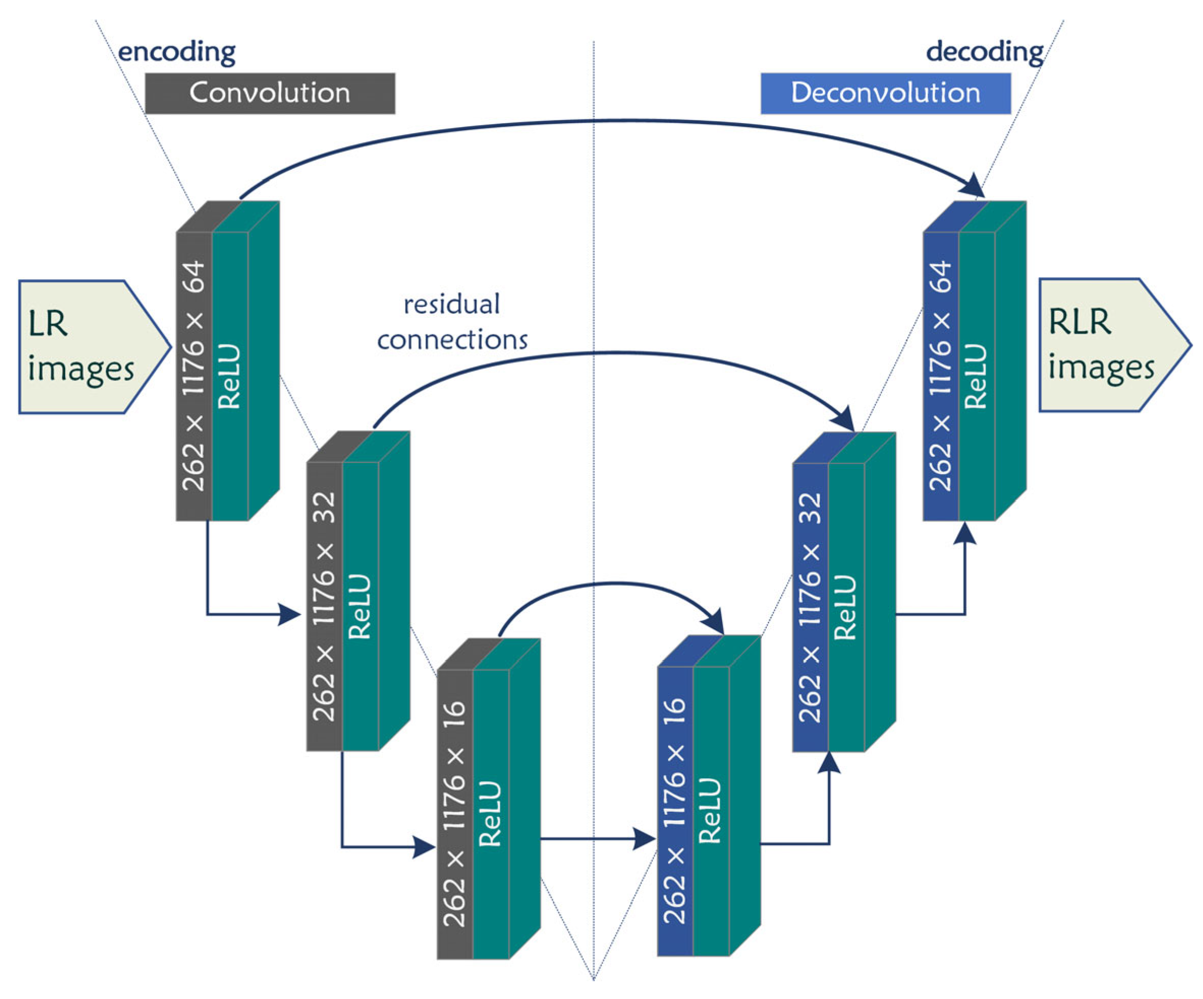
3.1. UpCNN Architecture

To implement the super-resolution method for DNS image data, a U-net type [27] up-scaling model (UpCNN) is proposed (Figure 4). In this architecture, an encoder and a decoder branch are created, with several convolutional layers. In the encoder branch, a convolutional kernel, k, applies to an input image, X, and outputs a series of images (filters), each one featuring image characteristics that correspond to different frequencies. In UpCNN, image dimensions in internal layers are maintained as the input dimensions, avoiding max- and average-pooling layers that would make the model more complex and might lead to information loss [25]. At each convolution layer, a ReLU activation function applies to induce non-linearity. After a series of convolution operations, information passes onto the decoder branch. Here, an inverse operation is performed (deconvolution), and the filters are joined again in a final RGB image. To minimize information loss, a number of residual connections are formed between opposite encoder/decoder components, transferring input information to the output layers [28].

The output image is the reconstructed version of the input, i.e., the LR image. In such models, it is important to have the HR counterpart available to argue its accuracy. The PSNR is given by the following equation:

$$\mathrm{P}\mathrm{S}\mathrm{N}{\mathrm{R}}_{\mathrm{i}}=20\hspace{0.17em}\log \left(\frac{1}{\sqrt{\mathrm{MSE}\left({\mathrm{H}\mathrm{R}}_i,{\mathrm{R}\mathrm{L}\mathrm{R}}_i\right)}}\right)$$

(3)

where RLR is the reconstructed couple of LR for the ith image and MSE is the mean square error calculated. Typical PSNR values for accurate reconstruction are between 30 and 40 [52], while greater values have also been reported in computer vision applications [53].

The training is performed sequentially, meaning that LR-type images of various scales enter the UpCNN, and full training is achieved after all available scales have been fed.

3.2. Reconstruction Metrics

The next step includes the assessment of the model’s accuracy by comparing the HR validation set with the reconstructed result. Figure 5 presents all cases for a random validation image; the images on the left are the LR inputs, and the respective image on the right is the reconstructed (RLR) image. For an LR of scale = 5, where image degradation is only slight, the reconstruction result is excellent, with PSNR = 51.504. Nevertheless, high PSNR is obtained even at greater scales. For scale = 10, there is an obvious effect of image coarsening, and PSNR = 39.052. Of importance is that even in the case of scale = 25, where the image is strongly affected by initial degradation, the PSNR = 33.455 is still satisfactory, and the optical result shows that all main velocity field variations have been recovered. The reconstruction result is worse at the boundary layer (i.e., close to the wall), where velocity values are small.

These first results reveal that UpCNN has the ability to reproduce the velocity field in this type of flow. The question is, however, if one could employ this model to upscale a sparse-grid simulation result. In Figure 6, sparse-grid DNS images are fed to the model, and the reconstruction result is presented. These sparse images are also taken by the same DNS simulation setup, but for a sparser grid. We note that here we do not have the respective HR images to check the accuracy, and the model is asked to predict the output only by accepting a coarse simulation image. The PSNR is calculated between the reconstructed and the respective HR image after averaging all values in all instances. As can be observed, there is a slight improvement from blurred input.

The reconstruction result is better seen in the magnified images of Figure 7, in the region near the boundary layer. The reconstructed results present sharper edges when colors and velocity shapes change and seem to achieve a slight improvement compared to the input image.

3.3. Velocity Profiles

One useful and computationally important feature of DL processing is the fact that image pixels represent real values that can be further processed and analyzed. To this end, next we extract velocity profiles across the open channels as average values in time and space (y is the vertical distance from the bottom wall and x is measured along the horizontal). A velocity profile stems from time averaging, followed by a spatial average along the x-direction. Additionally, since a color image consists of three channels (RGB), a final averaging applies to them to end up with one velocity value per pixel. In such a way, the HR velocity profiles refer to all ground truth validation images and the RLR profile to all the predicted (reconstructed) images, which are averaged both in time and space.

A comparison is made between the RLR and the respective HR image sets. Figure 8a presents a close boundary layer view of the velocity profile, where differences are mostly observed. For LR5 reconstruction, no significant differences are observed. This is further verified by the value of the coefficient of determination, $R^2\to 1$, in the identity plot of Figure 8b.

The reconstructed velocity profile for LR10 is similar to the respective HR in the region outside the boundary layer formed near the bottom wall, while it deviates inside it (Figure 9a). Nevertheless, this happens only for a small region and $R^2$ is still close to 1 (Figure 9b). Deviations from the respective HR profiles are also observed for LR15 (Figure 10), LR20 (Figure 11), and LR25 (Figure 12).

4. Discussion

The results obtained from image SR have shown a promising potential for enhancing turbulence simulation through DL methods. The case at hand is a turbulent, open channel flow. During training, coarse-grained images taken from their HR and DNS counterparts are fed to the model, building feature correspondence, while, to move on to the prediction process, an unseen set of coarse features is used and the reconstructed result is obtained. It is important to note that the model has to predict features from unseen data accurately. This is the critical point in such methods because image characteristics may depend on new, hidden features that have not been incorporated during the preceding training process. For example, this is the case in RANS simulations, where the employed quantities that extract length and time scales do not present a point-to-point correspondence with the respective DNS quantities [54].

Apart from velocity values, UpCNN can also be incorporated to investigate other flow properties in both internal and external flow applications. An extension of this algorithm could be used to investigate vorticity data or pressure field changes, which are crucial in external aerodynamics. Usually, in this type of flow field simulation, a large spatial grid resolution is required, which in turn translates into a considerable amount of computational resources and time consumption. Thus, the application of UpCNN could provide a fast alternative, producing a sufficiently accurate representation of flow field physics while at the same time cutting down in terms of computational cost. The same applies in the case of internal flow simulations, where complex geometries can lead to extensive computational costs. The application of the UpCNN algorithm in these cases could produce faster and more accurate results in real-life applications and industrial problems.

To achieve generalizability, consistent training is required. The concept of transfer learning, where a model is trained with a specific dataset and can continue training when new data is fed, could also apply here [29]. Most of the time, DL platforms for transfer learning have been implemented, which are based on rather complex applications that take a long time to run, mostly on high-performance computers (HPCs) [55]. Nevertheless, a practical and fast application, such as UpCNN, could be employed to run independently on small and medium-sized datasets without the need to have been trained on other datasets. For example, in a Mac M2 with an embedded GPU, it takes less than 30 min to train UpCNN with 50 RGB images of (W × H) = (1176 × 262). This is important when dealing with scarce datasets, taken either from simulations or experimental measurements. However, complex architectures have been found to be well-suited for demanding applications, and GANs are usually the computational choice for flow reconstruction [56,57,58].

Therefore, ML and DL techniques should be regarded as computational tools that could aid modeling and diminish processing times in fluid dynamics, especially in demanding turbulence applications. Here we have employed two datasets for two similar but independent DNS simulations. As shown in Section 3 (Results Section), the dense-grid simulation (case 1) that gave images of high resolution has been successfully employed in UpCNN training and validation. The challenge, though, is to ensure that the model works efficiently even when fed with coarse data.

The second DNS run (case 2) involved a sparser grid of 64³ total grid elements. Comparing the computational time that the two cases require in order to reach a statistically steady state, we observe that this number is approximately doubled for the finer grid case. Of course, this case would provide much more accurate results in terms of flow field physics. Of outmost importance is the fact that a sparse-grid simulation that works synergistically with an UpCNN scheme would improve computational effort by up to 150% with sufficiently accurate results.

Future work should be focused on gradually embedding DL methods in various flow areas previously approached with numerical simulations, such as the flow close to the solid wall where the boundary layers are formed in high Reynolds number flow and require special treatment [59,60,61]. These would also include applications that require a great deal of computational effort, such as turbulent flows, complex geometries, or external aerodynamics applications. The above-mentioned examples are typically found in many real-life industrial applications, where efficient and accurately produced results are of foremost importance. Moreover, reduced costs will be an additional asset in this case as well.

5. Conclusions

We have performed a two-fold reconstruction process in this paper. First, we have employed high-resolution simulation data and created their lower-resolution counterparts so that a deep learning model can be effectively trained. Towards this direction, convolutional neural networks have been exploited, suggesting a properly tuned U-Net architecture, the UpCNN. The case under investigation is a turbulent open channel flow. The model learns how to make connections between the blurred images and the ground truth images and can function in reconstructing unseen images of the same dataset.

Of interest is examining how the proposed model functions in similar situations for extrapolation tasks. This is one of the main questions in fluid mechanics lately, as successive models that can achieve extrapolation in sparse fields can also be used as direct alternatives to costly simulations. Moreover, these super-resolution methods are employed to create full fields from sparse sensors in various fluid experiments.

Here, we have presented a second reconstruction example, where a coarse fluid velocity grid enters the pre-trained UpCNN model. These coarse images do not have counterparts; they are extracted from a different simulation run on a coarser grid. The qualitative assessment of the reconstructed result translates to a slight enhancement of the coarse images. Nonetheless, we cannot obtain a quantitative metric to assess the reconstructed result. This approach is based only on the fact that the model performed well in the previous training process, where both high- and low-resolution couples were available.

It is a fact that such computational methods have much to offer; however, they have not matured to the degree necessary to replace fluid mechanics experiments. Interpretable, explainable, and trustworthy artificial intelligence methods must evolve and be directed towards capturing complex fluid behavior without violating physical laws.

References

1. Moglen, G.E. Fundamentals of Open Channel Flow; CRC Press: Boca Raton, FL, USA, 2022. [Google Scholar]
2. Nezu, I. Open-Channel Flow Turbulence and Its Research Prospect in the 21st Century. J. Hydraul. Eng. 2005, 131, 229–246. [Google Scholar] [CrossRef]
3. Callaham, J.L.; Maeda, K.; Brunton, S.L. Robust Flow Reconstruction from Limited Measurements via Sparse Representation. Phys. Rev. Fluids 2019, 4, 103907. [Google Scholar] [CrossRef]
4. Komori, S.; Ueda, H.; Ogino, F.; Mizushina, T. Turbulence Structure in Unstably-Stratified Open-Channel Flow. Phys. Fluids 1982, 25, 1539–1546. [Google Scholar] [CrossRef]
5. Nezu, I.; Nakagawa, H. Numerical Calculation of Turbulent Open-Channel Flows in Consideration of Free-Surface Effect. Mem. Fac. Eng. Kyoto Univ. 1987, 49, 111–145. [Google Scholar]
6. Rashidi, M.; Banerjee, S. Turbulence Structure in Free-Surface Channel Flows. Phys. Fluids 1988, 31, 2491–2503. [Google Scholar] [CrossRef]
7. Komori, S.; Murakami, Y.; Ueda, H. Detection of Coherent Structures Associated with Bursting Events in an Open-Channel Flow by a Two-Point Measuring Technique Using Two Laser-Doppler Velocimeters. Phys. Fluids A Fluid Dyn. 1989, 1, 339–348. [Google Scholar] [CrossRef]
8. Zhang, X.-L.; Xiao, H.; He, G.-W.; Wang, S.-Z. Assimilation of Disparate Data for Enhanced Reconstruction of Turbulent Mean Flows. Comput. Fluids 2021, 224, 104962. [Google Scholar] [CrossRef]
9. Calzolari, G.; Liu, W. Deep Learning to Replace, Improve, or Aid CFD Analysis in Built Environment Applications: A Review. Build. Environ. 2021, 206, 108315. [Google Scholar] [CrossRef]
10. Yousif, M.Z.; Yu, L.; Hoyas, S.; Vinuesa, R.; Lim, H. A Deep-Learning Approach for Reconstructing 3D Turbulent Flows from 2D Observation Data. Sci. Rep. 2023, 13, 2529. [Google Scholar] [CrossRef]
11. Xiao, H.; Cinnella, P. Quantification of Model Uncertainty in RANS Simulations: A Review. Prog. Aerosp. Sci. 2019, 108, 1–31. [Google Scholar] [CrossRef]
12. Moser, R.D.; Haering, S.W.; Yalla, G.R. Statistical Properties of Subgrid-Scale Turbulence Models. Annu. Rev. Fluid Mech. 2021, 53, 255–286. [Google Scholar] [CrossRef]
13. Pope, S.B. Ten Questions Concerning the Large-Eddy Simulation of Turbulent Flows. New J. Phys. 2004, 6, 35. [Google Scholar] [CrossRef]
14. Moin, P.; Mahesh, K. Direct Numerical Simulation: A Tool in Turbulence Research. Annu. Rev. Fluid Mech. 1998, 30, 539–578. [Google Scholar] [CrossRef]
15. Argyropoulos, C.D.; Markatos, N. Recent Advances on the Numerical Modelling of Turbulent Flows. Appl. Math. Model. 2015, 39, 693–732. [Google Scholar] [CrossRef]
16. Drikakis, D.; Sofos, F. Can Artificial Intelligence Accelerate Fluid Mechanics Research? Fluids 2023, 8, 212. [Google Scholar] [CrossRef]
17. Chen, J.; Viquerat, J.; Heymes, F.; Hachem, E. A Twin-Decoder Structure for Incompressible Laminar Flow Reconstruction with Uncertainty Estimation around 2D Obstacles. Neural Comput. Appl. 2022, 34, 6289–6305. [Google Scholar] [CrossRef]
18. Sahan, R.A.; Koc-Sahan, N.; Albin, D.C.; Liakopoulos, A. Artificial Neural Network-Based Modeling and Intelligent Control of Transitional Flows. In Proceedings of the 1997 IEEE International Conference on Control Applications, Hartford, CT, USA, 5–7 October 1997; pp. 359–364. [Google Scholar]
19. Anwar, S.; Khan, S.; Barnes, N. A Deep Journey into Super-Resolution: A Survey. ACM Comput. Surv. 2020, 53, 1–34. [Google Scholar] [CrossRef]
20. Fukami, K.; Fukagata, K.; Taira, K. Super-Resolution Analysis via Machine Learning: A Survey for Fluid Flows. Theor. Comput. Fluid Dyn. 2023, 37, 421–4444. [Google Scholar] [CrossRef]
21. Gao, Q.; Pan, S.; Wang, H.; Wei, R.; Wang, J. Particle Reconstruction of Volumetric Particle Image Velocimetry with the Strategy of Machine Learning. Adv. Aerodyn. 2021, 3, 1–14. [Google Scholar] [CrossRef]
22. Wang, Z.; Chen, J.; Hoi, S.C. Deep Learning for Image Super-Resolution: A Survey. IEEE Trans. Pattern Anal. Mach. Intell. 2020, 43, 3365–3387. [Google Scholar] [CrossRef]
23. Wang, Z.; Li, X.; Liu, L.; Wu, X.; Hao, P.; Zhang, X.; He, F. Deep-Learning-Based Super-Resolution Reconstruction of High-Speed Imaging in Fluids. Phys. Fluids 2022, 34, 037107. [Google Scholar] [CrossRef]
24. Drygala, C.; di Mare, F.; Gottschalk, H. Generalization Capabilities of Conditional GAN for Turbulent Flow under Changes of Geometry. arXiv 2023, arXiv:2302.09945. [Google Scholar]
25. Sofos, F.; Drikakis, D.; Kokkinakis, I.W.; Spottswood, S.M. Convolutional Neural Networks for Compressible Turbulent Flow Reconstruction. Phys. Fluids 2023, 35, 116120. [Google Scholar] [CrossRef]
26. Bao, K.; Zhang, X.; Peng, W.; Yao, W. Deep Learning Method for Super-Resolution Reconstruction of the Spatio-Temporal Flow Field. Adv. Aerodyn. 2023, 5, 19. [Google Scholar] [CrossRef]
27. Falk, T.; Mai, D.; Bensch, R.; Çiçek, Ö.; Abdulkadir, A.; Marrakchi, Y.; Böhm, A.; Deubner, J.; Jäckel, Z.; Seiwald, K.; et al. U-Net: Deep Learning for Cell Counting, Detection, and Morphometry. Nat. Methods 2019, 16, 67–70. [Google Scholar] [CrossRef] [PubMed]
28. He, K.; Zhang, X.; Ren, S.; Sun, J. Deep Residual Learning for Image Recognition. In Proceedings of the 2016 IEEE Conference on Computer Vision and Pattern Recognition (CVPR), Las Vegas, NV, USA, 27–30 June 2016; pp. 770–778. [Google Scholar]
29. Obiols-Sales, O.; Vishnu, A.; Malaya, N.P.; Chandramowlishwaran, A. SURFNet: Super-Resolution of Turbulent Flows with Transfer Learning Using Small Datasets. In Proceedings of the 2021 30th International Conference on Parallel Architectures and Compilation Techniques (PACT), Atlanta, GA, USA, 26–29 September 2021; pp. 331–344. [Google Scholar]
30. Kong, C.; Chang, J.-T.; Li, Y.-F.; Chen, R.-Y. Deep Learning Methods for Super-Resolution Reconstruction of Temperature Fields in a Supersonic Combustor. AIP Adv. 2020, 10, 115021. [Google Scholar] [CrossRef]
31. Sofos, F.; Drikakis, D.; Kokkinakis, I.W.; Spottswood, S.M. A Deep Learning Super-Resolution Model for Turbulent Image Upscaling and Its Application to Shock Wave–Boundary Layer Interaction. Phys. Fluids 2024, 36, 025117. [Google Scholar] [CrossRef]
32. Li, T.; Buzzicotti, M.; Biferale, L.; Bonaccorso, F. Generative Adversarial Networks to Infer Velocity Components in Rotating Turbulent Flows. Eur. Phys. J. E 2023, 46, 31. [Google Scholar] [CrossRef]
33. Beck, A.; Kurz, M. A Perspective on Machine Learning Methods in Turbulence Modeling. GAMM-Mitteilungen 2021, 44, e202100002. [Google Scholar] [CrossRef]
34. Buzzicotti, M. Data Reconstruction for Complex Flows Using AI: Recent Progress, Obstacles, and Perspectives. Europhys. Lett. 2023, 142, 23001. [Google Scholar] [CrossRef]
35. Kamsu-Foguem, B.; Msouobu Gueuwou, S.L.; Kounta, C.A.K.A. Generative Adversarial Networks Based on Optimal Transport: A Survey. Artif. Intell. Rev. 2023, 56, 6723–6773. [Google Scholar] [CrossRef]
36. Bode, M.; Gauding, M.; Lian, Z.; Denker, D.; Davidovic, M.; Kleinheinz, K.; Jitsev, J.; Pitsch, H. Using Physics-Informed Enhanced Super-Resolution Generative Adversarial Networks for Subfilter Modeling in Turbulent Reactive Flows. Proc. Combust. Inst. 2021, 38, 2617–2625. [Google Scholar] [CrossRef]
37. Gundersen, K.; Oleynik, A.; Blaser, N.; Alendal, G. Semi-Conditional Variational Auto-Encoder for Flow Reconstruction and Uncertainty Quantification from Limited Observations. Phys. Fluids 2021, 33, 017119. [Google Scholar] [CrossRef]
38. Cuomo, S.; Di Cola, V.S.; Giampaolo, F.; Rozza, G.; Raissi, M.; Piccialli, F. Scientific Machine Learning Through Physics–Informed Neural Networks: Where We Are and What’s Next. J. Sci. Comput. 2022, 92, 88. [Google Scholar] [CrossRef]
39. Shu, D.; Li, Z.; Farimani, A.B. A Physics-Informed Diffusion Model for High-Fidelity Flow Field Reconstruction. J. Comput. Phys. 2023, 478, 111972. [Google Scholar] [CrossRef]
40. Hu, Z.; Shukla, K.; Karniadakis, G.E.; Kawaguchi, K. Tackling the Curse of Dimensionality with Physics-Informed Neural Networks. arXiv 2023, arXiv:2307.12306. [Google Scholar]
41. Cheng, C.; Zhang, G.-T. Deep Learning Method Based on Physics Informed Neural Network with Resnet Block for Solving Fluid Flow Problems. Water 2021, 13, 423. [Google Scholar] [CrossRef]
42. Hasegawa, K.; Fukami, K.; Murata, T.; Fukagata, K. CNN-LSTM Based Reduced Order Modeling of Two-Dimensional Unsteady Flows around a Circular Cylinder at Different Reynolds Numbers. Fluid Dyn. Res. 2020, 52, 065501. [Google Scholar] [CrossRef]
43. Yousif, M.Z.; Zhang, M.; Yu, L.; Vinuesa, R.; Lim, H. A Transformer-Based Synthetic-Inflow Generator for Spatially Developing Turbulent Boundary Layers. J. Fluid Mech. 2023, 957, A6. [Google Scholar] [CrossRef]
44. Sofiadis, G.; Sarris, I. Microrotation Viscosity Effect on Turbulent Micropolar Fluid Channel Flow. Phys. Fluids 2021, 33, 095126. [Google Scholar] [CrossRef]
45. Sofiadis, G.; Sarris, I. Reynolds Number Effect of the Turbulent Micropolar Channel Flow. Phys. Fluids 2022, 34, 075126. [Google Scholar] [CrossRef]
46. Wanik, A.; Schnell, U. Some Remarks on the PISO and SIMPLE Algorithms for Steady Turbulent Flow Problems. Comput. Fluids 1989, 17, 555–570. [Google Scholar] [CrossRef]
47. Barton, I.E. Comparison of SIMPLE-and PISO-Type Algorithms for Transient Flows. Int. J. Numer. Methods Fluids 1998, 26, 459–483. [Google Scholar] [CrossRef]
48. Kim, J.; Moin, P.; Moser, R. Turbulence Statistics in Fully Developed Channel Flow at Low Reynolds Number. J. Fluid Mech. 1987, 177, 133–166. [Google Scholar] [CrossRef]
49. Yoo, J.; Ahn, N.; Sohn, K.-A. Rethinking Data Augmentation for Image Super-Resolution: A Comprehensive Analysis and a New Strategy. In Proceedings of the IEEE/CVF Conference on Computer Vision and Pattern Recognition (CVPR), Seattle, WA, USA, 13–19 June 2020; pp. 8375–8384. [Google Scholar]
50. Tai, Y.; Yang, J.; Liu, X. Image Super-Resolution via Deep Recursive Residual Network. In Proceedings of the 2017 IEEE Conference on Computer Vision and Pattern Recognition (CVPR), Honolulu, HI, USA, 21–26 July 2017; pp. 2790–2798. [Google Scholar]
51. Gu, J.; Sun, X.; Zhang, Y.; Fu, K.; Wang, L. Deep Residual Squeeze and Excitation Network for Remote Sensing Image Super-Resolution. Remote Sens. 2019, 11, 1817. [Google Scholar] [CrossRef]
52. Tian, C.; Zhuge, R.; Wu, Z.; Xu, Y.; Zuo, W.; Chen, C.; Lin, C.-W. Lightweight Image Super-Resolution with Enhanced CNN. Knowl.-Based Syst. 2020, 205, 106235. [Google Scholar] [CrossRef]
53. Wang, Y.; Su, T.; Li, Y.; Cao, J.; Wang, G.; Liu, X. DDistill-SR: Reparameterized Dynamic Distillation Network for Lightweight Image Super-Resolution. IEEE Trans. Multimed. 2023, 25, 7222–7234. [Google Scholar] [CrossRef]
54. Duraisamy, K. Perspectives on Machine Learning-Augmented Reynolds-Averaged and Large Eddy Simulation Models of Turbulence. Phys. Rev. Fluids 2021, 6, 050504. [Google Scholar] [CrossRef]
55. Bode, M.; Göbbert, J.H. Acceleration of Complex High-Performance Computing Ensemble Simulations with Super-Resolution-Based Subfilter Models. Comput. Fluids 2023, 271, 106150. [Google Scholar] [CrossRef]
56. Nakamura, T.; Fukami, K.; Hasegawa, K.; Nabae, Y.; Fukagata, K. Convolutional Neural Network and Long Short-Term Memory Based Reduced Order Surrogate for Minimal Turbulent Channel Flow. Phys. Fluids 2021, 33, 025116. [Google Scholar] [CrossRef]
57. Yu, L.; Yousif, M.Z.; Zhang, M.; Hoyas, S.; Vinuesa, R.; Lim, H.-C. Three-Dimensional ESRGAN for Super-Resolution Reconstruction of Turbulent Flows with Tricubic Interpolation-Based Transfer Learning. Phys. Fluids 2022, 34, 125126. [Google Scholar] [CrossRef]
58. Ward, N.J. Physics-Informed Super-Resolution of Turbulent Channel Flows via Three-Dimensional Generative Adversarial Networks. Fluids 2023, 8, 195. [Google Scholar] [CrossRef]
59. Liakopoulos, A. Explicit Representations of the Complete Velocity Profile in a Turbulent Boundary Layer. AIAA J. 1984, 22, 844–846. [Google Scholar] [CrossRef]
60. Liakopoulos, A. Computation of High Speed Turbulent Boundary-Layer Flows Using the k–ϵ Turbulence Model. Int. J. Numer. Methods Fluids 1985, 5, 81–97. [Google Scholar] [CrossRef]
61. Liakopoulos, A.; Palasis, A. On the Composite Velocity Profile in Zero Pressure Gradient Turbulent Boundary Layer: Comparison with DNS Datasets. Fluids 2023, 8, 260. [Google Scholar] [CrossRef]
Figure 1. Schematic of the geometry that has been used in the present study.
Inventions 09 00027 g001
Figure 2. Data augmentation stage, where LR images are created with various resolutions from the HR dataset to create the training set.
Inventions 09 00027 g002
Figure 3. Open channel flow images used for training and validation. (a) Fine images (ground truth) and the respective scaled, low-resolution images; (b) examples of a sequence of DNS and HR images (case 1) in various timesteps; and (c) examples of a sequence of a second set of sparse-grid DNS images (case 2) used for prediction in a post-processing step.
Inventions 09 00027 g003
Figure 4. The CNN model constructed, i.e., UpCNN. The left branch is the encoding section, where LR images are fed, with three consecutive convolutional layers, and the right branch is the decoding section, with deconvolutional layers that output the reconstructed images. Residual connections connect information from the encoder to the decoder. Arrows denote the direction of data flow.
Inventions 09 00027 g004
Figure 5. The reconstructed images for each input resolution range from 5 to 25. The obtained PSNR values are also shown.
Inventions 09 00027 g005
Figure 6. The reconstructed images when the sparse-grid DNS input images are given as inputs. The obtained PSNR value (average) is also shown.
Inventions 09 00027 g006
Figure 7. A magnified version of Figure 6. The region shown is close to the fluid–solid boundary.
Inventions 09 00027 g007
Figure 8. (a) Average streamwise velocity ( u ¯ ), vertical profile, and (b) identity scatter plot, where the average velocity of HR images, u ¯ H R , is compared to the average predicted velocity, u ¯ p r e d , for LR5. Points that lie on the 45° line denote perfect matching.
Inventions 09 00027 g008
Figure 9. (a) Average streamwise velocity ( u ¯ ), vertical profile, and (b) identity scatter plot, where the average velocity of HR images, u ¯ H R , is compared to the average predicted velocity, u ¯ p r e d , for LR10. Points that lie on the 45° line denote perfect matching.
Inventions 09 00027 g009
Figure 10. (a) Average streamwise velocity ( u ¯ ), vertical profile, and (b) identity scatter plot, where the average velocity of HR images, u ¯ H R , is compared to the average predicted velocity, u ¯ p r e d , for LR15. Points that lie on the 45° line denote perfect matching.
Inventions 09 00027 g010
Figure 11. (a) Average streamwise velocity ( u ¯ ), vertical profile, and (b) identity scatter plot, where the average velocity of HR images, u ¯ H R , is compared to the average predicted velocity, u ¯ p r e d , for LR20. Points that lie on the 45° line denote perfect matching.
Inventions 09 00027 g011
Figure 12. (a) Average streamwise velocity ( u ¯ ), vertical profile, and (b) identity scatter plot, where the average velocity of HR images, u ¯ H R , is compared to the average predicted velocity, u ¯ p r e d , for LR25. Points that lie on the 45° line denote perfect matching.
Inventions 09 00027 g012