Household Level Consumption and Ecological Stress in an Urban Area


1
School of CSIT, University of RMIT, Melbourne 3001, Australia
2
Department of Urban and Regional Planning, Khulna University of Engineering and Technology, Khuln-9203, Bangladesh
3
Spatially Integrated Social Science, University of Toledo, Toledo, OH 43606, USA
*
Author to whom correspondence should be addressed.
Urban Sci. 2018, 2(3), 56; https://doi.org/10.3390/urbansci2030056
Submission received: 31 May 2018
/
Revised: 6 July 2018
/
Accepted: 9 July 2018
/
Published: 12 July 2018
Abstract
:Rapid urbanization and human consumption are continuously threatening the balances of natural environmental systems. This study investigated the increasing stress on the natural environment from household consumption at the neighborhood level. We collected and analyzed household-level data of Ward 24 of the Khulna City Corporation (KCC) area to quantify and represent household consumption and entrenching stresses on the natural environment. We followed the component and direct method to determine the ecological footprint (demand). We also derived the biocapacity (supply) from the available bioproductive lands of the study area. Thus, the gap between demand and supply was identified and represented as a stress area through a Geographic Information System (GIS) mapping technique. We found that the per capita ecological footprint accounts for Ward 24 were about 0.7161 gha/capita for the year 2015. Moreover, the biocapacity for the same year was determined as 0.0144 gha/capita for Ward 24. The ecological demand for the household-based consumption of Ward 24 exceeded its ecological capacity by 49.73 times. We found that Ward 24 would require an area that was 162 times larger in order to support the present level of resource demand and waste sequestration. These study findings can play an essential role in policy formulation, ensuring the practices of environmental justice at the local scale.
1. Introduction
Human beings have an enormous impact on the natural environment, and ultimately affect one another in their everyday choices of consumption habits and living style [1]. The ways of choosing to house, clothe, shelter, and meet the needs for vital resources, such as food, energy, and water not only affect the long-term availability of those resources, but also affect the functioning of the overall Earth system and are creating excessive pressure on the supply side of nature [2,3,4]. The global search for renewable and non-renewable resources is increasing, and global efforts to extract benefits from distant locations are accelerating environmental degradation. In this broad context, cities and towns are perceived as the core sources of economic wealth and sociocultural activities [5,6]. At the same time, from a biophysical perspective, cities are a combination of different structures that consume vast quantities of energy and material resources [7]. As a result, the consumption pattern at the city level is a matter of investigation to explain the competitive interaction between human beings and the natural environment. This competitive situation is alarming, as more than 50% of the world’s population live in urban regions [8], and in developed countries, urbanization levels exceed 75%. Thus, the world has become a dangerous place to live with less biodiversity, forest area, fresh water, and soil, but with more people, poverty, consumption, and wastes.
The demand and supply-oriented interaction of human consumption and the natural environment are challenging the overall sustainability issues, and it is necessary to understand the environmental challenges that are caused by such interactions. Concerning this, research on an impact assessment of the environment has been receiving much attention throughout the scientific community. Many studies have focused on different methodologies to study the impact of human consumption on its environment. Some notable methods are materials inputs–outputs analysis, which is also known as the material flow analysis (MFA) method [9,10]; exergy analysis [10,11]; emergy analysis [12]; life cycle assessment (LCA [13,14,15,16,17]; ecological footprint (EF) [18,19,20,21]; urban metabolism (UM) [1,22,23,24,25]; and Geographic Information System (GIS) and remote sensing (RS) techniques [26,27,28]. Among these, the ecological footprint quantification method, along with GIS and RS-based visualization techniques, has been getting more attention from different scientific communities in recent years [26,27,28,29,30].
Ecological footprint assessment (EFA) can contribute to the monitoring of consumption-related emissions by using demand and supply mechanisms. Recent studies have revealed that the demand for nature-oriented goods and services in cities has been increasing over time [25]. This trend possesses a significant threat to future sustainability, since the aggregate ecological footprint of humanity is already exceeding the global supply of biocapacity [31]. The current trend of consumption, urbanization, and industrialization is pushing us closer to food shortages, biodiversity loss, depleted fisheries, soil quality degradation, and stress on freshwater availability [1]. The global supply–demand crisis on essential resources is reflecting the effect of this trend. Thus, humanity’s ecological stress is increasing simultaneously with worldwide urbanization [7]. Even as appreciation grows for a sustainable future, our demand for biocapacity has become difficult to reduce. In this regard, it is essential to research such issues in order to quantify the exerting stress at the local scale, and visualize and represent it at the regional geographical level, which will help the proper authorities make policy decisions.
Integrating GIS and RS techniques with the ecological footprint concept can help monitor the generated stress toward the environment due to consumption habits at the household level. Kuzyk (2011) [32] used GIS techniques to visualize the ecological footprints by household-level consumption habits. However, in that study, he used income level as a proxy to determine the consumption habits of the local households. On the other hand, Connolly et al. (2012) [33] in their research used GIS data derivation and visualization techniques for identifying the residential carbon footprint of American cities. They used an integration of block-grouped census data and GIS maps to derive the residential footprints of American cities. Several studies used GIS and RS techniques for data derivation and the visualization of footprints at different spatial scales [34]. However, most of these studies represented a coarse resolution of the spatial extent, which merely compared larger geographical areas with one another. For a more precise analysis, Klinsky et al. (2010) in their study followed local peoples’ participation approach, and applied GIS to derive data as well as raise environmental awareness about consumption habits [34].
This study was conducted with an object to quantify and visualize the stress toward the environment due to the consumption habits of families at the local level in a city of Bangladesh. Bangladesh is a country with many blessings, especially from the locational perspective. According to its geophysical characteristics, it is hosting a rich variety of species that have splendidly evolved with the natural dynamic conditions to populate the ecosystem of the country. However, 95% of Bangladesh’s native forest and 50% of its freshwater wetlands have been lost or degraded [35,36,37]. The situation has mainly taken place due to the increasing interventions of the growing population (with an already existing base of 160 million people) [38,39] Besides, conflicting institutional mandates and a lack of synchronization among development needs, policy, and laws are worsening this situation day by day. Bangladesh now has the smallest areas of protected and intact forest in the world, consisting of only 1.4% of its landmass [35]. This situation is highly unsustainable, because 70% of Bangladeshis depend on natural resources (wetland and forests) for their livelihoods [40]. The reductions of natural capital, as well as the degradation of biodiversity, have had a severe direct impact on the food security, nutrition, and income of the people. This negative trend should be controlled in order to achieve sustainability at the community level. Thus, the illustration and calculation of metabolic relations, as well as the ecological footprint of cities, has become vital in the context of Bangladesh. Accordingly, this study intended to find out the footprint of household-level consumption as well as represent the results at a spatial level in comparison to the available biocapacity of the study area. It is expected that the study methods and findings are replicable for the analysis of household-based consumption for cases of relevant cities other than Bangladesh, and can monitor and compare the household-level consumption habits of one geographical region with others.
2. Methodology
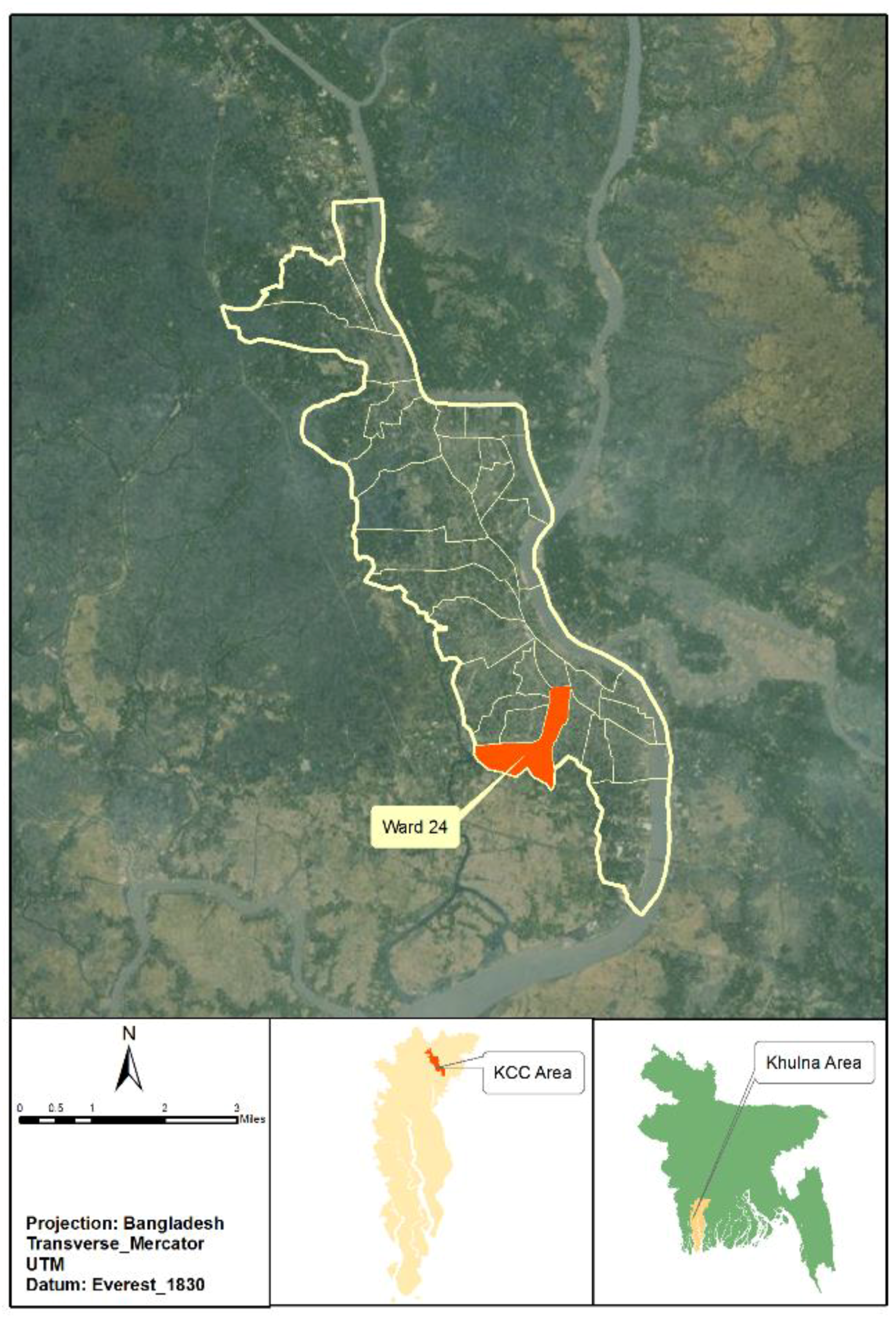
In this study, we explored one of the dense residential areas (administrative identity: Ward 24, Figure 1) of Khulna City Corporation (KCC). Ward 24 is one of the planned residential areas in Khulna City, which was designed and developed by Khulna Development Authority (KDA) in 1998 [41]. The presence of high and middle-income families had made the study area one of the major consuming residential zones in Khulna city. Moreover, a heterogenic housing pattern and a similar economic setup for individual families represents the diversified nature of household consumption. Considering these primary factors of consumption patterns, in this research, the Nirala residential area (Ward 24) has been taken as an appropriate representation of fundamental per-capita resource demand (i.e., land use, transport, food consumption, water consumption, waste generation, etc.) of middle and high-income households in Khulna city.
Stress associated with urban growth can be determined according to the methodology developed by the Global Footprint Network [42] The ecological footprint of an area comprises of six different components, i.e., cropland, grazing land, fishing ground, forest land, built-up land, and carbon uptake land footprint [2]. This study investigated the carbon emissions from the day-to-day consumption of household activities of Ward 24 by following the component-based approach, as shown in Table 1 [9]. We considered the built-up and carbon uptake land footprint (following the concepts of the Global Footprint Network) for overall footprint assessment. On the other hand, cropland, grazing land, fishing ground, forest, and built-up land [2] were taken as components of biocapacity. We compared the calculated footprint with the available biocapacity of the study area (determined from the cropland, grazing land, forest land, fishing ground, and built-up area), and thus, the stress area was quantified and visualized through mapping.
After reviewing the numerous literature on urban metabolism and ecological footprint, we developed the research hypothesis, as well as our understanding of the interaction between the urban and natural environmental, and intervention by the consumption habits of people. Accordingly, we designed a research matrix from the findings of the literature reviews by addressing the required data, methodology, data collection processes, and data sources (Table 2). We calculated household-based material consumption from the results of a questionnaire survey. We used relevant demographic data of the study area from the community series report of the Bangladesh Bureau of Statistics (BBS) to determine the sample size of the study. In this process, we projected the population of 2015 (using a polynomial growth curve based on the growth rate and trend of the several decades: 1991, 2001, and 2011), and found 35,613 as the predicted population of the study area. Subsequently, we calculated the number of households (8729) from the projected population of 2015 by considering the average household size of 4.08 [43,44]. Finally, 368 families were determined as the sample size (for a population size 8729 households with a 95% confidence level and 5% significance level, the sample size is 368 households) [45]. Then, 368 families were randomly surveyed to collect home-based material consumption. Besides, we obtained the data related to transportation characteristics (trip generation and vehicle type) through a questionnaire. In this process of the household survey before conducting the final poll, we did a pilot survey of 20 households to check the data reliability, and later, the process continued toward an extensive questionnaire survey. Following the feedback from the pilot survey, we revised the preliminary questionnaire and surveyed 368 houses based on an updated questionnaire. However, for the analysis, we considered 140 households’ responses (38.04% of the total sample size determined) with complete and adequate information. Although the sample households were randomly selected, the spatial clustering in the selection process was avoided to ensure the representation of data to a full spatial extent. Along with household surveys, we collected some relative and relevant information such as contemporary unit price of electricity (from the West Zone Power Development Board), amount of gas in a liquid petroleum gas (LPG) cylinder (from the website of Basundhara Gas Limited), current fuel and average household commodity price (from three local shops, and assumed that people buy their essential and daily commodities from nearby places) in order to calculate the household level ecological footprint. The study also used standards and conversion factors (i.e., equivalency factors, yield factors, sequestration factors, etc.), which were collected from different research agencies such as the Stockholm Environment Institute (SEI), Berkeley Institute on the Environment (BIE), Intergovernmental Panel on Climate Change (IPCC), and Global Footprint Network (GFN). We extracted the base land-use and land-cover data of the study area from the spatial database of the Khulna City Detail Area Plan (DAP, 2010). Thus, there remained a temporal gap between the collected spatial data and the present land-use of the area. We minimized this difference of land-use and land-cover data by using Landsat imagery (30 m × 30 m resolution), grid-based data input in ArcMap platform, high-resolution Quickbird (0.61 m panchromatic image), Google Earth imagery, and by visiting sample sites to cross-check the newly produced land-cover map of the study area. In this process, we used Landsat imagery and grid-based data input for the preparation of a land-use–land-cover map of study area. Quickbird and Google Earth imagery interpretations helped to derive precise information about the land use and land cover of the study area, and site visits (ground-truthing) supported the accuracy checking of the land-use and land-cover map. For ground-truthing, we visited 50 randomly selected sites that belong to different land-cover classes.
The collected data from the household survey were used to calculate the yearly material flow of the study area, and the metabolic relation regarding materials flow was established and developed in tabular form. Based on the annual material flows, sector-specific emissions were calculated (using different emission factors) and compared with the biocapacity of the area. The carbon footprint was found by summing the atmospheric emissions of carbon dioxide from the burning fossil fuels that resulted from various day-to-day consumptions such as food, water, and services (Table 1). We converted the resultant total carbon dioxide into the amount of bioproductive forest land by using a sequestration factor of forest of 1.6175 tons CO2/acre/Year [46]. This transformed amount indicates that the forest land area that would be required to store/sequester the emitted CO2 in that year. Then, the calculated area (acre) was converted into hectares, and subsequently to global hectares with the help of the equivalency factor of forest (1.26 gha/hectare) [42]. In this paper, we presented the gap between the biocapacity and footprint of household basis human consumption through mapping regarding spatial extension as a stressed area. A schematic diagram (Figure 2) presents the overall approach to attaining the desired goal of the study.
3. Ecological Footprint and Biocapacity Calculation
3.1. Built-Up Footprint
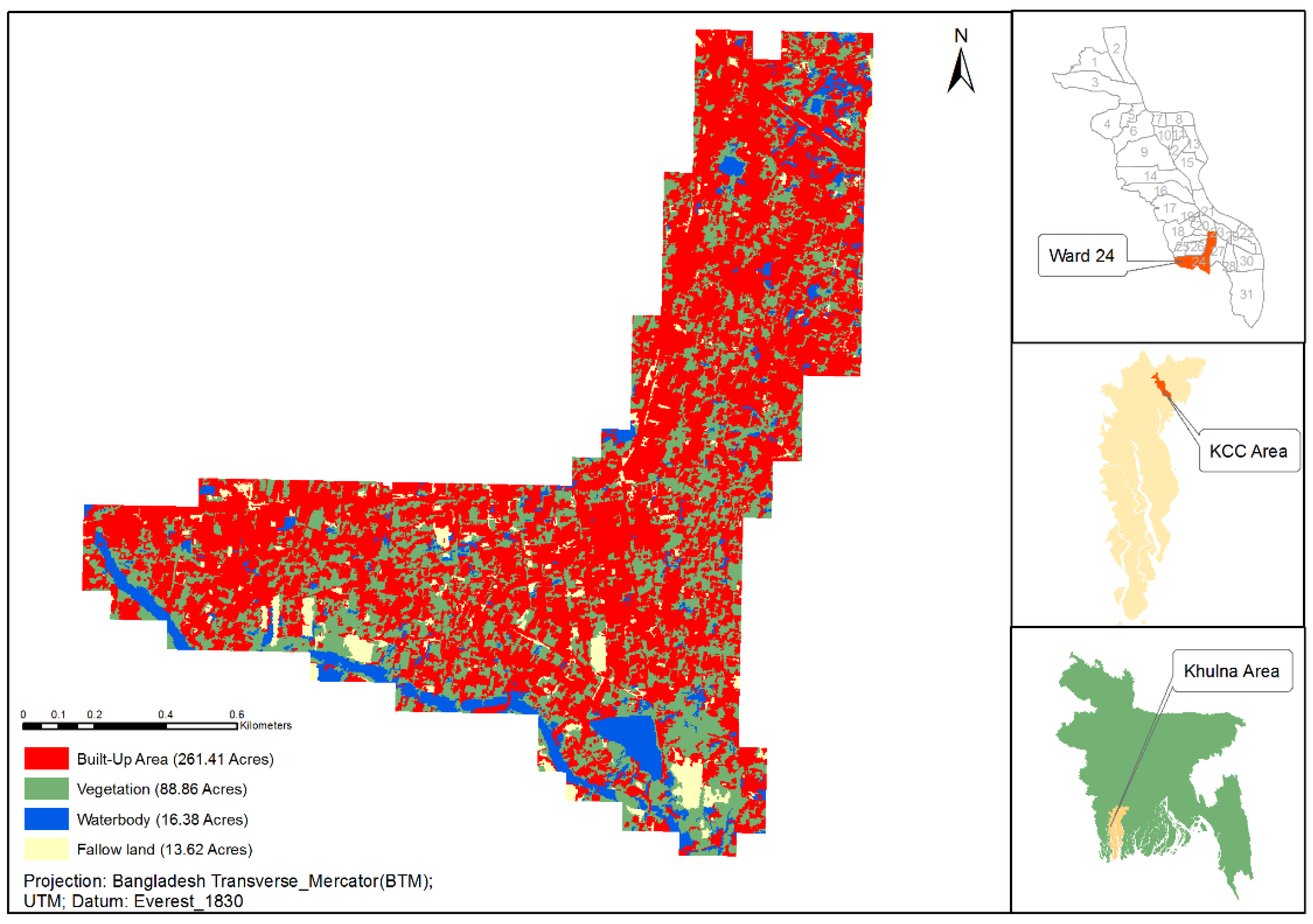
We assessed the built-up footprint based on the classified land cover of the study area into four categories (built-up, vegetation, waterbody, fallow land). In this process, we validated the detailed land-cover map with multiple references by cross-checking the land-use–land-cover map of the Detailed Area Plan (DAP) [47] of Khulna city with Quickbird imagery, Google Earth imagery, Landsat 8 imagery (30 m × 30 m pixel resolution), and by visiting the field directly. For this purpose, we downloaded freely available Landsat 8 images from the United States Geological Survey (USGS) website with no cloud coverage [48]. The whole study area was divided into a grid of 15 ft × 15 ft to ensure a readable and manageable file size (the smaller grid size produces more accurate values, but it creates a larger file). Thus, based on the purpose of the study, 15 ft × 15 ft grids (creating a 15 ft × 15 ft resolution image) were selected, and accordingly, data were cross-checked and updated to generate a precise land-cover and land-use map (Figure 3 and Figure 4).
Based on the different available methods, we performed a knowledge-based classification to attain the most updated and reliable land cover classification for the study area. A blending of complex methodology was applied to determine the built-up portion of the study area with a low level of error.
We found 261.41 acres of the total built-up area of Ward 24, and assumed this area as the stress-producing zone by reducing the biocapacity of the land. In the conversion process, it became 265.74 gha (amount of forest area needed to sequester the carbon emission) for 261.41 acres of built-up area (Figure 4).
For an accuracy assessment process, changed and unchanged pixels were cross-tabulated against the resultant images derived from the different algorithms. Each of the methods has its own advantages and disadvantages (Table 3) and it is found that knowledge-based image classification is the most effective one. In this study, we also found the similar result. To find out the overall accuracy of the different image classification methods, 50 ground training points were collected by using a handheld Global Positioning System (GPS) device. Subsequently, we calculated the overall accuracies by dividing the total number of correctly classified pixels by the total number of pixels. We estimated the exactness of the categorized images at change/no change levels. All of the points were identified, marked according to their land-cover class, and used to check the accuracy of the classified image. Amongst different classification methods, knowledge-based classification produced a more accurate result (kappa coefficient 0.91) (Table 4), as it incorporated all of the classification results, as well as a straight field investigation-based input at the pixel-level distribution of land cover of the study area.
3.2. Carbon Uptake Land for Household-Based Consumption
The amount of total carbon uptake land for the study area was estimated based on calculated carbon emissions from household consumptions. The consumable component of households according to the component approach is listed, assessed, and discussed in the subsequent sections.
3.2.1. Energy
Impacts of energy use in greenhouse gas (GHG) emissions include burning fossil fuels for transport purposes, energy generation, distribution, maintenance, etc. We calculated energy consumption in three categories for the household activity of Ward 24. They are electricity consumption, natural gas consumption, and firewood or charcoal consumption.
Electricity Consumption
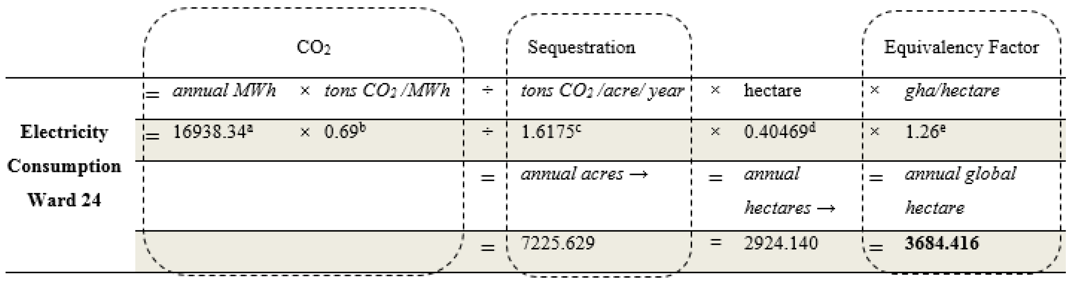
We evaluated the amount of electricity consumption from the average monthly electricity bills. During the survey, households were requested to provide an approximate amount of electricity bills by considering the seasonal variation of the summer and winter seasons. After estimating the total amount for an electricity bill in a year, we converted it into a unit of electricity consumption: MWh (megawatt per hour), with the help of the unit price of electricity, which was collected from West Zone Power Distribution Company Limited. Finally, we estimated the amount of carbon dioxide emission from each unit of MWh electricity use by using the standard value, which was collected from the Greenhouse Gas Equivalencies Calculator of the United States Environmental Protection Agency (EPA) (Figure 5).
Natural Gas Consumption
We calculated household-level gas consumption from the surveyed data on the amount, size, and price of each gas cylinder required per household per month. During the questionnaire, survey respondents were instructed to give an approximate amount by considering the seasonal variations of consumptions. We calculated the consumption of gas amount in cubic meters for a whole year from the monthly amount of total use per household. Subsequently, we transformed the annual aggregate amount (cubic meter) of gas consumption into the amount of carbon emission by multiplying standard value, which was collected from the Greenhouse Gas Equivalencies Calculator of the United States Environmental Protection Agency (EPA). Figure 6 demonstrates the calculation procedure for ecological footprint from natural gas consumption for domestic purposes.
3.2.2. Water
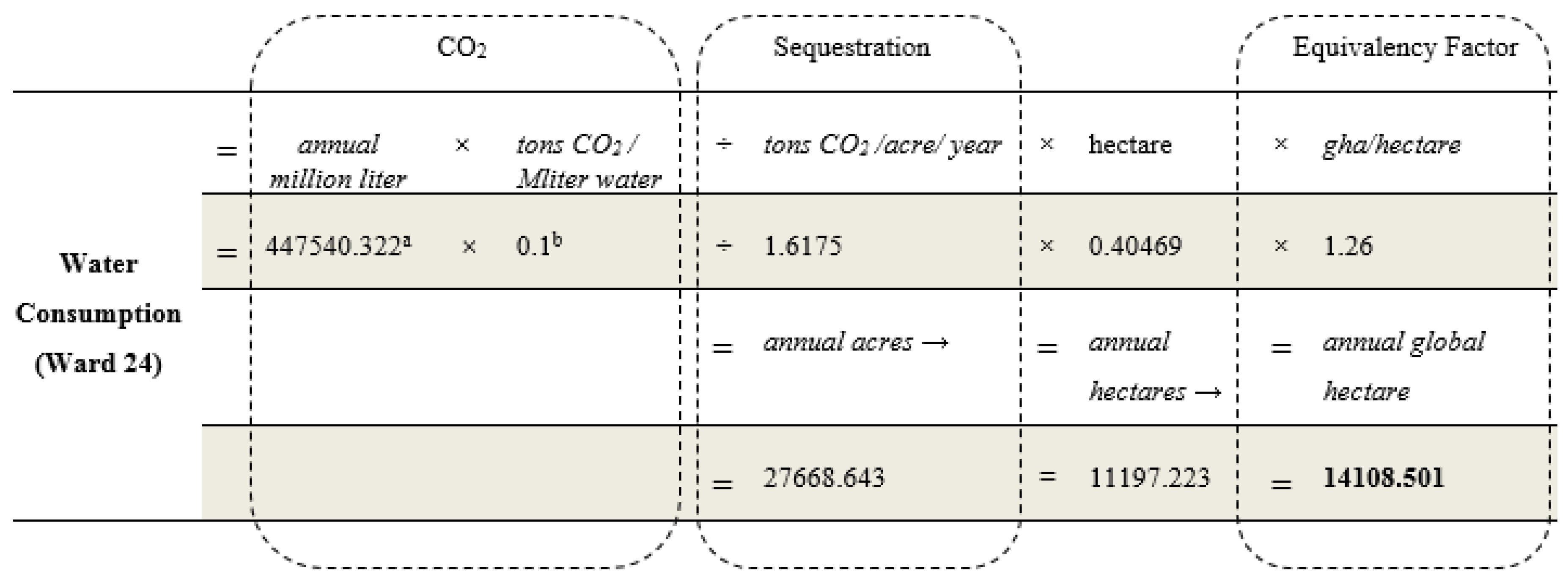
The impact of water consumption on GHG emission was not mentioned in the component method of ecological footprint assessment [9] However, in the case of some recent footprint studies [58] it has been added as a component. It includes electricity consumption, the horsepower of the pump, the size of the water tank, and sectors of water use per household. In this study, we calculated the yearly amount of water consumption from the data of water use per household per day. After deriving the total amount of consumption in millions of liters, the aggregate amount of carbon emission was estimated using the standard value of research work on southwest England by Chambers et al. (2005) [58]. However, we omitted the water consumption part when calculating the total footprint, as the study area majorly depends on the private tube wells and pumping of groundwater. Figure 7 demonstrates the calculation of the water consumption footprint. Despite the omission of water consumption, this estimation (Figure 7) is presented to give an idea of footprint based on the water demand that needs to be supported by a well-developed water supply network, treatments, and further processing.
3.2.3. Transportation
We assessed the impact of transportation on CO2 emissions under two broad categories: fuel consumption and asphalt. Initially, the emission from the transport network was estimated based on average traffic flows. However, the traffic flow-based footprint does not necessarily reflect the footprint of households in that area, as the outsiders visit and pass the zone by sharing part of the emissions. Therefore, we considered only home-based trip generation, and associated fuel consumption for the assessment of the household-based transport footprint of the study area.
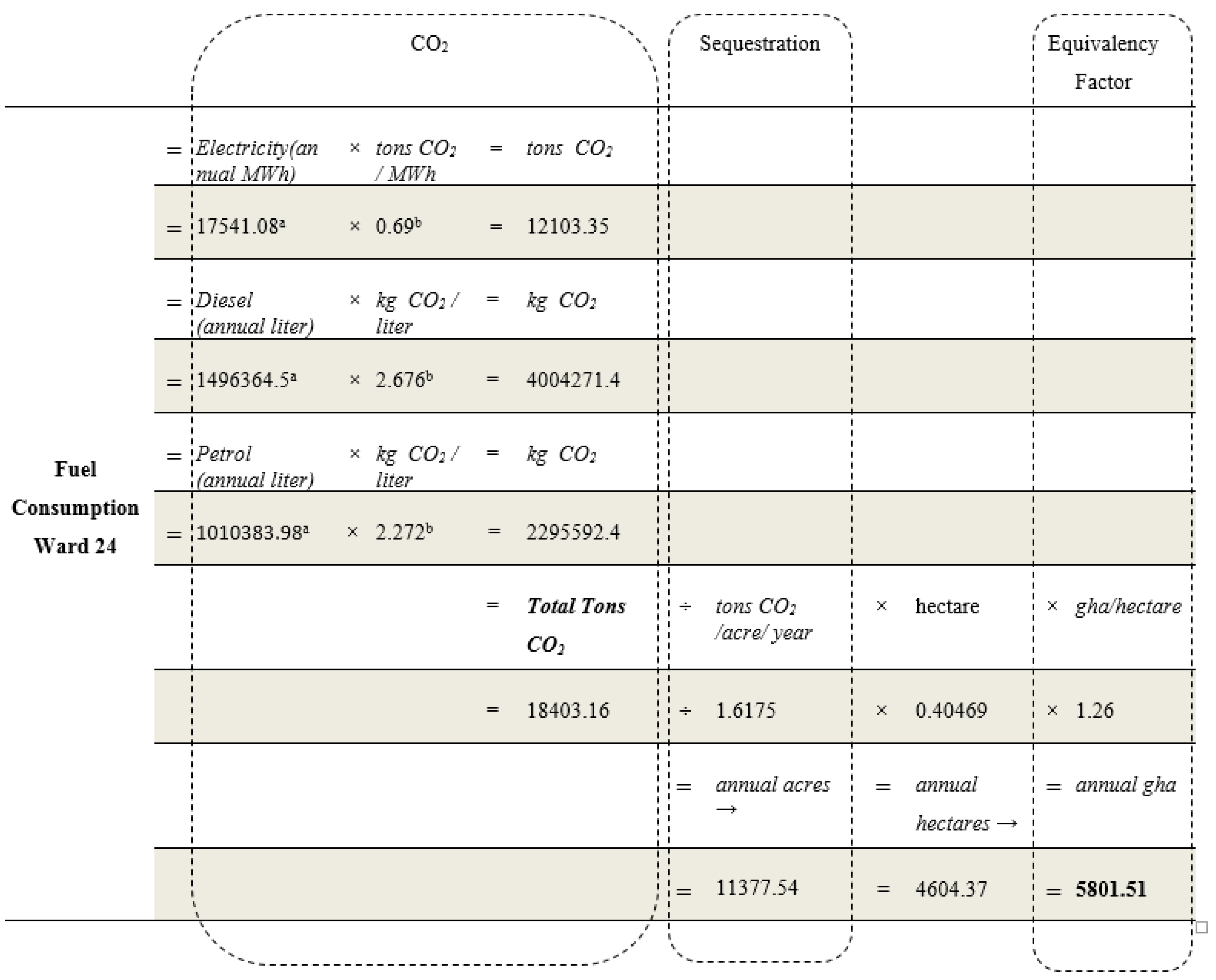
Fuel Consumption Impact
We calculated the total amount of different types of fuel consumption from the households’ daily and weekly trip generation rate, the transport mode that was used, and the modal distribution for each trip. Annual trip generation and modal distribution were calculated according to the classified uses of fuel. The number and type of vehicle, and the per-month average fuel cost of the respective mode were estimated in this process. Figure 8 presents the method of the determination (by using the unit price of each fuel type) of total annual expenditure for each type fuel on a yearly basis. Carbon emissions were calculated using the Mobile Transport–Fuel Combustion Standards for Electricity, Diesel, and Petrol, which were collected from the Greenhouse Gas Inventory Protocol Core Module Guidance [59].
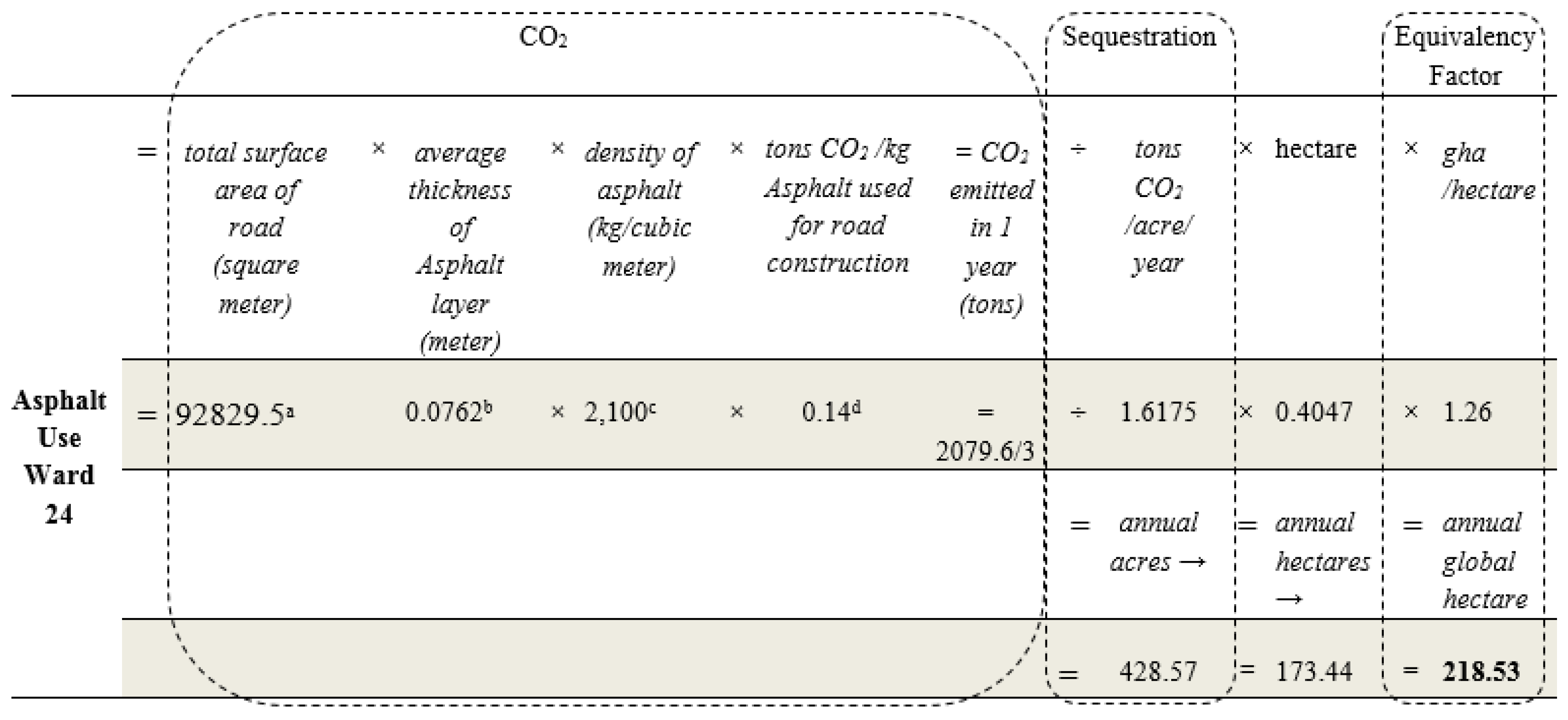
Asphalt Impact
We assessed asphalt impact in the ecological footprint of the study area from the amount of asphalt that was used during the carpeting of the road for maintenance purposes. For this purpose, the respective professionals of Khulna City Corporation were contacted to obtain the road carpeting frequency of the Ward 24 Residential areas. We were informed that the city authority did the regular carpeting in two or three-year intervals, depending on the condition of the roads. In this study, we considered three years as the time interval of the routine carpeting of roads. Accordingly, the impact of asphalt use would be one-third (1/3) of the total footprint account in a year. We extracted the whole surface area of roads from the GIS-based land-use map of Ward No. 24 of KCC (Part of DAP, KCC), and found the area of pucca (paved) road in Ward 24 was about 29.94 km, (29,945 m) and the area for Ward 24 was 92,829.5 square meters.
According to the Road Materials and Standards Study of Bangladesh (RHD, GoB, 2001), on average, a three-centimeter (depth) asphalt is used in case of traditional road maintenance in Bangladesh. Mathematically, the volume of asphalt used in each time of carpeting was determined by multiplying the total road surface area with the depth of the pavement. The density of asphalt and carbon emission per unit mass (kg) use of asphalt was collected from the Inventory of Carbon and Energy (ICE) V1.6a [61]. Subsequently, using these values, the total carbon emissions and the footprint were determined, as shown in Figure 9.
After summing up fuel consumption and asphalt impact, the transport-oriented footprint of Ward 24 became 6020.04 annual global hectares.
3.2.4. Waste
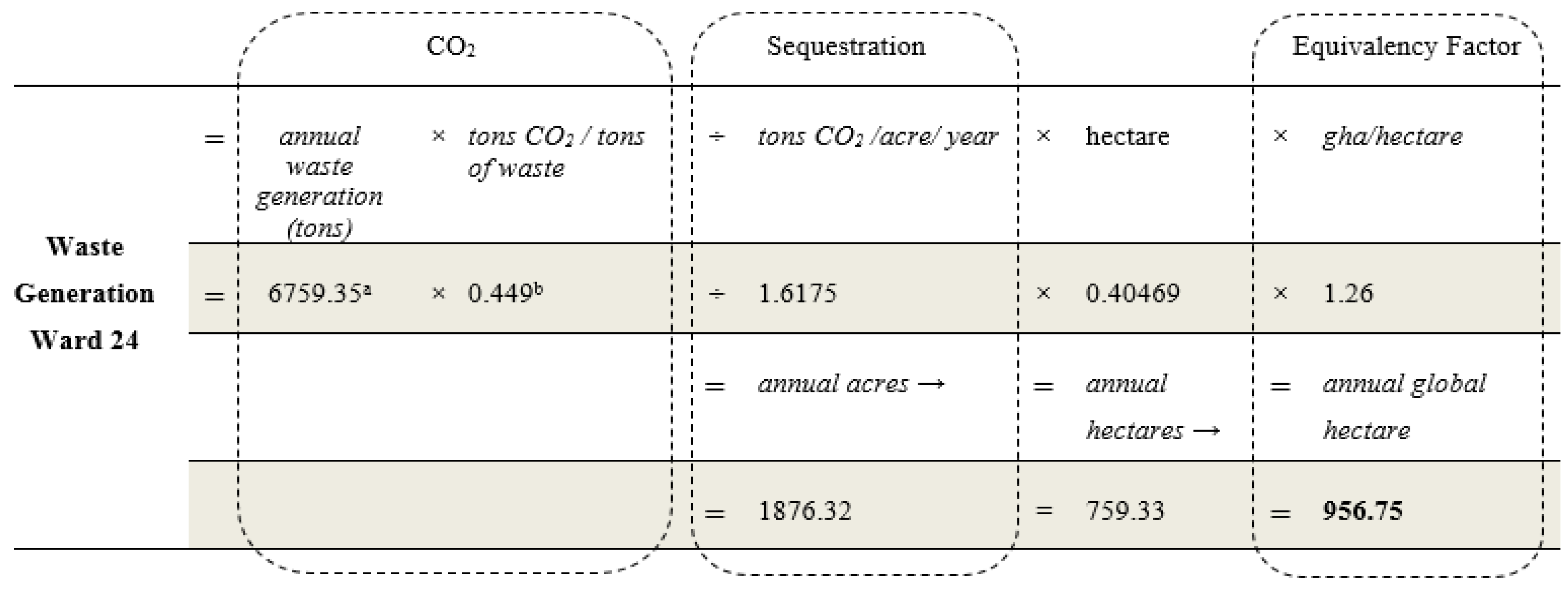
According to the methodology of the IPCC 2006 Guidelines for National Greenhouse Gas Inventories, determination of the impact of waste production in GHG emissions is a very complicated procedure [64]. To overcome this challenge, we collected the overall measurement of the bin or garbage bags, weight, and the frequency of production of the wastes per household per day. Later, following the stream of analysis, the overall waste generation and footprint of household waste were calculated for the all of the families of the study area (Figure 10).
3.2.5. Food
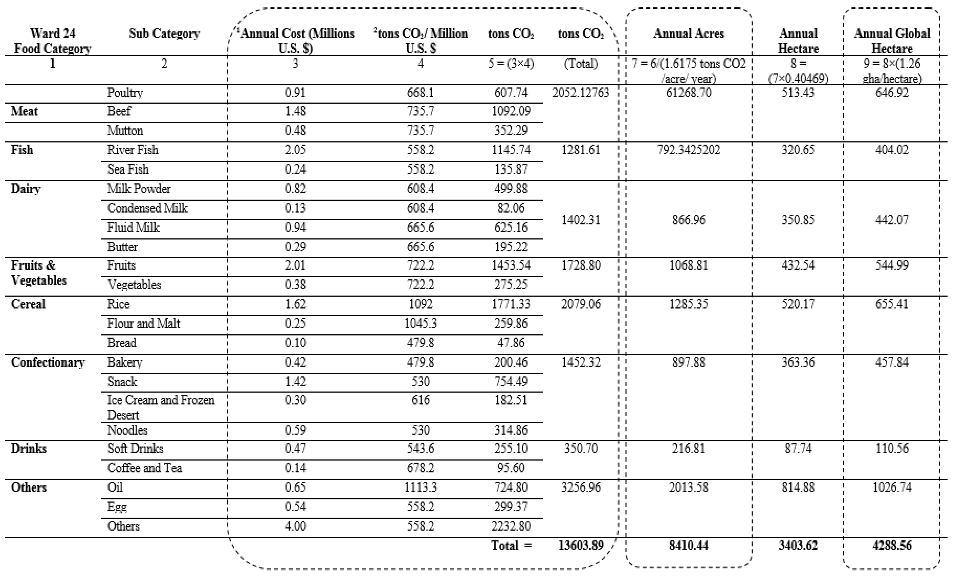
The ecological footprint of any area is profoundly influenced by the food choice behavior of the inhabitants of that area [32]. A person’s food footprint is all of the emissions that result from the production, transportation, and storage of the food that is supplied to meet their consumption needs. We assessed the impacts of food consumption on the overall footprint from the collected expenditure for food consumption at a household level based on predefined categories and subcategories. During the survey, respondents provided their choices for what they ate in a week or month for each category and subcategory of food. We used the food categories that are listed in the standards for the Economic Input–Output Life Cycle Assessment (EIO-LCA) (GHG emission values for per million United States dollars (USD) expenditure in any specific consumption category) of the Green Design Institute, Carnegie Mellon University, U.S. [66].
We converted category-wise consumption units into annual consumption, and subsequently by using the unit price (collected from a local super shop), we calculated the yearly cost of consumption in domestic (Taka) as well as million USD currency (using a stable conversion rate of 1 USD = 75 Taka [67]). Finally, by applying the GHG emission standards of the Green Design Institute, and following the EIO-LCA method, the carbon dioxide emission for each consumption category of food was calculated (Figure 11).
3.2.6. Goods
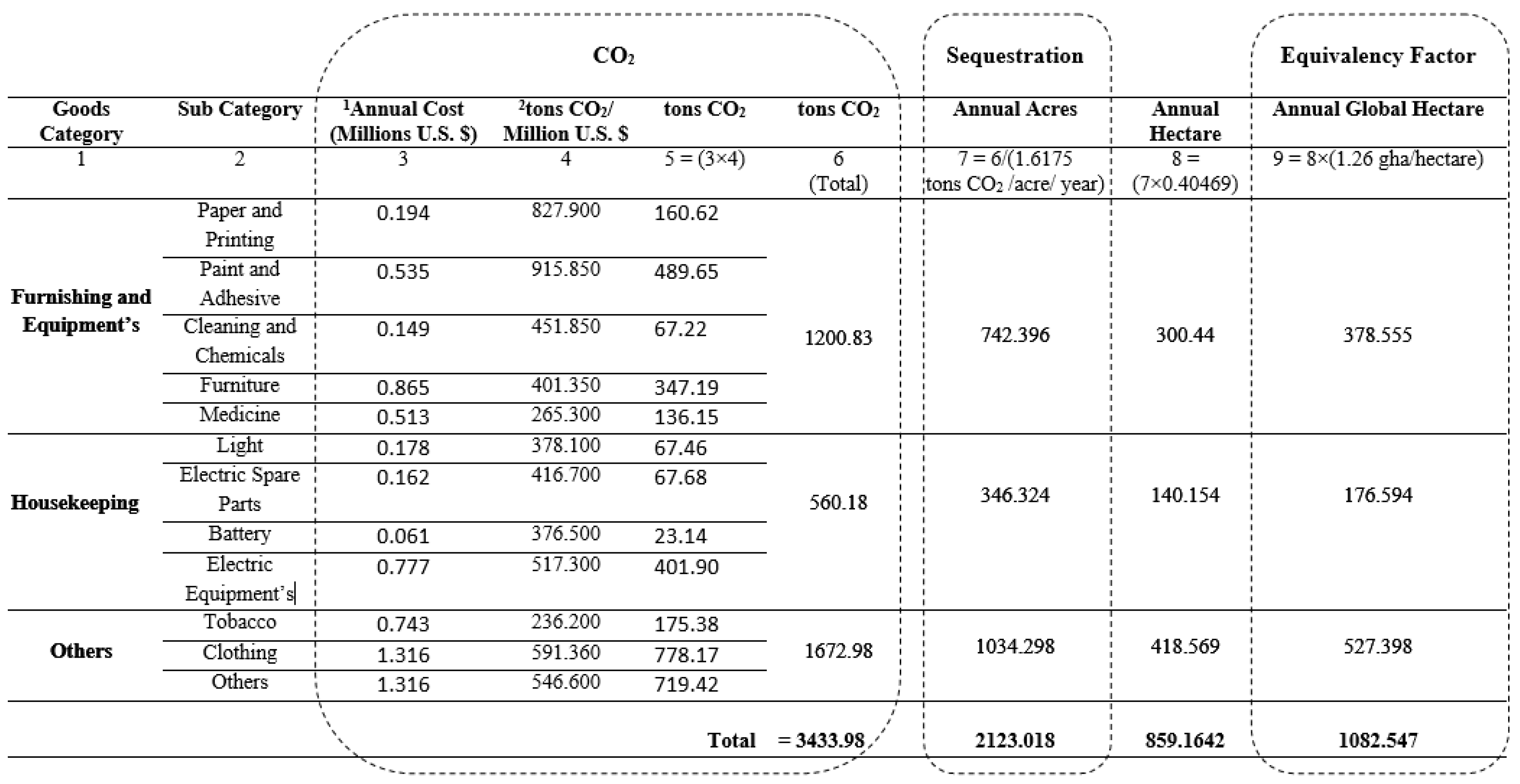
The goods consumption footprint implies GHG emissions for the consumption of things other than food and services. We categorized goods consumption under two broad classes: equipment and furnishing goods, and goods used for housekeeping activities. Subcategories of products for day-to-day use was determined based on the availability of GHG emission standards from the Green Design Institute, Carnegie Mellon University, U.S. [66]. We included the moderate numbers of the category by goods consumption, and collected monthly or yearly expenditure for those specified classes. Sequentially, by using the conversion standards, we calculated GHG emission per million of spending in each group. Finally, by dividing and multiplying the sequestration and equivalency factor, respectively, the footprint for goods consumption was calculated. Figure 12 presents the details of the calculation procedure.
3.2.7. Services
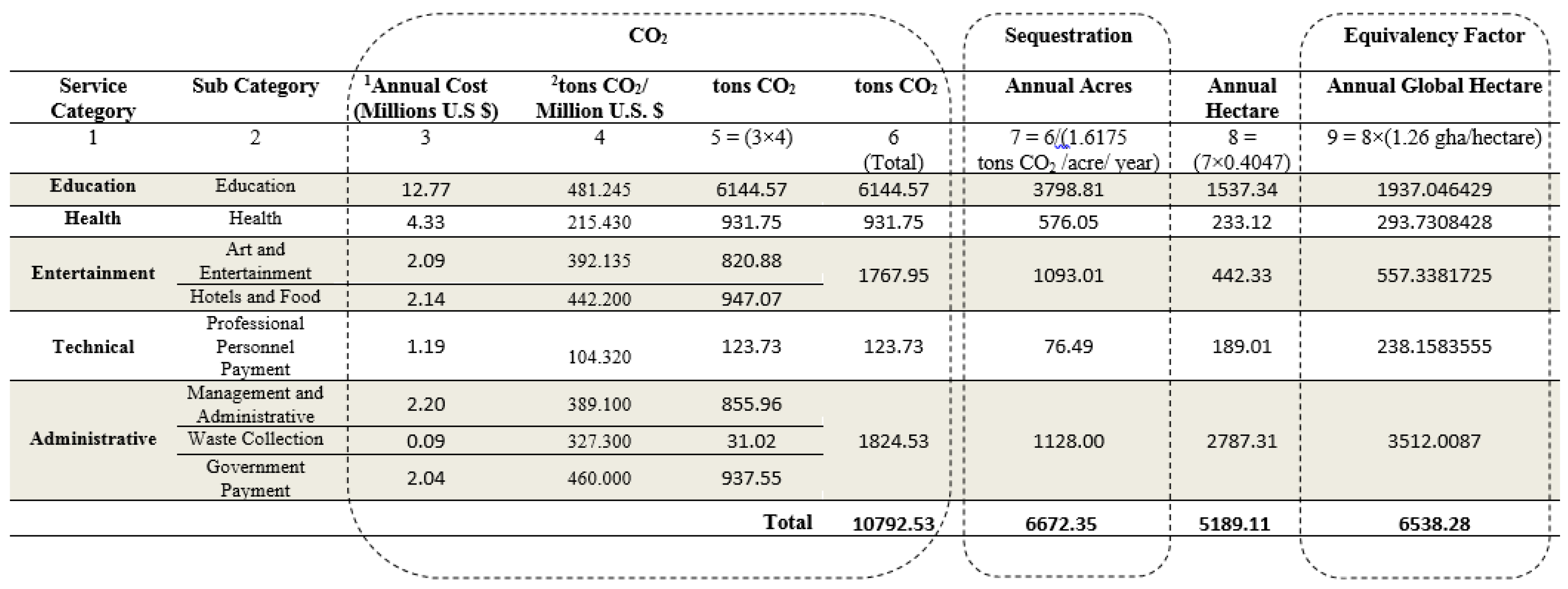
Expenditure on service activity has been found as a significant portion of most of the recent footprint studies [46]. Service activity means investment or consumption other than food and goods. It includes administrative cost, the cost of cell phone use, professional personal payment (house tutor), and similar types of fees. In this research, we assessed expenditure for service activity under four broad categories: education, health, entertainment, and technical/administrative. Subcategories were determined based on the availability of carbon emission standard values from the Green Design Institute, Carnegie Mellon University, U.S. [66], which was discussed earlier in the food and goods section. We calculated the amount of carbon emissions from the monthly or yearly expenditure by following the procedures discussed in the earlier two parts. Figure 13 presents the detailed calculation procedure for estimating the carbon emissions from different services.
3.3. Overall Footprint
The total footprint by different components of the Ward 24 (Nirala) residential area is demonstrated in Table 5. The footprint for each constituent has been illustrated in hectares, global hectares, and global hectares/capita unit.
3.4. Biocapacity
Biocapacity measures the ability of the available terrestrial and aquatic areas to provide ecological services. It also measures how much of this capacity is occupied by built-up land (infrastructure). In this study, we estimated the biocapacity of the study area based on the results of image classification. According to the author-generated knowledge-based image classification (Figure 3 and Figure 4), the study area is comprised of fallow lands, water body or fishing grounds, built-up areas, vegetation cover or forested lands (all of the vegetation cover was assumed as forested land). To calculate the biocapacity of the study area, all of the water bodies were considered as a fishing ground, and the yield factor was assumed to be equal to the national level. By doing this, the overestimation of biocapacity was ensured to meet the principles of footprint and biocapacity calculation. On the other hand, the biocapacity of the built-up area is equal to its footprint, and it is also assumed that built-up land occupies what would previously have been cropland [69]. Since both the footprint and the biocapacity of the built-up area estimate the amount of bioproductivity that is lost to encroachment by physical infrastructure, in this study, the yield factor of cropland was considered as the substitution to calculate the biocapacity of the built-up area; thus, the whole study area was considered a bioproductive land [69]. Nonproductive or protected area is not a concern of biocapacity calculation in this study, as there is no such area. Moreover, nonproductive lands are ignored in biocapacity calculation, since their production is too widespread to be directly harvested, and is negligible in quantity.
For biocapacity calculation, we used the formula that has been developed by the Global Footprint Network [42]:
where, = area available for a given land-use type, and = yield and equivalence factor, respectively, for each area, year, and land-use type.
4. Results and Discussion
This study has developed the scenario of household consumption from an ecological footprint perspective by demonstrating the relevant facts and figures at a local level. We have found that the study area is experiencing the overshooting condition (stressing), as the total ecological footprint (25,502.54 gha or 255,025,400 square meters) of Ward 24 is far greater than the calculated biocapacity (510.12 gha or 5,101,230 square meters). This situation is indicating that the amounts of household resource consumption in the study area are exceeding the calculated biocapacity by 24,992.42 gha (25,502.54 gha versus 510.12 gha), which is creating environmental stress to the surrounding areas (). A similar situation is observable when we compare the per-capita footprint and biocapacity of the study area. The per-capita footprint of Ward 24 is 0.7161 gha (Table 5) (food + goods + services + transport + energy + waste + built-up land), while the per capita supply of biocapacity is only 0.0144 gha (Table 6) (vegetation cover + waterbody + built-up land). Comparing these two figures, it is found that the per-capita demand of ecological footprint for household consumption in Ward 24 exceeds its biocapacity (biocapacity) by 49.73 times, even if we consider the built-up area as a bioproductive land (the biocapacity of the built-up area is calculated considering it as cropland). We get a clearer picture of the stress situation by comparing the available land mass (380.27 acres or 154 hectares) of the study area with the extra demanded land area (24,992.42 gha) for supporting the present level of resource consumption and waste sequestration services. This additional demand of land area indicates that Ward 24 will require an area that is 162 times larger than at present to meet and support the present level of household consumption. The situation is more alarming if we only consider the vegetation and water body land covers as bioproductive areas. The biocapacity of the study area is only 20.79 gha (Table 7) if we ignore the biocapacity of the built-up area, which is only 13.5% of the total available land area. The study area comprises only 0.62% of the extra land area to support the annual consumption by the inhabitants (Table 7).
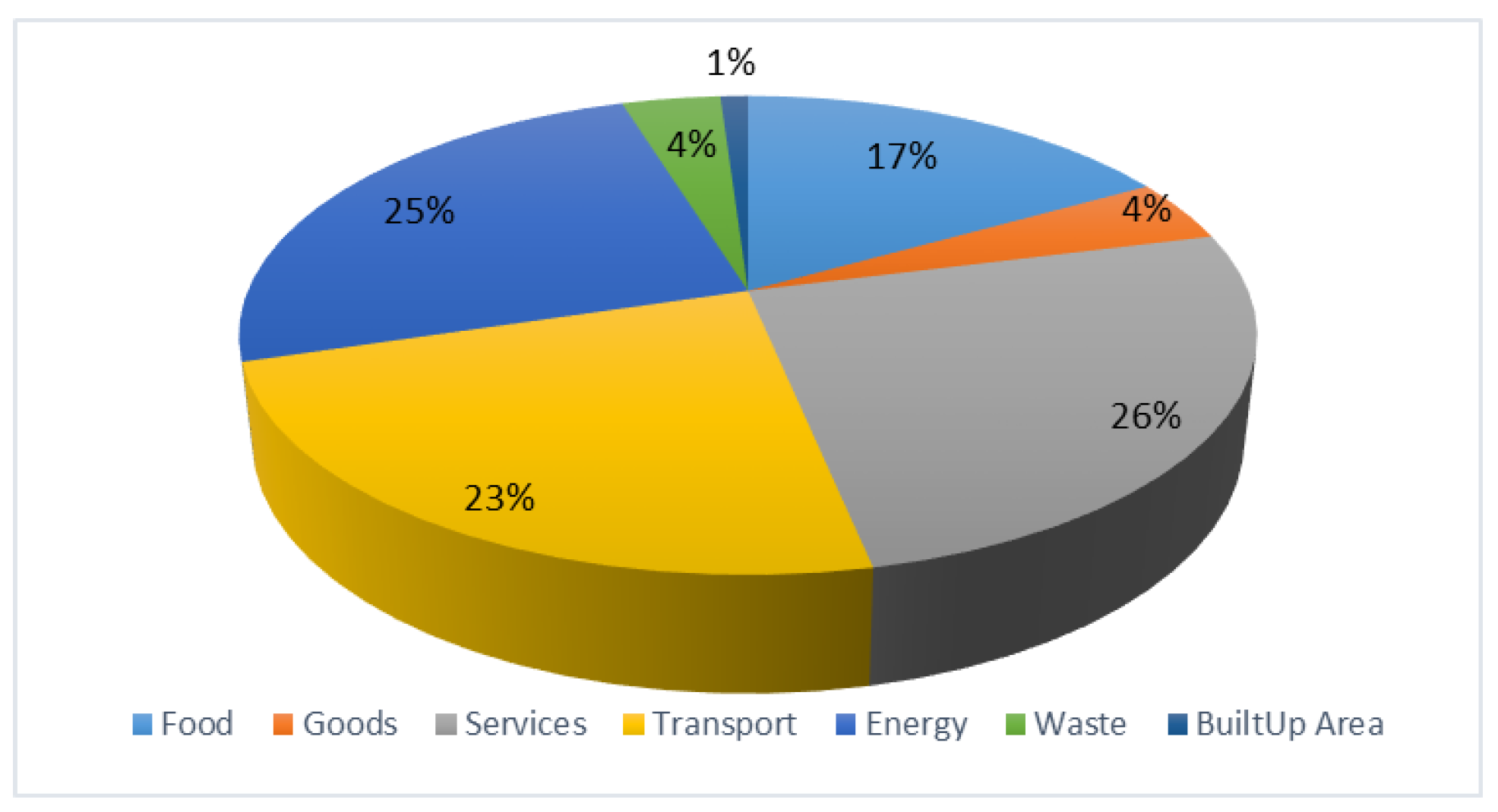
Upon comparing these figures with the per capita ecological deficit at the global and national level, the sustainability concern of the household consumption of the study area is also under threat (Figure 14). At the global and national scale, the per-capita ecological deficit is 1.1 gha and 0.3 gha, respectively. The per capita deficit (0.70 gha) of the study area is greater than the national level deficit (0.3 gha). This deficiency is signaling the overconsumption and unplanned materials flow in different sectors of the study area. The sector-specific findings of this study clearly depict the sharing of this additional consumption at the household level. The study identified the various sizes of ecological footprint components, which directly provide the facts and figures to the government as well as policymakers to focus on the area and strategies to reduce the overall footprint. As this study applied the component method and relied on the primary data of household consumption, the estimation approach is direct compared with the studies that relied on the power of other explanatory variables for calculating ecological footprint, such as per capita income [32], per capita expenditure [72,73], population density, and pollutant emission intensity. In this regard, this study methodologically produced a better approximation of the estimated ecological footprint and represented the pathways of addressing the problem of household consumption and associated ecological stress by thinking globally and acting locally. The study has found that the service (26%), energy (25%), and transport (23%) sectors are the three major contributors of the footprint at the individual level (Figure 15). The footprint from food consumption, waste generation, and other goods consumption is relatively low, which suggests that the service, energy, and transport sectors should receive proper policy intervention for reducing the footprint, as well as reducing the ecological deficit. However, reducing consumption or intervening in the consumption pattern through policy options is not a straightforward task, due to some interrelated effects. Moreover, the increased rate of consumption in different sectors is an inevitable situation with the increase in household income. Due to this dynamism of consumption patterns, direct intervention to reduce or regulate consumption patterns is not a realistic option to address sustainability concerns in urban life. Instead of an immediate and direct response, the policy options that promote indirect restrictions regarding demand management are more pragmatic.
For example, in the case of the transportation system, there is no alternative other than increasing the mobility of a livable urban environment. In the modern transportation framework, mobility comes through the consumption of more fossils, which are increasing the footprint at the local as well as the national level. There is limited scope to regulate the movement of people directly, as it goes against the freedom of choice at the individual level. In this case, policymakers should adopt restrictions in such a way that can modify peoples’ demand indirectly and consequently reduce the transport footprint. Travel demand management strategies can play a useful role in achieving this. The footprint calculation and identification of specific sectors can provide corroborative components in this process of indirect policy intervention.
From a sustainability perspective, planners should promote demand management strategies with the target of limiting the footprint of different sectors.
It is essential to visualize the nature of the problem spatially for policy formulation and intervention. Visualization through maps and visual images from GIS expressing footprint measurement and comparisons enable local policy planners and community representatives to communicate with stakeholders and bring the issues of sustainability in resources consumption to the table for negotiation [32]. The use of ecological footprint analysis is a challenging visual tool, particularly when it is applied for comparisons between jurisdictions. Despite this challenge, the representation of the ecological footprint is used as a way of measuring and demonstrating the extension of ecological stress impacts far beyond the built areas of cities [74]. The main challenge arises in this representation process from the area where the footprint of an area occurs. In the spatial representation process, the consideration of footprint as a single factor generates disproportionate results, as the footprint of an area is represented by using the surrounding land areas [74] In this study, we have overcome this limitation of disproportionate representation by considering the ecological footprint and biocapacity on the same map. We presented the spatial extension of the ecological footprint by subtracting the biocapacity, which is a simple but unique approach to address the issue of the disproportionate representation of the footprint. This study has presented a way to visualize the ecological footprint in a proportionate way in terms of local environmental stress by considering the total ecological footprint and biocapacity. For this purpose, we represented the comparative picture of ecological footprint and biocapacity by taking the reference of the study area within the administrative boundary. In Figure 16, the spatial extent of the calculated demand regarding the land mass area is represented to visualize the situation.
In the depicted scale of the map, it is expressed that the study area with a population size of 35,613 and a per capita 0.716 gha footprint is demanding a large area size from its surroundings beyond its boundary. Regarding externalities, the consumption pattern of the study area is creating impacts on the natural resources of the surrounding areas. The spatial extent of the footprint is showing an extraordinarily extensive area beyond the actual study area, as the footprint is calculated based on the annual consumption and represented through a single spatial extent. On the other hand, the biocapacity is illustrated as fixed, as it takes time to produce an individual good or service depending on the production capacity and yield factors of the land.
This spatial representation is a helpful tool to consider the issue of environmental justice in planning and policy development with the harmony of sustainability. From the spatial illustration, it is understandable that at the local scale, the consumption habits of one area’s residents are taking the share of the natural resources of other areas of development. This spatial representation is especially helpful when regarding the issue of negotiation among different interest groups with the individual entity. Notably, it is also supportive in cases of formulating regulations by which it is possible to reduce the externalities of one community in other communities. For example, by fixing compensation or tax to reduce the externalities of one community to another community, this analytical tool can play a vital role in the primary negotiation process. Notably, in a robust democratic environment, the issue of environmental justice should be a matter of practice at the local level, with the active participation of local people and local government. This spatial representation process at the local scale will provide a window to think locally by using the global perspective of the footprint.
5. Conclusions
The study shows the environmental stress due to household-based consumption in Ward 24. The study followed an approach under which mapping a representation of the exerted pressure in relation to the biocapacity and the footprint was developed to visualize the spatial extent of the problem. The resulted outcome of the analysis shows that the significant contributors to environmental stress are transport, service, and the energy footprint. On the other hand, the biocapacity of the study area is very low in comparison to the footprint that results from the low availability of cultivable lands and dense urbanization. Ecological stress assessment and visualization can find out the gaps in an area that seems to be entirely in good condition regarding resource consumption. By following this, we can find out how much an area depends on its surrounding natural environment for the consumption habits of its residents. This process illustrates how many resources are available, and how rapidly human consumption habits are depleting them. It is a helpful tool to provide a measurement scale at a spatial level for planners, ecologists, and environmentalists to plan an area in a more sustainable way with the available resources. Besides, from an environmental judgment perspective, the findings of this study can be applicable in negotiations to develop an appropriate policy for ensuring sustainability in the process of urbanization. Notably, this study is also suitable for depicting the reciprocal influence scenario of one area’s consumption in other areas.
The study has some limitations. Firstly, regarding the spatial resolution of images, the study has scope to improve. Analysis of the images with small spatial resolution can produce more accurate results than what we have found. Secondly, the methodology of this research is not limited to improve further, as yearly basis data at the community level is yet to be available in Bangladesh on such issues. Moreover, the different factors that we used for the study purposes can be modified and customized as per the context and characteristics of the area. The refinement of the various conversions will provide a more accurate picture than it has already found in this study. The service footprint calculation in particular should be considered by focusing on local practices, rather than by applying the factors from previous studies. Thirdly, in the process of food categorization and footprint calculation, we tried to cover the maximum numbers of food in each different consumption category. However, this was not possible due to the absence of the standards, and the vast sociocultural differences between the study area and other countries. The correction of this limitation would demand rigorous data collection that was scaled down to the local level, which was beyond the scope of this study. However, this research has greater potentiality if conducted on a larger scale (city/regional/national scale). It can be used to formulate policy and delineate a city-scale land-use–land cover restrictions, as well as add a new dimension in the valuation process of different ecosystem services. Especially regarding evaluating the ecosystem services at the city scale, this study approach can be considered for trading off the ecosystem valuation of one area with another area, depending on their area of influence. This is only possible by depicting the spatial representation of the stress scenario of an ecological footprint. Considering future pressure on biocapacity as the global population continues to expand, and as the demand for resource constraints may become more prevalent, paying attention to biocapacity and ecological footprint at the spatial level can become an essential strategy for local and national government to increase the practice of sustainability in their planning and policy intervention process. The proportionate approach of representing the ecological footprint and biocapacity of this study can be the basis of incorporating the spatial phenomenon in the more wider extent of ecological accounting, as well as planning and policy intervention at the local and national levels.
Author Contributions
Md. Shakil Khan wrote the first draft of this paper. He processed the survey data and performed the required analysis by using the spreadsheet, GIS and RS softwares. Muhammad Salaha Uddin worked in the research design phase and supervised the whole study from data collection to analysis. He also worked on the later versions of the paper and addressed the comments of the reviewers.
Funding
This research received no external funding.
Acknowledgments
We would like to thank the undergraduate students for their hard works during the primary data collection process. We would also like to give our heartful thank to the three anonymous reviewers for their insightful and scholastic suggestions which help us to upgrade this paper. Special thanks to the Department of Urban and Regional Planning, Khulna University of Engineering and Technology for providing the support of license software and lab facilities during this study.
Conflicts of Interest
The authors declare no conflicts of interest.
References
- Moore, J.; Kissinger, M.; Rees, W.E. An urban metabolism and ecological footprint assessment of Metro Vancouver. J. Environ. Manag. 2013, 124, 51–61. [Google Scholar] [CrossRef] [PubMed]
- Shakil, S.H.; Kuhu, N.N.; Rahman, R.; Islam, I. Carbon Emission from Domestic Level Consumption: Ecological Footprint Account of Dhanmondi Residential Area, Dhaka, Bangladesh—A Case Study. Aust. J. Basic Appl. Sci. 2014, 8, 265–276. [Google Scholar]
- Hart, S.L. A natural-resource-based view of the firm. Acad. Manag. Rev. 1995, 20, 986–1014. [Google Scholar] [CrossRef]
- Khamis, A. Developing a Typology of Urban Resource Consumption. In Proceedings of the 1st Civil and Environmental Engineering Student Conference, London, UK, 25–26 June 2012. [Google Scholar]
- Hecht, R.; Kunze, C.; Hahmann, S. Measuring Completeness of Building Footprints in OpenStreetMap over Space and Time. ISPRS Int. J. Geo-Inf. 2013, 2, 1066–1091. [Google Scholar] [CrossRef] [Green Version]
- Spiller, M.; Agudelo, C. Mapping Diversity of Urban Metabolic Functions—A Planning Approach for More Resilient Cities. 2011. Available online: http://www.researchgate.net/profile/Marc_Spiller/publication/263776192_Mapping_diversity_of_urban_metabolic_functions__a_planning_approach_for_circular_urban_metabolism/links/00b4953be4885cee00000000.pdf (accessed on 23 March 2015).
- Rees, W.E.; Bunting, T.; Filion, P.; Walker, R. Getting Serious about Urban Sustainability: Eco-Footprints and the Vulnerability of 21st-Century Cities; Springer: Toronto, ON, Canada, 2010; Available online: http://whatcom.wsu.edu/carbonmasters/documents/UrbSustGetSeriousC5_0509.pdf (accessed on 3 March 2015).
- United Nations, Department of Economic and Social Affairs & Population Division. World Urbanization Prospects: The 2014 Revision: Highlights; Undesapd; Department of Economic and Social Affairs, United Nations: New York, NY, USA, 2014. [Google Scholar]
- Barrett, J.; Vallack, H.; Jones, A.; Haq, G. A Material Flow Analysis and Ecological Footprint of York; Stockholm Environment Institute: Stockholm, Sweden, 2002; Available online: https://www.researchgate.net/profile/Gary_Haq/publication/257494298_A_Material_Flow_Analysis_and_Ecological_Footprint_of_York/links/02e7e525555fbc95ab000000.pdf (accessed on 2 March 2015).
- Meng, F.; Liu, G.; Yang, Z.; Casazza, M.; Cui, S.; Ulgiati, S. Energy efficiency of urban transportation system in Xiamen, China. An integrated approach. Appl. Energy 2017, 186, 234–248. [Google Scholar] [CrossRef]
- Dewulf, J.; Van Langenhove, H. Exergetic material input per unit of service (EMIPS) for the assessment of resource productivity of transport commodities. Resour. Conserv. Recycl. 2003, 38, 161–174. [Google Scholar] [CrossRef]
- Chen, W.; Liu, W.; Geng, Y.; Brown, M.T.; Gao, C.; Wu, R. Recent progress on energy research: A bibliometric analysis. Renew. Sustain. Energy Rev. 2017, 73, 1051–1060. [Google Scholar] [CrossRef]
- Cooney, G.; Hawkins, T.R.; Marriott, J. Life Cycle Assessment of Diesel and Electric Public Transportation Buses: LCA of Diesel and Electric Buses. J. Ind. Ecol. 2013. [Google Scholar] [CrossRef]
- Facanha, C.; Horvath, A. Evaluation of Life-Cycle Air Emission Factors of Freight Transportation. Environ. Sci. Technol. 2007, 41, 7138–7144. [Google Scholar] [CrossRef] [PubMed]
- Hawkins, T.R.; Singh, B.; Majeau-Bettez, G.; Strømman, A.H. Comparative Environmental Life Cycle Assessment of Conventional and Electric Vehicles: LCA of Conventional and Electric Vehicles. J. Ind. Ecol. 2013, 17, 53–64. [Google Scholar] [CrossRef]
- Nanaki, E.A.; Koroneos, C.J.; Roset, J.; Susca, T.; Christensen, T.H.; De Gregorio Hurtado, S.; López-Jiménez, P.A. Environmental assessment of 9 European public bus transportation systems. Sustain. Cities Soc. 2017, 28, 42–52. [Google Scholar] [CrossRef]
- Park, Y.S.; Egilmez, G.; Kucukvar, M. A Novel Life Cycle-based Principal Component Analysis Framework for Eco-efficiency Analysis: Case of the United States Manufacturing and Transportation Nexus. J. Clean. Prod. 2015, 92, 327–342. [Google Scholar] [CrossRef]
- Chester, M.V.; Horvath, A.; Madanat, S. Comparison of life-cycle energy and emissions footprints of passenger transportation in metropolitan regions. Atmos. Environ. 2010, 44, 1071–1079. [Google Scholar] [CrossRef]
- Egilmez, G.; Park, Y.S. Transportation-related carbon, energy and water footprint analysis of U.S. manufacturing: An eco-efficiency assessment. Transp. Res. Part D Transp. Environ. 2014, 32, 143–159. [Google Scholar] [CrossRef]
- Robinson, O.J.; Tewkesbury, A.; Kemp, S.; Williams, I.D. Towards a universal carbon footprint standard: A case study of carbon management at universities. J. Clean. Prod. 2017. [Google Scholar] [CrossRef]
- Schanes, K.; Giljum, S.; Hertwich, E. Low carbon lifestyles: A framework to structure consumption strategies and options to reduce carbon footprints. J. Clean. Prod. 2016, 139, 1033–1043. [Google Scholar] [CrossRef]
- Chrysoulakis, N. Urban metabolism and resource optimization in the urban fabric: The BRIDGE methodology. Proc. EnviroInfo2008 Environ. Inform. Ind. Ecol. 2008, 1, 301e309. [Google Scholar]
- Goldstein, B.; Birkved, M.; Quitzau, M.-B.; Hauschild, M. Quantification of urban metabolism through coupling with the life cycle assessment framework: Concept development and case study. Environ. Res. Lett. 2013, 8, 035024. [Google Scholar] [CrossRef]
- Guo, Z.; Hu, D.; Zhang, F.; Huang, G.; Xiao, Q. An integrated material metabolism model for stocks of urban road system in Beijing, China. Sci. Total Environ. 2014, 470–471, 883–894. [Google Scholar] [CrossRef] [PubMed]
- Kennedy, C.; Pincetl, S.; Bunje, P. The study of urban metabolism and its applications to urban planning and design. Environ. Pollut. 2011, 159, 1965–1973. [Google Scholar] [CrossRef] [PubMed]
- Mutel, C.L.; Pfister, S.; Hellweg, S. GIS-Based Regionalized Life Cycle Assessment: How Big Is Small Enough? Methodology and Case Study of Electricity Generation. Environ. Sci. Technol. 2012, 46, 1096–1103. [Google Scholar] [CrossRef] [PubMed]
- Wang, X.; Shi, X.Q. A review of industrial ecology based on GIS. Shengtai Xuebao/Acta Ecol. Sin. 2017, 37, 1346–1357. [Google Scholar] [CrossRef]
- Xia, L.; Zhang, Y.; Wu, Q.; Liu, L. Analysis of the ecological relationships of urban carbon metabolism based on the eight nodes spatial network model. J. Clean. Prod. 2017, 140, 1644–1651. [Google Scholar] [CrossRef]
- Geyer, R.; Stoms, D.M.; Lindner, J.P.; Davis, F.W.; Wittstock, B. Coupling GIS and LCA for biodiversity assessments of land use: Part 1: Inventory modeling. Int. J. Life Cycle Assess. 2010, 15, 454–467. [Google Scholar] [CrossRef]
- Hiloidhari, M.; Baruah, D.C.; Singh, A.; Kataki, S.; Medhi, K.; Kumari, S.; Ramachandra, T.V.; Jenkins, B.M.; Thakur, I.S. Emerging role of Geographical Information System (GIS), Life Cycle Assessment (LCA) and spatial LCA (GIS-LCA) in sustainable bioenergy planning. Bioresour. Technol. 2017. [Google Scholar] [CrossRef] [PubMed]
- Wackernagel, M.; Rees, W. Our Ecological Footprint: Reducing Human Impact on the Earth; New Society Publishers: Gabriola, BC, Canada, 1998; Available online: https://books.google.co.uk/books?hl=en&lr=&id=WVNEAQAAQBAJ&oi=fnd&pg=PR9&dq=ecological+footprint+and+climate+change&ots=VkVR7MpTJm&sig=ylImaW64ZbS0CWxM0CxC4dZeqko (accessed on 15 March 2015).
- Kuzyk, L.W. Ecological and carbon footprint by consumption and income in GIS. Int. J. Justice Sustain. 2011, 16, 871–886. [Google Scholar]
- Matthew, H.; Connolly, R.R. Estimating Residential Carbon Footprints for an American City. Int. J. Appl. Geospat. Res. 2012, 3, 103–122. [Google Scholar]
- Klinsky, S.; Sieber, R.; Meredith, T. Connecting local to global: Geographic information systems and ecological footprints as tools for sustainability. Prof. Geogr. 2010, 62, 84–102. [Google Scholar] [CrossRef]
- Aminuzzaman, S.M. Environment policy of Bangladesh: A case study of an ambitious policy with implementation snag. In Proceedings of the South Asia Climate Change Forum, Melbourne, Australia, 5–9 July 2010; Volume 59. Available online: http://gsdl.ewubd.edu/greenstone/collect/admin-mprhgdco/index/assoc/HASHa973.dir/P0200.pdf (accessed on 23 March 2015).
- Noss, R.F.; LaRoe, E.T.; Scott, J.M. Endangered Ecosystems of the United States: A Preliminary Assessment of Loss and Degradation; US Department of the Interior, National Biological Service: Washington, DC, USA, 1995; Volume 28. Available online: http://biology.usgs.gov/pubs/ecosys.htm (accessed on 26 March 2015).
- Tockner, K.; Bunn, S.E.; Gordon, C.; Naiman, R.J.; Quinn, G.P.; Stanford, J.A. 4 Á Floodplains: Critically Threatened Ecosystems. 2008. Available online: http://www.researchgate.net/profile/Klement_Tockner3/publication/29469521_Flood_plains_Critically_threatened_ecosystems/links/02e7e5362727ab2e83000000.pdf (accessed on 27 March 2015).
- Haque, M.M.; Ahmed, F.; Anam, S.; Kabir, M.R. Future Population Projection of Bangladesh by Growth Rate Modeling Using Logistic Population Model. Ann. Pure Appl. Math. 2012, 1, 192–202. [Google Scholar]
- Streatfield, P.K.; Karar, Z.A. Population challenges for Bangladesh in the coming decades. J. Health Popul. Nutr. 2008, 26, 261. [Google Scholar] [CrossRef] [PubMed]
- Asaduzzaman, M. Frontiers of change in rural Bangladesh: Natural resources and sustainable livelihoods. In Hands Not Land: How Livelihoods Are Changing in Rural Bangladesh; Department for International Development (DFID): Dhaka, Bangladesh, 2002; pp. 65–70. [Google Scholar]
- Kumar, U.; Alam, M.; Rahman, R.; Mondal, S.; Huq, H. Water Security in Peri-Urban Khulna: Adapting to Climate Change and Urbanization. Peri-Urban Water Security Discussion Paper Series, Paper 2. 2011. Available online: http://saciwaters.org/periurban/2%20idrc%20periurban%20report.pdf (accessed on 13 April 2015).
- Ewing, B.; Reed, A.; Galli, A.; Kitzes, J.; Wackernagel, M. Calculation Methodology for the National Footprint Accounts, 2010 ed.; Global Footprint Network: Oakland, CA, USA, 2010. [Google Scholar]
- Bangladesh Bureau of Statistics (BBS). Statistical Yearbook of Bangladesh, Bangladesh Bureau of Statistics (BBS); Ministry of Planning, Government of the People’s Republic of Bangladesh: Dhaka, Bangladesh, 2001.
- Bangladesh Bureau of Statistics (BBS). Statistical Yearbook of Bangladesh, Bangladesh Bureau of Statistics (BBS); Ministry of Planning, Government of the People’s Republic of Bangladesh: Dhaka, Bangladesh, 2011.
- Dell, R.B.; Holleran, S.; Ramakrishnan, R. Sample size determination. ILAR J. 2002, 43, 207–213. [Google Scholar] [CrossRef] [PubMed]
- Xu, S.; Martin, I.S. Ecological Footprint for the Twin Cities: Impacts of the Consumption in the 7-County Metro Area; Metropolitan Design Centre, College of Design, University of Minnesota: Minneapolis, MN, USA, 2010. [Google Scholar]
- Detailed Area Plan (DAP). Ward No. 24. Khulna; Detailed Area Plan-Khulna City Corporation: Dhaka, Bangladesh, 2010.
- Superczynski, S.D.; Christopher, S.A. Exploring Land Use and Land Cover Effects on Air Quality in Central Alabama Using GIS and Remote Sensing. Remote Sens. 2011, 3, 2552–2567. [Google Scholar] [CrossRef] [Green Version]
- Riggan, N.D., Jr.; Weih, R.C., Jr. A comparison of pixel-based versus object-based land use/land cover classification methodologies. J. Ark. Acad. Sci. 2009, 63, 145–152. [Google Scholar]
- Szuster, B.W.; Chen, Q.; Borger, M. A comparison of classification techniques to support land cover and land use analysis in tropical coastal zones. Appl. Geogr. 2011, 31, 525–532. [Google Scholar] [CrossRef]
- Lu, D.; Mausel, P.; Batistella, M.; Moran, E. Comparison of land-cover classification methods in the Brazilian Amazon Basin. Photogramm. Eng. Remote Sens. 2004, 70, 723–731. [Google Scholar] [CrossRef]
- Sarup, J.; Singhai, A. Image fusion techniques for accurate classification of Remote Sensing data. Int. J. Geomat. Geosci. 2011, 2, 602–612. [Google Scholar]
- Wojtaszek, M.V.; Vécsei, A.K.-E. Comparison of Different Image Classification Methods in Urban Environment. n.d. Available online: https://footprintconference.nyme.hu/fileadmin/dokumentumok/palyazat/tamop421b/IntConference/Papers/Articles/PDF/VeroneEtAl_ComparisonOfDifferentImageClassificationMethodsInUrbanEnvironment.pdf (accessed on 16 April 2015).
- WZPDCL. Tariff Rate. From West Zone Power Distribution Company Limited. 2015. Available online: http://www.wzpdcl.org.bd/Tariff.html (accessed on 23 February 2015).
- U.S. EPA (United States Environmental Protection Agency). Greenhouse Gas Equivalencies Calculator. 2011. Available online: http://www.epa.gov/cleanenergy/energy-resources/calculator.html (accessed on 23 February 2015).
- Ewing, B.; Moore, D.; Goldfinger, S.; Oursler, A.; Reed, A.; Wackernagel, M. Ecological Footprint Atlas 2010; Global Footprint Network: Oakland, CA, USA, 2010. [Google Scholar]
- U.S. Department of Energy and Information Administration. Unit Conversion Factor; U.S. Department of Energy and Information Administration: Washington, DC, USA, 2011.
- Chambers, N.; Child, R.; Jenkin, N.; Lewis, K.; Vergoulas, G.; Whiteley, M. Stepping Forward: A Resource Flow and Ecological Footprint Analysis of the South West of England; Technical Report; The Stepping Forward Report Series; Best Foot Forward Ltd.: Oxford, UK, 2005. [Google Scholar]
- Khan, M.S.; Uddin, M.S. Unit Price of Different Fuel Type; Fuel Station in Khalishpur: Khulna, Bangladesh, 2015. [Google Scholar]
- Climate Leaders—EPA, USA. Cross-Sector Guidance: Direct Emissions from Mobile Combustion Source; Center for Corporate Climate Leadership: Washington, DC, USA, 2016. Available online: https://www.epa.gov/sites/production/files/2016-03/documents/mobileemissions_3_2016.pdf (accessed on 10 January 2016).
- Hammond, P.G.; Jones, C. Inventory of Carbon and Energy (ICE) V1.6a; University of Bath: Bath, UK, 2008. [Google Scholar]
- Banglapedia. Khulan City Corporation (KCC). Available online: http://en.banglapedia.org/index.php?title=Khulna_City_Corporation (accessed on 5 June 2015).
- Roads and Highway Division (RHD); Government of Bangladesh (GoB). Road Materials and Standards Study: Bangladesh; Roads and Highway Division, Government of the People’s Republic of Bangladesh: Dhaka, Bangladesh, 2001.
- Eggleston, H.S.; Buendia, L.; Miwa, K.; Ngara, T.; Tanabe, K. IPCC Guidelines for National Greenhouse Gas Inventories; National Greenhouse Gas Inventories Programme, Institute for Global Environmental Strategies (IGES): Hayama, Japan, 2006; Available online: http://www.ipccnggip.iges.or.jp/public/2006gl/index.html (accessed on 13 April 2015).
- Enayetullah, I.; Sinha, A.H.M.M.; Khan, K.H.; Roy, S.K.; Kabir, S.M.; Rahman, M.; Masum, M. Report on Baseline Survey on Solid Waste Management in Uttara Model Town. Unpublished work. 2006. [Google Scholar]
- GHG Emissions; EIO-LCA. From Green Design Institute, Carnegie Mellon. 2011. Available online: http://www.eiolca.net/cgi-bin/dft/use.pl?newmatrix=US428PURCH2002 (accessed on 10 January 2015).
- VK. Best US Dollar Exchange Rates. n.d. Available online: https://poundsterlinglive.com/best-exchange-rates/us-dollar-to-bangladesh-taka-exchange-rate-on-2015-10-27 (accessed on 27 October 2017).
- Super Shop of Fulbarigate & Khalishpur. The Unit Price of Food and Goods Item; Super Shop of Fulbarigate & Khalishpur: Khulna, Bangladesh, 20 April 2015. [Google Scholar]
- Borucke, M.; Moore, D.; Cranston, G.; Gracey, K.; Iha, K.; Larson, J.; Lazarus, E.; Morales, J.C.; Wackernagel, M.; Galli, A. Accounting for demand and supply of the Biosphere’s regenerative capacity: The National Footprint Accounts’ underlying methodology and framework. Ecol. Indic. 2013, 24, 518–533. [Google Scholar] [CrossRef]
- Khan, M.S.; (Post Grad. Student School of CSIT, RMIT University); Uddin, M.S.; (Spatially Integrated Social Science, University of Toledo, Toledo, OH 43606, USA). Personal communication, 2015.
- Global Footprint Network. Advancing the Science of Sustainability. 2007. Available online: http://www.wwf.be/_media/LPR2014_436130.pdf (accessed on 23 February 2015).
- Mackenzie, H.; Messinger, H.; Smith, R. Size Matters: Canada’s Ecological Footprint, by Income; Canadian Centre for Policy Alternatives: Toronto, ON, Canada, 2008; Available online: https://www.policyalternatives.ca/sites/default/files/uploads/publications/National_Office_Pubs/2008/Size_Matters_Canadas_Ecological_Footprint_By_Income.pdf (accessed on 4 July 2018).
- Barrett, J.; Birch, R.; Baiocchi, G.; Minx, J.; Wiedmann, T. Environmental impacts of UK consumption—Exploring links to wealth, inequality and lifestyle. In Proceedings of the IABSE Henderson Colloquium, Cambridge, UK, 10–12 July 2006; Available online: https://www.istructe.org/iabse/files/henderson06/paper_01.pdf (accessed on 6 March 2017).
- McManus, P.; Haughton, G. Planning with ecological footprints: A sympathetic critique of theory and practice. Environ. Urban. 2006, 18, 113–127. [Google Scholar] [CrossRef]
Figure 1.
Maps of Study Area.

Figure 2.
Schematic Diagram of Methodological Approaches.

Figure 3.
Knowledge-based Image Classification Process Flow.
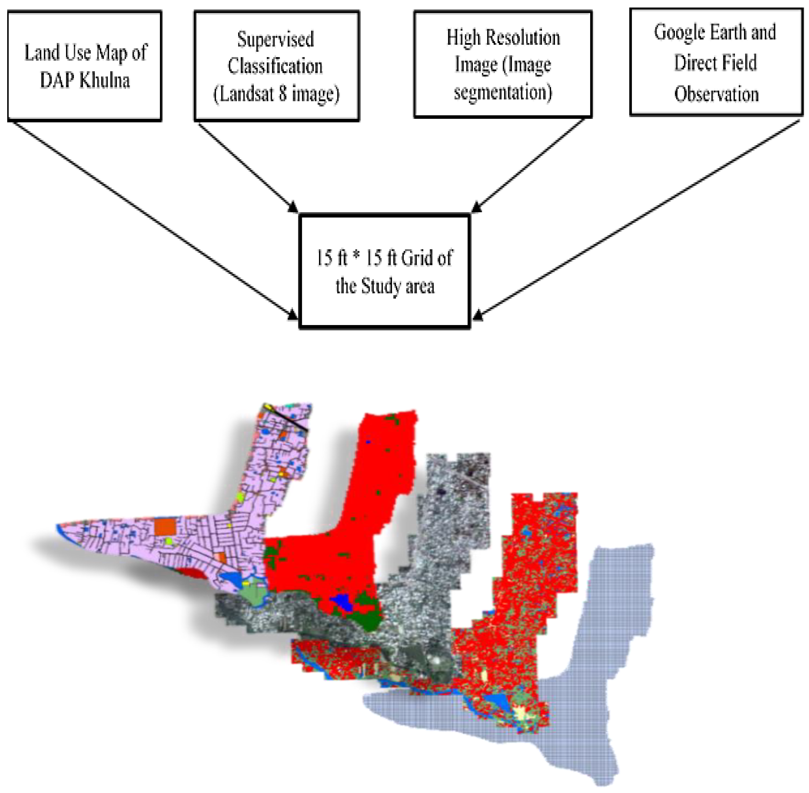
Figure 4.
Land-Cover Map of Ward 24.

Figure 5.
Electricity consumption footprint calculation and derivation. Source: a Household Survey of Ward 24 Residential Area (2015); [54]; b [55]; c [56]; d [57]; e [46].

Figure 6.
Natural gas consumption footprint calculation and derivation. Source: a Household Survey of Ward 24 Residential Area (2015), [54], b [55], c [56]; d [57]; e [46].

Figure 7.
Water consumption footprint calculation and derivation. Source: a Household Survey of Ward 24 Residential Area (RA) (2015); Khulna Water Supply and Sewerage Authority (WASA) (2015); b [58].
Figure 7.
Water consumption footprint calculation and derivation. Source: a Household Survey of Ward 24 Residential Area (RA) (2015); Khulna Water Supply and Sewerage Authority (WASA) (2015); b [58].

Figure 8.
Fuel consumption footprint calculation and derivation. Source: a Household Survey of Ward 24 Residential Area (RA) (2015); [59]; b [60].


Figure 10.
Waste generation rate footprint calculation and derivation. Source: a Waste Generation Rate (Survey 2015) for the population of 2015 of Ward 24 Residential Area. b [65].
Figure 10.
Waste generation rate footprint calculation and derivation. Source: a Waste Generation Rate (Survey 2015) for the population of 2015 of Ward 24 Residential Area. b [65].

Figure 11.
Food consumption footprint calculation and derivation. Source: 1 Household survey of Ward 24 RA (2015), [68]; 2 [66]).

Figure 12.
Goods consumption footprint calculation and derivation. Source: 1 Household survey of Ward 24 RA (2015); 2 GHG emissions; EIO-LCA (2015).
Figure 12.
Goods consumption footprint calculation and derivation. Source: 1 Household survey of Ward 24 RA (2015); 2 GHG emissions; EIO-LCA (2015).

Figure 13.
Services consumption footprint calculation and derivation. Source: 1 Household survey of Ward 24 RA (2015); 2 [66]).
Figure 13.
Services consumption footprint calculation and derivation. Source: 1 Household survey of Ward 24 RA (2015); 2 [66]).

Figure 14.
Global, National, and Local Perspectives of the Ecological Deficit.

Figure 15.
Per Capita Materials Consumption Percentage at the Household Level.

Figure 16.
Environmental Stress Visualization.


Table 1.
Considered components for the derivation of consumption footprint.
| Built-Up Footprint |
| Land–Residential; Land–Goods; Land–Services; Land–Transportation |
| Carbon Uptake Land Footprint |
|
Source [9].
Table 2.
Consumption footprint data requirements and data sources.
| Sl No. | Data Type | Data Sources |
|---|---|---|
| Objective 1: Household basis per-capita material consumption | ||
| 01. | Ward wise demographic data (2001, 2011) | Bangladesh Bureau of Statistics, Community Series |
| 02. | Consumption-related data (household level): food, water, goods, services, waste generation rate, trip generation, mode choice | Questionnaire survey |
| 03. | Unit price of electricity | West Zone Power Development Board |
| 04. | Gas cylinder characteristics and price | Basundhara LPG Gas Limited. |
| 05. | Current fuel price | Fuel Pump (direct interview) |
| 06. | Khulna city boundaries with road networks and facilities distribution | Khulna Development Authority (KDA) and Khulna City Corporation (KCC) |
| 07. | Khulna city available Transport Network | Urban and Regional Planning (URP), Khulna University of Engineering and Technology (KUET); Khulna Detailed Area Plan (DAP) by KDA |
| 08. | Khulna city water suppliers | KCC, KDA, Khulna Water Supply, and Sewerage Authority (KWASA) |
| 09. | Khulna city Master Plan | KDA |
| Objective 2: Ecological Stress Assessment and Visualization | ||
| 10. | Equivalency factors, yield factors, Sequestration factors | Berkeley Institute on the Environment (BIE), Stockholm Environment Institute (SEI), Intergovernmental Panel on Climate Change (IPCC), Global Footprint Network (GFN) |
| 11. | Landsat 8iImagery Red, green, and blue visible bands 30 m × 30 m resolution | United States Geological Survey (USGS) Website |
| 12. | QuickBird 0.61-m panchromatic imagery and high-resolution Google Earth imagery. | Department of URP, KUET, Google Inc |
Table 3.
Problems and advantages of different data types and image classifications.
| Data Type | Problems and Advantages a,b,c,d |
|---|---|
| Land-Use Map of DAP Khulna | The land-use map of DAP only identified the types of land use, but did not detect the microclasses within a specific land-use type, i.e., vegetation cover within the residential areas. |
| Landsat 8 (Supervised Classification) | Landsat images are suitable for larger study areas, while for smaller extents, a bias to any specific class is experienced. |
| High Resolution (Image Segmentation) | A high-resolution image with 0.6-m resolution is suitable for the image segmentation system. The segmented parts can be classified according to knowledge-based data, but it also identifies segments according to the pixel values or objects similarity, which generates some errors. |
| Ground Data (Knowledge-Based Classification) | Ground data-based classification or knowledge-based classification is treated as the most efficient land cover classification method as direct inputs by the user are incorporated into the system; however, for larger areas, this process is labor-intensive and time-consuming. |
Table 4.
Image classification accuracy assessment.
| Classification Methods | Overall Accuracy (%) | Kappa Coefficient |
|---|---|---|
| Supervised | 88.75 | 0.85 |
| Segmentation | 93.53 | 0.89 |
| Knowledge-Based | 93.67 | 0.91 |
Table 5.
Total footprint of ward 24 residential areas.
| Footprint Components | Footprint (Hectare) | Footprint (Global Hectare) | 1 Footprint (gha/capita) | |
|---|---|---|---|---|
| Carbon Footprint | Energy–Electricity | 2924.14 | 3684.416 | 0.1035 |
| Energy–Natural Gas | 2116.21 | 2666.42 | 0.0749 | |
| 2 Water | 11,197.223 | 14,108.501 | 0.000 | |
| Transportation–Fuel | 4604.37 | 5801.51 | 0.1629 | |
| Transportation–Asphalt | 173.44 | 218.53 | 0.0061 | |
| Waste | 759.33 | 956.75 | 0.0269 | |
| Food–Meat | 513.43 | 646.92 | 0.0182 | |
| Food–Fish | 320.65 | 404.02 | 0.0113 | |
| Food–Dairy | 350.85 | 442.07 | 0.0124 | |
| Food–Fruits and Vegetables | 432.54 | 544.99 | 0.0153 | |
| Food–Cereal | 520.17 | 655.41 | 0.0184 | |
| Food–Confectionary | 363.36 | 457.84 | 0.0129 | |
| Food–Drinks | 87.74 | 110.56 | 0.0031 | |
| Food–Others | 814.88 | 1026.74 | 0.0288 | |
| Goods–Furnishing and Equipment | 300.44 | 378.55 | 0.0106 | |
| Goods–Housekeeping | 140.154 | 176.594 | 0.0050 | |
| Goods–Others | 418.569 | 527.398 | 0.0148 | |
| Service–Education | 1537.34 | 1937.046 | 0.0544 | |
| Service–Health | 233.12 | 293.731 | 0.0082 | |
| Service–Entertainment | 442.33 | 557.338 | 0.0156 | |
| Service–Technical | 189.01 | 238.158 | 0.0067 | |
| Service–Administrative | 2787.31 | 3512.0087 | 0.0986 | |
| Built-up Land Footprint | Land–Residential | 105.87 | 265.74 | 0.0075 |
| Land–Goods | ||||
| Land–Services | ||||
| Land–Transportation | ||||
| Total Footprint | 20,135.253 | 25,502.74 | 0.7161 | |
Note: 1 Projected population of 2015 (using the population data of 1991, 2001, and 2011 from the Bangladesh Bureau of Statistics, or BBS) of the Ward 24 Nirala residential area is 35613; 2 Water footprint of the area is omitted from the calculation.
Table 6.
Biocapacity calculation (Ward 24).
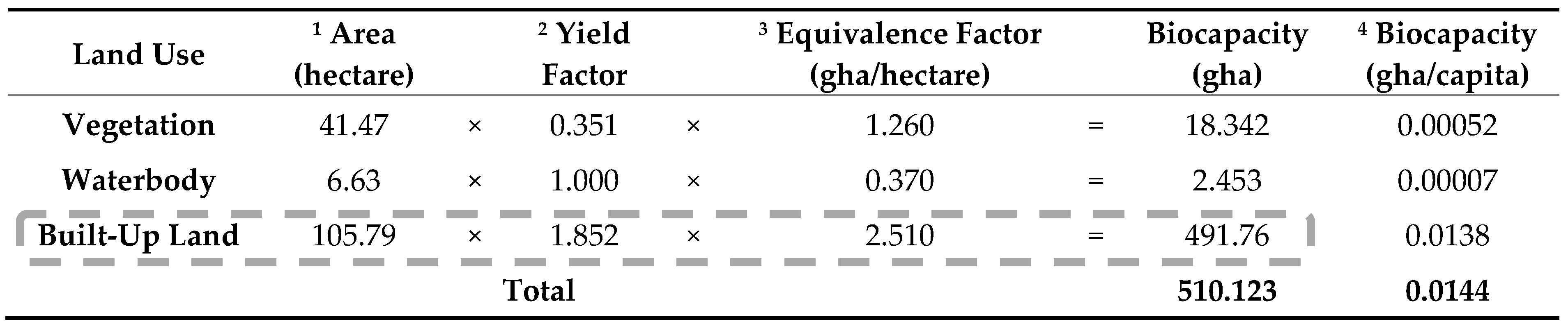
Table 7.
Stress area delineation.

© 2018 by the authors. Licensee MDPI, Basel, Switzerland. This article is an open access article distributed under the terms and conditions of the Creative Commons Attribution (CC BY) license (http://creativecommons.org/licenses/by/4.0/).
Share and Cite
MDPI and ACS Style
Khan, M.S.; Uddin, M.S. Household Level Consumption and Ecological Stress in an Urban Area. Urban Sci. 2018, 2, 56. https://doi.org/10.3390/urbansci2030056
AMA Style
Khan MS, Uddin MS. Household Level Consumption and Ecological Stress in an Urban Area. Urban Science. 2018; 2(3):56. https://doi.org/10.3390/urbansci2030056
Chicago/Turabian StyleKhan, Md. Shakil, and Muhammad Salaha Uddin. 2018. "Household Level Consumption and Ecological Stress in an Urban Area" Urban Science 2, no. 3: 56. https://doi.org/10.3390/urbansci2030056