Comparison Study of the k − k_L − ω and γ − Re_θ Transition Model in the Open-Water Performance Prediction of a Rim-Driven Thruster

Abstract

The present work examines the capabilities of two transition models implemented in ANSYS Fluent in the open-water performance prediction of a rim-driven thruster (RDT). The adopted models are the three-equation $k-k_L-\omega$ and the four-equation $\gamma -R{e}_{\theta }$ models. Both of them are firstly tested on a ducted propeller. The numerical results are compared with available experimental data, and a good correlation is found for both models. The simulations employing two transition models are then carried out on a four-bladed rim-driven thruster model and the results are compared with the SST $k-\omega$ turbulence model. It is observed that the streamline patterns on the blade surface are significantly different between the transition and fully turbulent models. The transition models can reveal the laminar region on the blade while the fully turbulent model assumes the boundary layer is entirely turbulent, resulting in a considerable difference in torque prediction. It is noted that unlike the fully turbulent model, the transition models are quite sensitive to the free-stream turbulence quantities such as turbulent intensity and turbulent viscosity ratio, as these quantities determine the onset of the transition process. The open-water performance of the studied RDT and resolved flow field are also presented and discussed.

1. Introduction

Computational fluid dynamics (CFD) has become a very powerful tool in analyzing engineering problems in recent decades, such as the performance prediction of marine propellers. The widest application is achieved by solving the Reynolds averaged Navier–Stokes (RANS) equations because compared with other approaches, such as direct numerical simulation (DNS) or large eddy simulation (LES), the RANS method is much cheaper with reasonable accuracy. To solve the Reynolds stress terms in the RANS equations, turbulence models based on the Boussinesq hypothesis are introduced to simplify this problem. Among them the most popular ones are the $k-ϵ$ and $k-\omega$ series models. Since these turbulence models are built on the assumption that the resolved flow field is fully turbulent, they are incapable of predicting the transition phenomenon which is frequently encountered in physical problems. In order to improve the potential of the currently existing turbulence models for resolving transitional flows, a lot of efforts have been made to develop models which can predict the transition process from laminar to turbulent flows. There are generally two ways of achieving this: one is to couple the transition correlations, which are obtained from available experimental data, into the turbulence models; the other is to solve additional transport equations to account for the transitional effects. However, even if a transition model is successfully developed, it is still questionable whether it can be implemented into modern CFD codes which are usually based on unstructured grids and parallel execution, as most transition models are still using nonlocal variables or integral terms. Single-point models which use only local variables are required for a general application. In ANSYS Fluent, there are two transition models available, i.e., the three-equation $k-k_L-\omega$ and four-equation $\gamma -R{e}_{\theta }$ models. Both models introduce additional transport equations to include the transitional effects in flows. The present work aims to test the capabilities of these two transition models in the prediction of the hydrodynamic characteristics of a rim-driven thruster. As it has been confirmed in the research of Kuiper [1], on the propeller of model scale, there is often a large area of laminar flow on both sides of the blade surface. In order to investigate the potential reason for the discrepancy between simulations and experiments, especially at high loading conditions, Wang and Walters [2] employed the Loci/CHEM flow solver to study the marine propeller 5168 using the $k-k_L-\omega$ transition model. The SST $k-\omega$ turbulence model was also used for comparison. The simulation results were analyzed and compared with experimental data. It was found that the transition model showed better performance in resolving the flow field and therefore improved the prediction accuracy, while the standard SST $k-\omega$ model indicated an excessive dissipation of vortex cores. Pawar and Brizzolara [3] investigated the propeller of an autonomous underwater vehicle (AUV) which often operates at low Reynolds number in the laminar-to-turbulent transition region. The global and local hydrodynamic characteristics of open and ducted propellers were investigated with the $\gamma -R{e}_{\theta }$ transition model. The results demonstrated that the transition model was able to predict complex flow physics such as leading-edge separation, tip leakage vortex, and the separation bubble on the outer surface of the duct.

Baltazar et al. [4] examined the open-water performance of a conventional marine propeller under different Reynolds numbers using the SST $k-\omega$ turbulence model and the $\gamma -R{e}_{\theta }$ transition model. They found that the inlet quantities had different influences on the two models, with the $\gamma -R{e}_{\theta }$ transition model being highly dependent on flow quantities while the SST $k-\omega$ turbulence model was hardly affected. Therefore, the correct information on the turbulence intensity and eddy viscosity was necessary to improve the prediction accuracy. In the $\gamma -R{e}_{\theta }$ transition model proposed by Menter et al. [5], two important parameters in the transport equation of the intermittency $\gamma$ were kept proprietary, namely, $F_{length}$ and $F_{onset}$, which controlled the length of the transition region and the onset location of the transition, respectively. In order to tackle this issue, Suluksna et al. 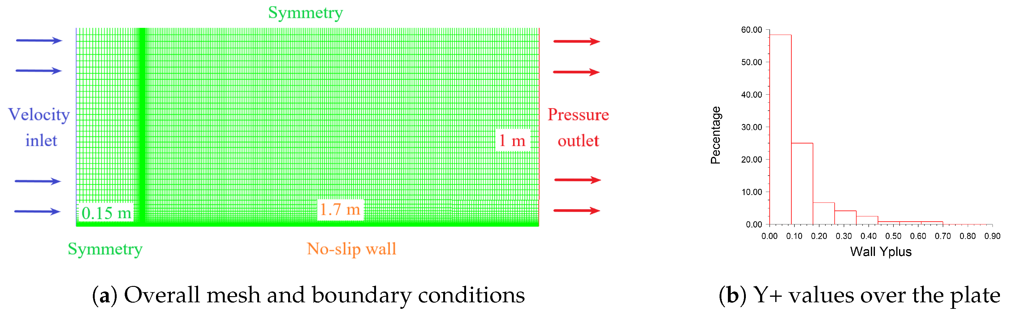[6] proposed some mathematical expressions for these specific parameters to close the model, which were assumed to be valid for both natural and bypass transition in boundary layers with and without pressure gradient. Afterwards, several test cases were carried out on a transitional flow over a flat plate and the results were compared with experimental data. Generally, the model with the proposed parameters showed a reasonable agreement with the experiment.

The RDT resembles a ducted propeller in structural design as both contain a propeller and a duct. But unlike a ducted propeller, there is no tip clearance for the RDT propeller. Instead, a gap channel is formed by the rim and duct surfaces. The scheme of an RDT layout is presented in Figure 1 [7]. Depending on whether there is a central hub or not, the RDT can be roughly classified into a hub type and a hubless type, as shown in Figure 2. Both types have their own advantages and disadvantages [8]. For example, the hub-type RDT has a greater structural strength, and bearings can be installed in the hub to reduce friction. While the hubless type has a simpler structure and a higher hydrodynamic efficiency. Due to the appealing potential the RDT system possesses, many research studies have been conducted on the modeling and evaluation of RDTs. Dubas et al. [9] employed the OpenFOAM solver for the study of rotor–stator interaction. Song et al. [10] compared the open-water performance between the hub and hubless type of RDTs using numerical simulations. Cai et al. [11] numerically analyzed the performance of an RDT and considered the effect of the rim length. Gaggero [12] adopted a RANS method to optimize the propeller blade in an RDT in order to improve its hydrodynamic efficiency and cavitation performance. Liu and Vanierschot [7] and Liu et al. [13] compared the hydrodynamic performance of an RDT and a ducted propeller with the same configuration at a model scale and investigated the transitional flow on the propeller blades. The influence of the gap flow on the propeller performance was investigated by Cao et al. [14].

For the model-scale RDT, the flow on the propeller often tends to be in a laminar or transitional regime. Therefore, transitional modeling is required to better resolve the boundary layer in order to achieve an improved hydrodynamic performance prediction. The structure of this paper is organized in this way: firstly, a brief description of the transition models used in this study is presented; then, some validation studies are carried out to test the capabilities of the transition models, followed by the results and discussion on RDT simulations.

2. Numerical Modeling

The Reynolds averaged Navier–Stokes (RANS) equations for incompressible Newtonian fluids are given by

$$\frac{\partial u_i}{\partial x_i}=0,$$

(1)

$$\begin{array}{c}\hfill \rho \left(\frac{\partial u_i}{\partial t}+u_j\frac{\partial u_i}{\partial x_j}\right)=-\frac{\partial p}{\partial x_i}+\frac{\partial }{\partial x_j}\left[\mu \left(\frac{\partial u_i}{\partial x_j}+\frac{\partial u_j}{\partial x_i}\right)\right]+\\ \hfill \frac{\partial }{\partial x_j}\left(-\rho \overline{u_i^{\prime }{u}_j^{\prime }}\right),\end{array}$$

where $\rho$ is the fluid density, $u_i(i,j=1,2,3)$ is the turbulence averaged velocity component, t is the flow time, p is the pressure, $\mu$ is the dynamic viscosity, and $-\rho \overline{u_i^{\prime }{u}_j^{\prime }}$ is the Reynolds stress term. Based on the Boussinesq hypothesis, for incompressible fluids, the Reynolds stress can be related to the mean strain rate $S_{ij}=\frac{1}{2}\left(\frac{\partial u_i}{\partial x_j}+\frac{\partial u_j}{\partial x_i}\right)$ and eddy viscosity as follows

$$-\rho \overline{u_i^{\prime }{u}_j^{\prime }}=2{\mu }_t{S}_{ij}-\frac{2}{3}\rho k{\delta }_{ij},$$

(2)

where ${\mu }_t$ is the turbulent viscosity and ${\delta }_{ij}$ is the Kronecker symbol.

The formulation of closure to the above equations is called turbulence modeling. Currently the most popular turbulence models in industrial applications are the two-equation ones, like the earliest $k-ϵ$ model. This model has gone through many modifications to improve and extend its applicability. It has great capabilities for free-shear flows but behaves poorly in flows with adverse pressure gradient. To tackle this issue, the $k-\omega$ model by was proposed, which has better performance for flows with weak adverse pressure gradient. Again, several updates have been made to this model to enhance its performance.

2.1. SST $k-\omega$ Model

The SST $k-\omega$ turbulence model developed by Menter [15] is an improved version of the original $k-\omega$ model. It has robust near wall treatment and the ability to compute flows with moderate adverse pressure gradients by combining the $k-ϵ$ model and the $k-\omega$ model with blending functions. The transport equations for the turbulent kinetic energy k and the specific turbulent dissipation rate $\omega$ are given as

$$\rho \left(\frac{\partial k}{\partial t}+u_j\frac{\partial k}{\partial x_j}\right)=\widetilde{P_k}+\frac{\partial }{\partial x_j}\left[\left(\mu +{\mu }_t{\sigma }_k\right)\frac{\partial k}{\partial x_j}\right]-{\beta }^{*}\rho k\omega ,$$

(3)

$$\begin{array}{c}\hfill \rho \left(\frac{\partial \omega }{\partial t}+u_j\frac{\partial \omega }{\partial x_j}\right)=C_{\alpha }\rho S^2+\frac{\partial }{\partial x_j}\left[\left(\mu +{\mu }_t{\sigma }_{\omega }\right)\frac{\partial \omega }{\partial x_j}\right]-C_{\beta }\rho {\omega }^2\\ \hfill +2(1-F_1){\sigma }_{\omega 2}\frac{\rho }{\omega }\frac{\partial k}{\partial x_j}\frac{\partial \omega }{\partial x_j}.\end{array}$$

(4)

The turbulent eddy viscosity is calculated as

$${\mu }_t=\frac{\rho a_{1}k}{max(a_1\omega ,S{F}_2)},$$

(5)

where $a_1$ is a model constant, S is the modulus of the mean strain rate $S_{ij}$ as defined above, and $F_2$ is the blending function defined as

$$F_2=tanh\left[{\left[max\left(\frac{2\sqrt{k}}{{\beta }^{*}\omega y},\frac{500\mu }{y^2\omega }\right)\right]}^2\right],$$

(6)

where ${\beta }^{*}$ is a model constant and y is the distance to the nearest wall. Detailed information about the definition of functions and values of model constants can be found in [15].

2.2. $\gamma -R{e}_{\theta }$ Transition Model

The $\gamma -R{e}_{\theta }$ transition model is a correlation-based transition model using local variables, which contains two additional transport equations, i.e., for the intermittency $\gamma$ and the transition onset’s momentum thickness Reynolds number ${\widetilde{Re}}_{\theta t}$. The additional transport equations are not used to model the transition physics but to provide a framework within which empirical correlations can be made for specific cases. The first quantity, intermittency, is a measure of whether the flow is laminar or turbulent. $\gamma =0$ means a continuous laminar flow, and $\gamma =1$ means a continuous turbulent flow. Therefore, the intermittency equation is used to trigger the local transition process. The second quantity is the transition onset’s Reynolds number $R{e}_{\theta t}$, which is used to account for the nonlocal influence of the turbulence intensity on the boundary layer, as well as to relate the empirical correlation to the onset criteria in the intermittency equation. Finally, the intermittency function is coupled with the original SST $k-\omega$ model, which is used to turn on the production term of the turbulent kinetic energy downstream of the transition location and the equation for the ${\widetilde{Re}}_{\theta t}$ can pass the information on the free-stream conditions into the boundary layer. The formulated equations for the intermittency $\gamma$ and transition’s momentum thickness Reynolds number ${\widetilde{Re}}_{\theta t}$ are given by:

$$\rho \left(\frac{\partial \gamma }{\partial t}+\frac{\partial \left(u_j\gamma \right)}{\partial x_i}\right)=P_{\gamma }-E_{\gamma }+\frac{\partial }{\partial x_i}\left[\left(\mu +\frac{{\mu }_t}{{\sigma }_f}\right)\frac{\partial \gamma }{\partial x_j}\right],$$

(7)

$$\rho \left(\frac{\partial {\widetilde{Re}}_{\theta t}}{\partial t}+\frac{\partial u_j{\widetilde{Re}}_{\theta t}}{\partial x_j}\right)=P_{\theta t}+\frac{\partial }{\partial x_j}\left[{\sigma }_{\theta t}\left(\mu +{\mu }_t\right)\frac{\partial {\widetilde{Re}}_{\theta t}}{\partial x_j}\right],$$

(8)

where $P_{\gamma }$ and $E_{\gamma }$ are the source terms which control the production and destruction of the intermittency, ${\sigma }_f$ is the model constant and is equal to 1, $P_{\theta t}$ is the production term that is designed to relate the transported scalar ${\widetilde{Re}}_{\theta t}$ to the local empirical $R{e}_{\theta t}$ outside the boundary layer, and ${\sigma }_{\theta t}$ is the model constant and is equal to 10. The detailed definitions of the above terms can be found in Menter et al. [5].

By solving the above two equations, an effective intermittency ${\gamma }_{eff}$ is obtained. It is then incorporated into the transport equations for k and $\omega$ in the SST $k-\omega$ model:

$$\rho \left(\frac{\partial k}{\partial t}+\frac{\partial \left(u_{j}k\right)}{\partial x_i}\right)={\gamma }_{eff}(P_k-D_k)+\frac{\partial }{\partial x_i}\left[\left(\mu +{\sigma }_k{\mu }_t\right)\frac{\partial k}{\partial x_j}\right],$$

(9)

$$\rho \left(\frac{\partial \omega }{\partial t}+\frac{\partial \left(u_j\omega \right)}{\partial x_i}\right)=\alpha \frac{P_k}{{\nu }_t}-D_{\omega }+C{d}_{\omega }+\frac{\partial }{\partial x_i}\left[\left(\mu +{\sigma }_k{\mu }_t\right)\frac{\partial \omega }{\partial x_j}\right].$$

(10)

2.3. $k-k_L-\omega$ Model

Unlike the $\gamma -R{e}_{\theta }$ model, the $k-k_L-\omega$ model is a physics-based model. Three additional transport equations are solved to account for the effects of pretransition fluctuations, including the bypass and natural transitions. In this model, the concept of laminar kinetic energy $k_L$ is employed, which represents the velocity fluctuations in the pretransitional regions. With the increase in turbulence intensity in the free stream, the mean velocity profiles in these regions are distorted, and more intensive streamwise fluctuations can take place, which finally break down and result in the transition process. This happens when the characteristic timescale for the turbulence production is smaller than the viscous diffusion timescale of the pretransitional fluctuations. It is assumed that the production of $k_L$ is a result of the interaction between the Reynolds stresses and the mean shear. The total energy of $k_L$ and $k_T$ is constant, which means that when the transition occurs, the energy is transferred from $k_L$ to $k_T$, i.e., a redistribution of energy. The three additional transport equations for $k_T$, $k_L$, and $\omega$ are given by:

$$\begin{array}{c}\hfill \rho \left(\frac{\partial k_T}{\partial t}+\frac{\partial \left(u_j{k}_T\right)}{\partial x_i}\right)=P_{k_T}+R_{BP}+R_{NAT}-\rho \omega k_T-D_{k_T}\\ \hfill +\frac{\partial }{\partial x_j}\left[\left(\mu +\frac{{\alpha }_T}{{\sigma }_k}\right)\frac{\partial k_T}{\partial x_j}\right],\end{array}$$

(11)

$$\rho \left(\frac{\partial k_L}{\partial t}+\frac{\partial \left(u_j{k}_L\right)}{\partial x_i}\right)=P_{k_L}-R_{BP}-R_{NAT}-D_L+\frac{\partial }{\partial x_j}\left[\mu \frac{\partial k_L}{\partial x_j}\right],$$

(12)

$$\begin{array}{c}\hfill \rho \left(\frac{\partial \omega }{\partial t}+\frac{\partial \left(u_j\omega \right)}{\partial x_i}\right)=C_{\omega 1}\rho \frac{\omega }{k_T}{P}_{k_T}+\left(\frac{C_{\omega R}}{f_W}-1\right)\rho \frac{\omega }{k_T}(R_{BP}+R_{NAT})\\ \hfill -C_{\omega 2}\rho {\omega }^2+C_{\omega 3}\rho f_{\omega }{\alpha }_T{f}_W^2\frac{\sqrt{k_T}}{d^3}+\frac{\partial }{\partial x_j}\left[\left(\mu +\frac{{\alpha }_T}{{\sigma }_{\omega }}\right)\frac{\omega }{x_j}\right].\end{array}$$

(13)

The various terms in the model equations represent production, destruction, and transport mechanisms, where $P_{k_T}$, $D_{k_T}$ are, respectively, the production and destruction of turbulent kinetic energy, $R_{BP}$ and $R_{NAT}$ represent the effect of bypass and natural transitions, $C_{\omega }$s and ${\sigma }_{\omega }$ are model constants, $f_{\omega }$ and $f_W$ are the damping functions, and ${\alpha }_T$ is the effective diffusivity. Detailed definitions of the above terms can be found in Walters and Cokljat [16].

The SIMPLE (Semi-Implicit Method for Pressure Linked Equations) algorithm is adopted for the pressure and velocity coupling. Second-order upwind schemes are used for the discretization of momentum and turbulence terms. Moreover, the moving reference frame (MRF) approach is employed to handle the rotation of the propeller. The MRF method is a steady-state approximation for the analysis of situations involving domains that are rotating relatively to each other. Previous work showed that it gave similar results compared to the sliding-mesh method, which is computationally much more expensive [17]. The governing equations for the flow in the selected rotating zone are solved in a relative rotating frame. Namely, the computational domain is divided into two subdomains, one which contains the rotating propeller and the other one which is fixed.

The hydrodynamic coefficients are defined as:

$$J=\frac{v_a}{nD},$$

(14)

$$K_T=\frac{T}{\rho n^2{D}^4},$$

(15)

$$K_Q=\frac{Q}{\rho n^2{D}^5},$$

(16)

$$\eta =\frac{J}{2\mathsf{\pi }}\frac{K_T}{K_Q},$$

(17)

$$C_p=\frac{p-p_{\infty }}{\frac{1}{2}\rho v^2},$$

(18)

$$C_f=\frac{{\tau }_w}{\frac{1}{2}\rho v^2},$$

(19)

where $V_a$ is the inflow velocity, n is the rotational rate of the propeller, D is the diameter of the propeller, and J, $K_t$, T, $K_q$, Q and $\eta$ are, respectively, the advance coefficient, the total thrust coefficient, the total thrust, the total torque coefficient, the total torque, and the efficiency. $C_p$ is the pressure coefficient, p is the local pressure, $p_{\infty }$ is the free-stream pressure, v is the effective velocity of the propeller, which is equal to $\sqrt{V_a^2+{\left(0.7\pi nD\right)}^2}$, and ${\tau }_w=\mu \frac{\partial u}{\partial y}{|}_{y=0}$ (u is the flow velocity along the blade surface, y is the normal distance).

Based on the grid study in Liu et al. [13] for the SST $k-\omega$ model, in this work, the meshes used for the uncertainty evaluation included a medium mesh with a total cell number of about 18 M (million) and a fine mesh of about 25 M. To avoid the influence of a near-wall treatment due to the mesh resolution in the boundary layer, the prism mesh in both cases were kept the same. The results between different meshes for the $\gamma -R{e}_{\theta }$ transition model are compared in

Table 1. Grid discretization error estimation for the $\gamma -R{e}_{\theta }$ transition model.

Advance Coefficient	Hydrodynamic Coefficient	Medium Mesh	Fine Mesh	Grid Uncertainty (%)
$J=0.1$	$K_{\mathrm{tp}}$	0.262	0.259	−1.15
	$K_{\mathrm{tn}}$	0.137	0.140	2.19
	$K_{\mathrm{tr}}$	0.074	0.072	2.70
	10 $K_{\mathrm{qp}}$	0.434	0.429	−1.15
	10 $K_{\mathrm{qr}}$	0.171	0.173	1.17

. It can be seen that the grid uncertainty was of the same order as the one of the SST $k-\omega$ model and was therefore acceptable [13]. Therefore, the medium mesh was considered to be sufficient to resolve the flow field and was adopted in subsequent simulations.

3. Results and Discussion

3.1. Test Cases

3.1.1. Flow over a Flat Plate

To test the capabilities of the $\gamma -R{e}_{\theta }$ and $k-k_L-\omega$ transition models, a benchmark test case was examined, namely, the flow over a flat plate without a pressure gradient. The computational domain and boundaries conditions are shown in Figure 3. The flat plate had a length of 1.7 m. It was placed 0.15 m downstream from the inlet, as indicated by the black circle. A symmetry boundary condition was used to guide the uniform flow from the inlet to the plate. A pressure outlet was adopted at the end of the plate and a no-slip boundary condition was used for the plate.

The transition onset is generally based on the disturbance strength in the boundary layer, which is determined by the flow properties of the free stream, like the turbulence intensity ($TI$). When the flow develops, there will be a decay in $TI$, and the turbulent viscosity ratio ($TVR$) reflects the decay speed. Therefore, different combinations of turbulence intensities, with the turbulent viscosity ratio taken from the experiments, were assessed, and the results are given in Figure 4. $R{e}_x$ is the Reynolds number determined by the position on the plate along the flow direction, and $C_f$ is the skin friction coefficient. In this figure, the gray and blue lines represent the analytical solutions for laminar and turbulent flows, respectively. From the results, it is observed that the values for the turbulent intensity can influence the location of the transition onset, because a higher turbulent viscosity ratio will reduce the decay of the turbulent intensity, resulting in an earlier onset of the transition process. Therefore, to accurately evaluate a solution for a practical problem, an appropriate assessment of these values at the inlet is very important. Generally, the transition model can robustly reflect the flow physics.

3.1.2. Open-Water Performance of a Ducted Propeller

Another test case was conducted for a ducted propeller, for which open-water tests were available. A hybrid meshing strategy was employed for the mesh generation, as shown in Figure 5. A grid independence study was carried out first to ensure a numerical accuracy compared to previous work [13], in which a two-grid assessment procedure was conducted and the grid uncertainty was proved to be less than 2%. The Reynolds number was $6.42\times {10}^5$, if determined by the velocity and chord length of the propeller at 0.7R. The design point, where the peak efficiency was achieved, was defined as $J=0.6$ in this case.

Figure 6 provides a comparison between the two transition models and experimental measurements obtained from Oosterveld [18]. A good correlation was found between both transition models and experimental data. It was noted that the propeller and duct thrust predicted by the $\gamma -R{e}_{\theta }$ transition model was quite close to those predicted by the SST $k-\omega$ turbulence model. A major difference was found for the propeller torque prediction, where the SST $k-\omega$ model obviously gave higher values for the propeller torque under all advance coefficients.

To find out the reasons, the components of the thrust and torque were compared, as provided in

Table 2. Contribution of pressure and shear component to the thrust coefficient (Kt) and torque coefficient (Kq) of the RDT at $J=0.1$.

$\mathit{J}=0.1$	SST $\mathit{k}-\mathit{\omega }$ Model		$\mathit{\gamma }-{\mathit{Re}}_{\mathit{\theta }\mathit{t}}$ Model		$\mathit{k}-{\mathit{k}}_{\mathit{L}}-\mathit{\omega }$ Model
	Kt	10 Kq	Kt	10 Kq	Kt	10 Kq
Pressure	0.239	0.378	0.234	0.372	0.217	0.348
Shear	−0.005	0.042	−0.004	0.028	−0.004	0.028
Total	0.234	0.42	0.238	0.399	0.213	0.376

and

Table 3. Contribution of pressure and shear component to the thrust coefficient (Kt) and torque coefficient (Kq) of the RDT at $J=0.5$.

$\mathit{J}=0.5$	SST $\mathit{k}-\mathit{\omega }$ Model		$\mathit{\gamma }-{\mathit{Re}}_{\mathit{\theta }\mathit{t}}$ Model		$\mathit{k}-{\mathit{k}}_{\mathit{L}}-\mathit{\omega }$ Model
	Kt	10 Kq	Kt	10 Kq	Kt	10 Kq
Pressure	0.160	0.264	0.157	0.263	0.135	0.232
Shear	−0.006	0.047	−0.004	0.026	−0.004	0.026
Total	0.154	0.311	0.153	0.289	0.131	0.258

, which present the results from the SST $k-\omega$, the $\gamma -R{e}_{\theta }$, and the $k-k_L-\omega$ models. It can be observed that the pressure was the dominating factor both in thrust and torque and that the difference in torque prediction between the two models was mainly caused by the shear stress. As the transition models gave lower values for the skin friction, a slightly higher thrust and a lower torque were expected.

3.2. Results and Discussion on the RDT

In this section, the simulation results using the fully turbulent and transition models are presented and analyzed. To better understand the transition process, different propeller speeds were considered as the Reynolds number needs to be high enough to trigger the transitional effects in the model. The revolution rate of 10 rps and 20 rps were examined, and the Reynolds number at the propeller section of $r/R=0.7$ was $5.07\times {10}^5$ and $1.14\times {10}^6$, respectively.

3.2.1. Flow Patterns on the Propeller

The distribution of the skin friction coefficient $C_f$ on both pressure and suction sides of the propeller blade with constrained streamlines by all three models is provided in Figure 7. The pattern of the streamline is an indication of the flow regime over the blade. As the direction of the streamline is a result of friction and centrifugal forces, the streamline is always deflected to the dominant force. When the flow is turbulent, the friction force has a greater influence compared to the centrifugal force; therefore, the streamline is forced to go along the tangential direction over the blade. However, in the case of a laminar flow, the opposite phenomenon can be observed, and the streamline is outwardly oriented. It is also observed that the flows predicted by the transition models are more complex than those by the turbulence model, which is probably caused by the transitional flows on the hub before the blade.

The difference in streamline patterns can be clearly observed between the fully turbulent and transition models. Moreover, the skin friction is obviously larger in the turbulent flow than in the laminar flow, because a greater wall shear stress is achieved in a turbulent boundary layer, where the velocity gradient at the wall is steeper. The skin friction distributions on the blade surface predicted by the two transition models are quite close, except for the difference found at the blade tip. The $k-k_L-\omega$ model gives higher values for $C_f$, and there is obviously a change in the direction of the streamlines, indicating the flow is changing from a laminar regime to a turbulent one. Figure 8 provides a comparison of the kinetic energy distribution near the blade by the two transition models. There is clearly more turbulent kinetic energy (TKE) production at the blade tip region in the $k-k_L-\omega$ model, resulting in a change in flow regime. In

Table 4. Contribution of pressure and shear component to the thrust coefficient (Kt) and torque coefficient (Kq) of the propeller at $J=0.5$.

	$\mathit{k}-{\mathit{k}}_{\mathit{L}}-\mathit{\omega }$ Model		$\mathit{\gamma }-{\mathit{Re}}_{\mathit{\theta }\mathit{t}}$ Model
	Pressure	Shear	Pressure	Shear
Ktp	0.133	−0.003	0.155	−0.003
Ktd	0.007	−0.002	0.004	−0.002
Ktr	0.029	−0.003	0.034	−0.001
10 Kqp	0.228	0.015	0.261	0.02
10 Kqr	0	0.165	0	0.153

, the thrust and torque of different components predicted by both models are compared. The $\gamma -R{e}_{\theta }$ model gives higher values for propeller thrust and torque in both pressure and shear forces. However, since there are currently no experimental data available for the RDT, it is hard to conclude which model has a higher accuracy in performance prediction.

3.2.2. Influence of the Reynolds Number

As discussed above, the fully turbulent model assumes that the boundary layer on the blade is always fully turbulent, despite the fact that there might be transitional flows locally. By comparison, the transition models have the potential to capture this phenomenon. However, it has also been observed in previous work that the streamlines are almost all directed outwardly, i.e., the flow is in a laminar regime over the entire blade surface. This also explains the negligible difference in performance prediction when changing the $TI$ and $TVR$ values at the inlet. As the Reynolds number is below the critical value, the transitional effects are not yet activated. Therefore, to further investigate how the onset of the transition is related to the turbulent intensity, a higher rotational propeller rotational rate was considered.

The influence of the turbulence intensity of the free stream on the transition process on the blade surface is presented in Figure 9. Three combinations of $TI$ and $TVR$ values were investigated. The $TI$ at the inlet was set constant, therefore the fluctuations close to the thruster were based on the $TVR$. The higher values of $TVR$ reduced the decay of $TI$, resulting in an earlier onset of the transition. It was clearly observed that with the increase in $TVR$, the turbulent effect became more pronounced at the blade tip, which was indicated by a larger skin friction. It was also noted that the $k-k_L-\omega$ model was not as sensitive to these inlet parameters as the $\gamma -R{e}_{\theta }$ model, and the skin friction distribution and streamline pattern were very close under different disturbances.

In order to figure out the reasons behind the difference in propeller performance prediction between the the $k-k_L-\omega$ and the $\gamma -R{e}_{\theta }$ models, the pressure and skin friction coefficients over the blade surfaces predicted by both transition models are presented in Figure 10, Figure 11, Figure 12 and Figure 13. In general, the pressure and skin friction distribution over the blade surfaces between the two transition models are quite similar. The pressure gradually becomes lower near the center of the blade suction side, and there is a small area of transition at the trailing edge close to the blade root. On the pressure side, flow separation is observed at the leading edge, which causes a sudden change in pressure distribution. The pressure difference between the blade pressure and suction sides for the $\gamma -R{e}_{\theta }$ model is generally larger than that of the $k-k_L-\omega$ model, which explains the larger propeller thrust production from the pressure component. As for the skin friction coefficient, the discrepancy between the two models can be neglected.

4. Conclusions

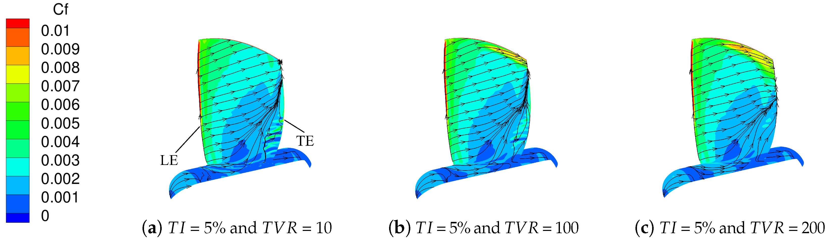
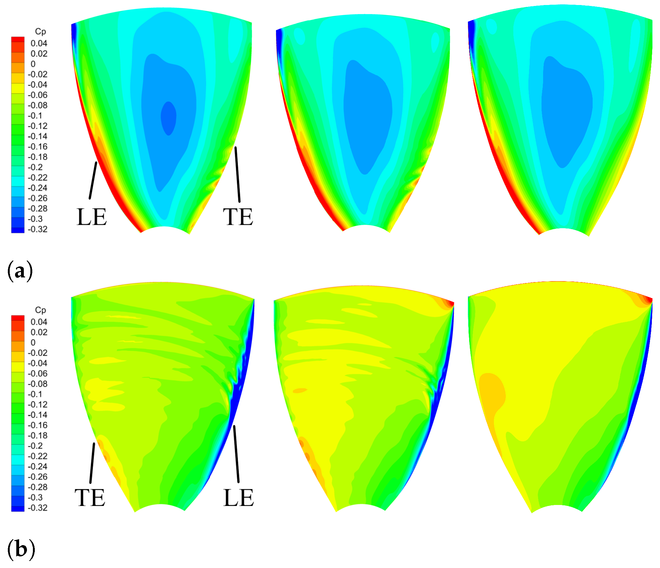
Laminar-to-turbulent transition flows are often observed on marine propellers at model scales. Accurately resolving this flow phenomenon can significantly improve the performance prediction of the propeller. In this work, the capabilities of the $k-k_L-\omega$ and $\gamma -R{e}_{\theta }$ transition models implemented in ANSYS Fluent’s flow solver were tested for the performance prediction of a rim-driven thruster. Different test cases were firstly considered to ensure the quality of the numerical simulations. From the validation study using a ducted propeller, it was concluded that the transition models exhibited better performance than a fullt turbulent model. The predicted thrusts of the propeller and duct, which were mainly based on the pressure contribution, were quite close using different models. However, the propeller torque was exceptional. When there were transitional flows, the transition models gave lower values for the torque due to the smaller shear stress prediction. This was a result of the laminar boundary layer, and the streamlines in that situation were more outwardly oriented due to the centrifugal acceleration. A comparison between the $k-k_L-\omega$ and $\gamma -R{e}_{\theta }$ transition models in the hydrodynamic performance prediction of an RDT was then conducted. From the results, it was found that there was a small difference between the two models. The $k-k_L-\omega$ predicted more local turbulent regions such as at the blade tip, and therefore, the skin friction was higher in that region than that of the $\gamma -R{e}_{\theta }$ model. The $\gamma -R{e}_{\theta }$ model predicted a higher propeller thrust, especially for the pressure component, but it is at present not certain which model is more accurate. More research is required for verification.

References

1. Kuiper, G. Cavitation Inception on Ship Model Propeller. Ph.D. Thesis, Delft University of Technology, Delft, The Netherlands, 1981. [Google Scholar]
2. Wang, X.; Walters, K. Computational Analysis of Marine-Propeller Performance Using Transition-Sensitive Turbulence Modeling. J. Fluids Eng. 2012, 134, 071107. [Google Scholar] [CrossRef]
3. Pawar, S.; Brizzolara, S. Relevance of Transition Turbulent Model for Hydrodynamic Characteristics of Low Reynolds Number Propeller. Appl. Ocean Res. 2019, 87, 165–178. [Google Scholar] [CrossRef]
4. Baltazar, J.; Rijpkema, D.; de Campos, J.F. On the use of the γ R e ˜ θ t transition model for the prediction of the propeller performance at model-scale. Ocean Eng. 2018, 170, 6–19. [Google Scholar] [CrossRef]
5. Menter, F.R.; Langtry, R.B.; Likki, S.R.; Suzen, Y.B.; Huang, P.G.; Völker, S. A Correlation-Based Transition Model Using Local Variables—Part I: Model Formulation. J. Turbomach. 2006, 128, 413–422. [Google Scholar] [CrossRef]
6. Suluksna, K.; Dechaumphai, P.; Juntasaro, E. Correlations for modeling transitional boundary layers under influences of freestream turbulence and pressure gradient. Int. J. Heat Fluid Flow 2009, 30, 66–75. [Google Scholar] [CrossRef]
7. Liu, B.; Vanierschot, M. Numerical Study of the Hydrodynamic Characteristics Comparison between a Ducted Propeller and a Rim-Driven Thruster. Appl. Sci. 2021, 11, 4919. [Google Scholar] [CrossRef]
8. Yan, X.P.; Liang, X.X.; Wu, O.Y.; Liu, Z.L.; Liu, B.; Lan, J.F. A Review of Progress and Applications of Ship Shaft-less Rim-Driven Thrusters. Ocean Eng. 2017, 144, 142–156. [Google Scholar] [CrossRef]
9. Dubas, A.J.; Bressloff, N.W.; Sharkh, S.M. Numerical modelling of rotor–stator interaction in rim driven thrusters. Ocean Eng. 2015, 106, 281–288. [Google Scholar] [CrossRef]
10. Song, B.W.; Wang, Y.J.; Tian, W.L. Open water performance comparison between hub-type and hubless rim driven thrusters based on CFD method. Ocean Eng. 2015, 103, 55–63. [Google Scholar] [CrossRef]
11. Cai, M.J.; Yang, C.J.; Wu, S.J.; Zhu, Y.S.; Xie, Y. Hydrodynamic analysis of a rim-driven thruster based on RANS method. In Proceedings of the OCEANS 2015-MTS/IEEE Washington, Washington, DC, USA, 19–22 October 2015; pp. 1–5. [Google Scholar]
12. Gaggero, S. Numerical design of a Rim-driven thruster using a RANS-based optimization approach. Appl. Ocean Res. 2020, 94, 101941. [Google Scholar] [CrossRef]
13. Liu, B.; Vanierschot, M.; Buysschaert, F. Effects of transition turbulence modeling on the hydrodynamic performance prediction of a rim-driven thruster under different duct designs. Ocean Eng. 2022, 256, 111142. [Google Scholar] [CrossRef]
14. Cao, Q.M.; Wei, X.Z.; Tang, D.H.; Hong, F.W. Study of gap flow effects on hydrodynamic performance of rim driver thrusters with/without pressure difference. J. Hydrodynam. B. 2015, 30, 485–494. [Google Scholar]
15. Menter, F.R. Two-Equation Eddy-Viscosity Turbulence Models for Engineering Applications. AIAA J. 1994, 32, 1598–1605. [Google Scholar] [CrossRef]
16. Walters, D.K.; Cokljat, D. A Three-Equation Eddy-Viscosity Model for Reynolds-Averaged Navier—Stokes Simulations of Transitional Flow. J. Fluids Eng. 2008, 130, 121401. [Google Scholar] [CrossRef]
17. Liu, B.; Vanierschot, M.; Buysschaert, F. Study of wake dynamics of a rim-driven thruster based on numerical methods. In Proceedings of the ICCFDCE 2022: XVI. International Conference on Computational Fluid Dynamics in Civil Engineering, Bali, Indonesia, 14–15 January 2022; pp. 100–133. [Google Scholar]
18. Oosterveld, M.W.C. Wake Adapted Ducted Propellers. Ph.D. Thesis, Delft University of Technology, Delft, The Netherlands, 1970. [Google Scholar]
Figure 1. Schematic layout of an RDT.
Ijtpp 09 00002 g001
Figure 2. RDT categorization based on structure design.
Ijtpp 09 00002 g002
Figure 3. Definition of the computational domain and mesh distribution.
Ijtpp 09 00002 g003
Figure 4. Comparison of skin friction coefficient over the flat plate between experiments and transition models.
Ijtpp 09 00002 g004
Figure 5. Mesh distribution in the domain and on the propeller.
Ijtpp 09 00002 g005
Figure 6. Comparison of the open-water performance of the ducted propeller between CFD results and experimental data.
Ijtpp 09 00002 g006
Figure 7. Comparison of flow patterns on the blade suction (top) and pressure (bottom) sides of the RDT using different models.
Ijtpp 09 00002 g007
Figure 8. Comparison of turbulent kinetic energy (TKE) distribution near the propeller using the k k L ω and γ R e θ t models.
Ijtpp 09 00002 g008
Figure 9. Influence of T I and T V R on the transition process using the γ R e θ model, showing the friction coefficient on the blade suction side of the RDT.
Ijtpp 09 00002 g009
Figure 10. Pressure coefficient distribution over the blade surfaces using the k k L ω (left), γ R e θ (middle), and SST k ω (right) models at J = 0.5 (RPM = 600). (a) Comparison of pressure coefficient distribution on the blade suction side using different turbulence models. (b) Comparison of pressure coefficient distribution on the blade pressure side using different turbulence models.
Ijtpp 09 00002 g010
Figure 11. Skin friction coefficient distribution over the blade surfaces using the k k L ω (left), γ R e θ (middle), and SST k ω (right) models at J = 0.5 (RPM = 600). (a) Comparison of pressure coefficient distribution on the blade suction side using different turbulence models. (b) Comparison of pressure coefficient distribution on the blade pressure side using different turbulence models.
Ijtpp 09 00002 g011
Figure 12. Pressure coefficient distribution over the blade surfaces using the k k L ω (left), γ R e θ , and SST k ω models at J = 0.5 (RPM = 1200). (a) Pressure coefficient on the blade suction side using different turbulence models. (b) Pressure coefficient on the blade pressure side using different turbulence models.
Ijtpp 09 00002 g012
Figure 13. Skin friction coefficient distribution over the blade surfaces using the k k L ω (left), γ R e θ (middle), and SST k ω (right) models at J = 0.5 (RPM = 1200). (a) Pressure coefficient on the blade suction side using different turbulence models. (b) Pressure coefficient on the blade pressure side using different turbulence models.
Ijtpp 09 00002 g013