On the Stability of Incommensurate h-Nabla Fractional-Order Difference Systems

Abstract

This work aims to present a study on the stability analysis of linear and nonlinear incommensurate h-nabla fractional-order difference systems. Several theoretical results are inferred with the help of using some theoretical schemes, such as the Z-transform method, Cauchy–Hadamard theorem, Taylor development approach, final-value theorem and Banach fixed point theorem. These results are verified numerically via two illustrative numerical examples that show the stabilities of the solutions of systems at hand.

1. Introduction

In recent years, fractional calculus has confirmed its significant role in modeling and describing several modern control phenomena. In general, the stability analysis of differential equations of fractional-order is often employed in many fractional controllers. Nevertheless, it has been confirmed that the process of converting the traditional Lyapunov stability outcomes into their fractional-order cases is extremely difficult [1]. This actually backs the assertion that the fractional-order operator relies on its past values, and the fact that the Leibniz law is extremely difficult, and may, in practice, be impossible [1].

Many works have recently dealt with the stability of fractional-order systems (FoSs). In particular, an explicit stability result for the linear FoSs was established in [2]. In [3,4], the direct Lyapunov approach of fractional-order was implemented for the FoSs. Recently, one type of system, namely, the fractional-order difference system (FoDS), has received considerable care. The fundamental concepts and main facts of the $(q,h)$-FoDSs are available in [5,6,7,8,9,10,11]. In [1], an adequate study on the stability of the $(q,h)$-nabla FoDSs has been presented with the help of using a certain notion reported in [12]. In [13], certain stability conditions of linear commensurate FoDSs have been established by utilizing several features of the Z-transform method. In fact, the aforesaid study has taken into consideration several theoretical results reported in [14]. Some new convenient results that could be used to guarantee the stability of nonlinear incommensurate FoDSs were proposed in [15] using the Z-transform method. In [16], some synchronization and control schemes of FoDSs formulated by the Caputo h-difference operator were investigated and evolved. In [17,18], several dynamics of the FoDSs were explored and investigated in terms of their chaotic phenomena. In [19], a specific stabilization of the chaotic dynamics of the FoDSs formulated by the h-fractional-order difference operator was performed.

In this work, a study on the stability analysis of linear and nonlinear incommensurate h-nabla FoDSs is presented. We present it because of the recent emergence of several models of this type, and since one of the most important dynamic behaviors is stability, it has become very important to develop theoretical results that allow it to be studied. To this end, many theoretical tools, such as the Z-transform method, Cauchy–Hadamard Theorem, Taylor development approach, final-value theorem and Banach fixed point theorem, were employed in our investigation. The results were verified numerically via a MATLAB program prepared for this purpose. However, the remainder of this paper is organized as follows: Section 2 is devoted to presenting some fundamental facts and concepts connected with the h-nabla fractional-order difference operator. Section 3 discusses the stability analysis of linear and nonlinear incommensurate h-nabla FoDSs. Section 4 verifies the results numerically, and finally, Section 5 summarizes the main conclusions inferred from this work.

2. Preliminaries and Basic Facts

The aim of this section is to provide sufficient grounding for discrete fractional calculus. It briefly introduces some preliminaries and basic facts connected with the h-nabla fractional-order sum operators. It is worth mentioning the function f will be defined in all upcoming definitions on the set ${\mathbb{N}}_{a,h}=\left\{a,a+h,a+2h,\cdots \right\}$, where $a\in \mathbb{R}$.

Definition 1

([20]). The left h-nabla fractional-order sum operator of order $\alpha >0$ for a function $f:{\mathbb{N}}_{a,h}\to \mathbb{R}$ is defined by:

$${}_a{\nabla }_h^{-\alpha }f\left(t\right):=\frac{1}{\Gamma \left(\alpha \right)}\underset{s=a/h+1}{\sum ^{t/h}}{(t-sh+h)}_h^{\overline{\alpha -1}}f\left(sh\right)h,fort\in {\mathbb{N}}_{a,h},$$

(1)

where $\Gamma (·)$ is the Euler’s gamma function, a is the starting point and $t_h^{\overline{\alpha }}=h^{\alpha }\frac{\Gamma (\frac{t}{h}+\alpha )}{\Gamma \left(\frac{t}{h}\right)}$.

Definition 2

([20]). The RL left h-nabla fractional-order difference operator of order $0<\alpha \le 1$ for a function $f:{\mathbb{N}}_{a,h}\to \mathbb{R}$ is defined by:

$${}_a{\nabla }_h^{\alpha }f\left(t\right):=\left({\nabla }_h{}_a{\nabla }_h^{-(1-\alpha )}f\right)\left(t\right)=\frac{1}{\Gamma (1-\alpha )}{\nabla }_h\underset{s=a/h+1}{\sum ^{t/h}}{(t-sh+h)}_h^{\overline{-\alpha }}f\left(sh\right)h,fort\in {\mathbb{N}}_{a+h,h},$$

(2)

where a is the starting point and ${\nabla }_{h}f\left(t\right)=\frac{f\left(t\right)-f(t-h)}{h}$.

Definition 3

([20]). The left h-Caputo fractional-order difference operator of order $0<\alpha \le 1$ for the function f defined on the set ${\mathbb{N}}_{a,h}$ is defined by:

$${}_a^C{\nabla }_h^{\alpha }f\left(t\right):=\left({}_a{\nabla }_h^{-(1-\alpha )}{\nabla }_{h}f\right)\left(t\right)=\frac{1}{\Gamma (1-\alpha )}\underset{s=a/h+1}{\sum ^{t/h}}{(t-sh+h)}_h^{\overline{-\alpha }}\left({\nabla }_{h}f\right)\left(sh\right)h,$$

(3)

where $t\in {\mathbb{N}}_{a+h,h}$, $0<h\le 1$ and a is the starting point such that $a\in \mathbb{R}$.

Lemma 1

([21]). Let $0<\alpha <1$. Then,

$${(}_0^C{\nabla }_h^{\alpha }f)\left(t\right)=\frac{1}{h^{\alpha }}\underset{s=0}{\sum ^{t/h}}{(-1)}^{t/h-s}\left(\genfrac{}{}{0pt}{}{\alpha }{\frac{t}{h}-s}\right)f\left(sh\right)+\frac{1}{h^{\alpha }}{(-1)}^{t/h-1}\left(\genfrac{}{}{0pt}{}{\alpha -1}{\frac{t}{h}}\right)f\left(0\right),t\in {\mathbb{N}}_{h,h}.$$

(4)

where $\left(\genfrac{}{}{0pt}{}{\alpha }{\beta }\right)=\frac{\alpha (\alpha -1)(\alpha -2)\cdots (\alpha -\beta +1)}{\Gamma (\beta +1)}$ is the general binomial coefficient.

Lemma 2

([13]). If ${\alpha }_{i}s$ are rational numbers such that $0<{\alpha }_i<1$, for $i=1,2,\cdots ,n$. Let M be the lowest common multiple between $u_i$ and $v_i$ such that ${\alpha }_i=\frac{v_i}{u_i}$, $gcd(u_i,v_i)=1$, $u_i,v_i\in {\mathbb{Z}}_{+}$, for $i=1,2,\cdots ,n$. Let $\gamma =\frac{1}{M}$. Then, the following two statements are equivalent:

• All roots z’s of the following characteristic equation:

  $$det\left(diag\left({(1-\frac{1}{z})}^{{\alpha }_1},{(1-\frac{1}{z})}^{{\alpha }_2},\cdots ,{(1-\frac{1}{z})}^{{\alpha }_n}\right)-HA\right)=0,$$

  (5)

  lie in the interior/exterior of the unit disk.
• All root λs of the following characteristic equation:

  $$det\left(diag\left({\lambda }^{M{\alpha }_1},{\lambda }^{M{\alpha }_2},\cdots ,{\lambda }^{M{\alpha }_n}\right)-HJ\right)=0,$$

  (6)

  lie in the exterior/interior of the set:

  $$K^{\gamma }=\left\{z\in \mathbb{C}:\left|z\right|\le {\left(2cos\frac{argz}{\gamma }\right)}^{\gamma }and\left|argz\right|\le \frac{\gamma \pi }{2}\right\}.$$

3. Stability Analysis of the Incommensurate h-Nabla FoDSs

In this part, we aim to pave the way for the main results of this work by discussing some additional arguments reported in [21]. These results will definitely demonstrate the stability of solutions of linear and nonlinear FoDSs of incommensurate fractional-order with the help of using some stability conditions that will be established here. For this purpose, let us first consider the following linear incommensurate FoDS:

$${}_a^C{\nabla }_h^{\breve{\alpha }}x\left(t\right)=f\left(x\left(t\right)\right),t\in {\mathbb{N}}_{a+h,h},$$

(7)

where $x\left(t\right)={(x_1\left(t\right),x_2\left(t\right),\cdots ,x_n\left(t\right))}^T\in {\mathbb{R}}^n$, ${}_a^C{\nabla }_h^{\breve{\alpha }}{x\left(t\right)=(}_a^C{\nabla }_h^{{\alpha }_1}{x}_1\left(k\right){,}_a^C{\nabla }_h^{{\alpha }_2}{x}_2\left(k\right),\cdots ,$${}_a^C{\nabla }_h^{{\alpha }_n}{x}_n{\left(k\right))}^T$, $0<{\alpha }_i<1$, for $i=1,2,\cdots ,n$, and where $f={(f_1,f_2,\cdots ,f_n)}^T:{\mathbb{R}}^n\to {\mathbb{R}}^n$ is a constantly differentiable double function. However, for further simplification, we would from now on consider $a=0$. Now by using Lemma 1, we can get the following assertion:

$$\frac{1}{h^{{\alpha }_i}}{x}_i\left(t\right)=\frac{1}{h^{{\alpha }_i}}\underset{s=0}{\sum ^{t/h-1}}{(-1)}^{t/h-s+1}\left(\genfrac{}{}{0pt}{}{{\alpha }_i}{\frac{t}{h}-s}\right)x_i\left(sh\right)+\frac{1}{h^{{\alpha }_i}}{(-1)}^{t/h}\left(\genfrac{}{}{0pt}{}{{\alpha }_i-1}{\frac{t}{h}}\right)x_i\left(0\right)+f_i\left(x\left(t\right)\right),$$

where $t\in {\mathbb{N}}_{h,h}$ and $1\le i\le n$. Consequently, we have:

$$x_i\left(t\right)=\underset{s=0}{\sum ^{t/h-1}}{(-1)}^{t/h-s+1}\left(\genfrac{}{}{0pt}{}{{\alpha }_i}{\frac{t}{h}-s}\right)x_i\left(sh\right)+{(-1)}^{t/h}\left(\genfrac{}{}{0pt}{}{{\alpha }_i-1}{\frac{t}{h}}\right)x_i\left(0\right)+h^{{\alpha }_i}{f}_i\left(x\left(t\right)\right),t\in {\mathbb{N}}_{h,h}.$$

⇔

$$x_i\left(kh\right)=\underset{s=0}{\sum ^{k-1}}{(-1)}^{k-s+1}\left(\genfrac{}{}{0pt}{}{{\alpha }_i}{k-s}\right)x_i\left(sh\right)+{(-1)}^k\left(\genfrac{}{}{0pt}{}{{\alpha }_i-1}{k}\right)x_i\left(0\right)+h^{{\alpha }_i}{f}_i\left(x\left(kh\right)\right),k=1,2,\cdots .$$

Setting $y_i\left(k\right)=x_i\left(kh\right)$ yields:

$$y_i(k+1)=\underset{s=0}{\sum ^k}{(-1)}^{k-s}\left(\genfrac{}{}{0pt}{}{{\alpha }_i}{k+1-s}\right)y_i\left(s\right)+{(-1)}^{k+1}\left(\genfrac{}{}{0pt}{}{{\alpha }_i-1}{k+1}\right)y_i\left(0\right)+h^{{\alpha }_i}{f}_i\left(y(k+1)\right),k=0,1,2,\cdots ,$$

for $1\le i\le n$ and $k=0,1,2,\cdots$ This system can be then written in a compact form as follows:

$$y(k+1)=\underset{s=0}{\sum ^k}B(k-s)y\left(s\right)+C\left(k\right)y\left(0\right)+Hf\left(y(k+1)\right),k=0,1,2,\cdots ,$$

(8)

where

$$B\left(k\right)=diag\left({(-1)}^k\left(\genfrac{}{}{0pt}{}{{\alpha }_1}{k+1}\right),{(-1)}^k\left(\genfrac{}{}{0pt}{}{{\alpha }_2}{k+1}\right),\cdots ,{(-1)}^k\left(\genfrac{}{}{0pt}{}{{\alpha }_n}{k+1}\right)\right),$$

(9)

$$C\left(k\right)=diag\left({(-1)}^{k+1}\left(\genfrac{}{}{0pt}{}{{\alpha }_1-1}{k+1}\right),{(-1)}^{k+1}\left(\genfrac{}{}{0pt}{}{{\alpha }_2-1}{k+1}\right),\cdots ,{(-1)}^{k+1}\left(\genfrac{}{}{0pt}{}{{\alpha }_n-1}{k+1}\right)\right),$$

(10)

and

$$H=diag(h^{{\alpha }_1},h^{{\alpha }_2},\cdots ,h^{{\alpha }_n}).$$

(11)

Thus, it can be noted that system (7) is equivalent to system (8) which will be taken into consideration in the upcoming content.

3.1. Stability Analysis of Linear Incommensurate h-Nabla FoDSs

Herein, we assume that the function f reported in system (7) is linear. This, immediately, means that there exists a matrix $A\in {\mathbb{R}}^{n\times n}$ in that system such that:

$${}_a^C{\nabla }_h^{\breve{\alpha }}x\left(t\right)=Ax\left(t\right),t\in {\mathbb{N}}_{a+h,h}.$$

(12)

Observe that if ${\alpha }_1={\alpha }_2=\cdots ={\alpha }_n=\alpha$, then system (12) might be expressed in its commensurate form, i.e.,

$${}_a^C{\nabla }_h^{\alpha }x\left(t\right)=Ax\left(t\right),t\in {\mathbb{N}}_{a+h,h}.$$

(13)

In fact, Jan Cermák and Ludek Nechvatal [21] have recently established an efficient asymptotically stable result related to system (14). We state this result below for completeness.

Theorem 1

([21]). If $det(I-h^{\alpha }A)\ne 0$, where I denotes the identity matrix, then for any initial vector $x_0\in {\mathbb{R}}^n$, system (14) has a unique solution. In addition, the zero solution of the same system is asymptotically stable if all eigenvalues of the matrix A are located in $\left\{z\in \mathbb{C}:|argz\right|>\frac{\alpha \pi }{2}\mathrm{or}\left|z\right|$$>\left(\frac{2}{h}cos\frac{argz}{\alpha }{)}^{\alpha }\right\}$.

In the following content, we will turn to investigate the solution of system (12) in terms of its stability. To this end, we present the next results.

Lemma 3.

Suppose ${\left(y\left(k\right)\right)}_{k\in \mathbb{N}}$ is a sequence in ${\mathbb{R}}^n$. Let $\tilde{y}\left(z\right)$ be the Z-transform of $y\left(k\right)$ with a convergence radius $\rho >0$. Then:

• If $\rho <1$, then $\underset{k\to \infty }{lim}y\left(k\right)=0$.
• If $\rho >1$, then $\underset{k\to \infty }{lim}y\left(k\right)=\infty$.

Proof. 

Suppose first $\rho <1$. Based on the final-value theorem that is associated with the Z-transform scheme, one can obtain:

$$\underset{k\to \infty }{lim}y\left(k\right)=\underset{z\to 1}{lim}(z-1)\tilde{y}\left(z\right)=0.$$

On the other hand, when dealing with the second part of this Lemma, one can observe that there exists $i_0$ that can make the convergence radius of the following series:

$$\underset{k=0}{\sum ^{\infty }}{y}_{i_0}\left(k\right)z^{-k}={\tilde{y}}_{i_0}\left(z\right),$$

where $1\le i_0\le n$. Thus, by using the Cauchy–Hadamard theorem, we obtain:

$$\underset{k\to \infty }{lim}sup\sqrt[k]{\left|y_{i_0}\left(k\right)\right|}>1.$$

Consequently, we can assert ${\displaystyle \underset{k\to \infty }{lim}}sup\left|y_{i_0}\left(k\right)\right|=\infty$. □

Theorem 2.

Let $det(I-HA)\ne 0$. Then system (12) has a unique solution for any initial vector, $x_0\in {\mathbb{R}}^n$. In addition, we have:

• If all roots of the following characteristic equation:

  $$det\left(diag\left({(1-\frac{1}{z})}^{{\alpha }_1},{(1-\frac{1}{z})}^{{\alpha }_2},\cdots ,{(1-\frac{1}{z})}^{{\alpha }_n}\right)-HA\right)=0,$$

  (14)

  lie inside the unit disk, then the zero solution of system (12) is asymptotically stable.
• If there exists a zero, say $z^{*}$, of equality (14) such that $\left|z^{*}\right|>1$, then the zero solution of system (12) is not stable.

Proof. 

Actually, system (12) is equivalent to the following formula:

$$y(k+1)=\underset{s=0}{\sum ^k}B(k-s)y\left(s\right)+C\left(k\right)y\left(0\right)+HA\left(y(k+1)\right),k=0,1,2,\cdots .$$

(15)

⇔

$$(I-HA)y(k+1)=\underset{s=0}{\sum ^k}B(k-s)y\left(s\right)+C\left(k\right)y\left(0\right),k=0,1,2,\cdots .$$

Now, when one assumes $det(I-HA)\ne 0$, the following equality will be yielded:

$$y(k+1)=\underset{s=0}{\sum ^k}{(I-HA)}^{-1}B(k-s)y\left(s\right)+{(I-HA)}^{-1}C\left(k\right)y\left(0\right),k=0,1,2,\cdots .$$

Accordingly, the resolvent matrix $R\left(k\right)$ of (15) is defined as the unique solution of the matrix equation:

$$R(k+1)=\underset{s=0}{\sum ^k}{(I-HA)}^{-1}B(k-s)R\left(s\right),R\left(0\right)=I,k=1,2,\cdots .$$

Then, by the variation of constants formula [14], we can obtain:

$$y\left(k\right)=R\left(k\right)y\left(0\right)+\underset{s=0}{\sum ^{k-1}}R(k-s-1){(I-HA)}^{-1}C\left(s\right)y\left(0\right),k=1,2,\cdots .$$

Hence, the existence of solution of system (12) holds. At the same time, to study the stability analysis of such a system, the Z-transform method is employed. To achieve this goal, one might take the Z-transform as (8). This yields the following system:

$$\begin{array}{c}\left(diag\left({(1-\frac{1}{z})}^{{\alpha }_1},{(1-\frac{1}{z})}^{{\alpha }_2},\cdots ,{(1-\frac{1}{z})}^{{\alpha }_n}\right)-HA\right)\tilde{y}\left(z\right)=\hfill \\ \left(diag\left({(1-\frac{1}{z})}^{{\alpha }_1-1},{(1-\frac{1}{z})}^{{\alpha }_2-1},\cdots ,{(1-\frac{1}{z})}^{{\alpha }_n-1}\right)-HA\right)y\left(0\right),\hfill \end{array}$$

where $\tilde{y}\left(z\right)$ indicates the Z-transform of $y\left(k\right)$. In this regard, it should be noted that if all roots of $det\left(diag\left({(1-\frac{1}{z})}^{{\alpha }_1},{(1-\frac{1}{z})}^{{\alpha }_2},\cdots ,{(1-\frac{1}{z})}^{{\alpha }_n}\right)-HA\right)=0$ lie inside the unit disk, then we have:

$$\begin{array}{cc}\tilde{y}\left(z\right)=\hfill & {\left(diag\left({(1-\frac{1}{z})}^{{\alpha }_1},{(1-\frac{1}{z})}^{{\alpha }_2},\cdots ,{(1-\frac{1}{z})}^{{\alpha }_n}\right)-HA\right)}^{-1}\hfill \\ \hfill & \times \left(diag\left({(1-\frac{1}{z})}^{{\alpha }_1-1},{(1-\frac{1}{z})}^{{\alpha }_2-1},\cdots ,{(1-\frac{1}{z})}^{{\alpha }_n-1}\right)-HA\right)y\left(0\right),\hfill \end{array}$$

for $\left|z\right|\ge 1$. Consequently, in accordance with Lemma 3, we can get:

$$\underset{k\to \infty }{lim}y\left(k\right)=0.$$

Note that if there exists a zero, say $z^{*}$, of (15) such that $\left|z^{*}\right|>1$, then by Lemma 3 we have

$$\underset{k\to \infty }{lim}y\left(k\right)=\infty .$$

□

In what follows, we will provide an additional theoretical result that discusses the stability of the solution of system (12) in view of Lemma 2.

Corollary 1.

Let ${\alpha }_{i}s$ be rational numbers between 0 and 1, for $i=1,2,\cdots ,n$. Let M be the lowest common multiple between $u_i$ and $v_i$ so that ${\alpha }_i=\frac{v_i}{u_i}$ with $gcd(u_i,v_i)=1$ ("gcd" is the great common multiple) and $u_i,v_i\in {\mathbb{Z}}_{+}$, for $i=1,2,\cdots ,n$. Set $\gamma =\frac{1}{M}$. Then, we have:

• The zero solution of system (12) with initial value $x_0=x\left(0\right)$ is asymptotically stable if and only if any zero solution of the polynomial:

  $$det\left(diag\left({\lambda }^{M{\alpha }_1},{\lambda }^{M{\alpha }_2},\cdots ,{\lambda }^{M{\alpha }_n}\right)-HA\right)=0,$$

  (16)

  lies inside the set

  $$\mathbb{C}\setminus K^{\gamma },$$

  where

  $$K^{\gamma }=\left\{z\in \mathbb{C}:\left|z\right|\le {\left(2cos\frac{argz}{\gamma }\right)}^{\gamma }and\left|argz\right|\le \frac{\gamma \pi }{2}\right\}.$$

  (17)
• If there is a zero λ of (16) with $\lambda \in Int{K}^{\gamma }$ ("Int" is the interior), the zero solution of (12) is not stable.

Remark 1.

In accordance with Corollary 1, it should be mentioned that if we have ${\alpha }_1={\alpha }_2=\cdots ={\alpha }_n=\alpha$, then the same result of Theorem 1 will be immediately gained.

3.2. Stability Analysis of Nonlinear Incommensurate h-Nabla FoDSs

In this subsection, we go back to system (7) in order to study the stability of its solution. However, before beginning, we should note that if ${\alpha }_1={\alpha }_2=\cdots ={\alpha }_n=\alpha$, then system (7) can be expressed in its commensurate form as follows:

$${}_a^C{\nabla }_h^{\alpha }x\left(t\right)=f\left(x\left(t\right)\right),t\in {\mathbb{N}}_{a+h,h},$$

(18)

In regard to this system, Jan Cermák and Ludek Nechvatal have recently established the next result.

Theorem 3

([21]). Let 0 be an equilibrium point of system (18). If all eigenvalues of the Jacobian matrix of f at 0 are located in $\left\{z\in \mathbb{C}:\left|argz\right|>\frac{\alpha \pi }{2}\mathrm{or}\left|z\right|>{\left(\frac{2}{h}cos\frac{argz}{\alpha }\right)}^{\alpha }\right\}$, then system (18) has a unique solution for all initial vectors close enough to 0, and moreover, 0 is then asymptotically stable.

In order to deal with our investigation that concerns the stability of solution of system (7), we introduce the next result.

Theorem 4.

Let 0 be an equilibrium point of system (7). If all roots of the characteristic equation:

$$det\left(diag\left({(1-\frac{1}{z})}^{{\alpha }_1},{(1-\frac{1}{z})}^{{\alpha }_2},\cdots ,{(1-\frac{1}{z})}^{{\alpha }_n}\right)-HJ\right)=0,$$

(19)

lie inside the unit disk, then system (7) has a unique solution for all initial vectors close enough to 0, and moreover, 0 is asymptotically stable, where J is the Jacobian matrix of f at 0.

Proof. 

To prove this result, let us start by studying the existence and uniqueness of solution of system (7). Actually, this system is equivalent to the following form:

$$y(k+1)=\underset{s=0}{\sum ^k}B(k-s)y\left(s\right)+C\left(k\right)y\left(0\right)+Hf\left(y(k+1)\right),k=0,1,2,\cdots .$$

(20)

Using the Taylor development approach, formula (20) becomes:

$$y(k+1)=\underset{s=0}{\sum ^k}B(k-s)y\left(s\right)+C\left(k\right)y\left(0\right)+HJy(k+1)+Hg\left(y(k+1)\right),$$

(21)

where $∥g\left(y\right(k+1\left)\right)∥=o\left(∥y(k+1)∥\right)$, $∥·∥$ is a norm equipped as needed over either ${\mathbb{R}}^n$ or ${\mathbb{R}}^{n\times n}$ with $∥I∥=1$, or $g\left(0\right)=g^{\prime }\left(0\right)=0$ with $g^{\prime }\left(0\right)$ being the Jacobian matrix of g at 0. Now, suppose that $det(I-HJ)\ne 0$ to get:

$$y(k+1)=\underset{s=0}{\sum ^k}{(I-HJ)}^{-1}B(k-s)y\left(s\right)+{(I-HJ)}^{-1}C\left(k\right)y\left(0\right)+{(I-HJ)}^{-1}Hg\left(y(k+1)\right),k=0,1,2,\cdots .$$

(22)

If the homogeneous part of (22) is taken into consideration, we get:

$$y(k+1)=\underset{s=0}{\sum ^k}{(I-HJ)}^{-1}B(k-s)y\left(s\right).$$

We have now ${(I-HJ)}^{-1}B\left(k\right)\in {\left[{\ell }^1\left(\mathbb{N}\right)\right]}^{n\times n}$, and so the resolvent matrix $R\left(k\right)$ of (21) can be defined as the unique solution of the matrix equation:

$$R(k+1)=\underset{s=0}{\sum ^k}{(I-HJ)}^{-1}B(k-s)R\left(s\right),R\left(0\right)=I,k\in \mathbb{N},$$

where by Theorem 2 reported in [14], $R\left(k\right)\in {\left[{\ell }^1\left(\mathbb{N}\right)\right]}^{n\times n}$. This is actually because $det(zI-{(I-HJ)}^{-1}\tilde{B}\left(z\right))\ne 0$, for $\left|z\right|\ge 1$. Now, by the variation of constants formula, we can obtain:

$$y\left(k\right)=R\left(k\right)y\left(0\right)+\underset{s=0}{\sum ^{k-1}}R(k-s-1){(I-HJ)}^{-1}\left(Hg\left(y\right(s+1\left)\right)+C\left(s\right)y\left(0\right)\right),k=1,2,\cdots ,$$

(23)

⇒

$$y\left(k\right)=T_{y_0}y\left(k\right),k=1,2,\cdots ,$$

where $T_{y_0}$ is an operator defined over any initial condition $y\left(0\right)=y_0$ as follows:

$$T_{y_0}y\left(k\right)=R\left(k\right)y\left(0\right)+\underset{s=0}{\sum ^{k-1}}R(k-s-1){(I-HJ)}^{-1}\left(Hg\left(y\right(s+1\left)\right)+C\left(s\right)y\left(0\right)\right).$$

In the same regard, in order to prove the existence and uniqueness of the solution of the system at hand, it is sufficient to prove that the operator $T_{y_0}$ is a contraction on a closed ball $\overline{B}(0,u)$ in a Banach space for $u>0$ and $T_{y_0}\overline{B}(0,u)\subseteq \overline{B}(0,u)$ (Banach fixed point theorem). To this end, let $y_1,y_2\in {\left[{\ell }^{\infty }\left(\mathbb{N}\right)\right]}^n$. Then we have:

$$\begin{array}{cc}∥T_{y_0}{y}_1\left(k\right)-T_{y_0}{y}_2\left(k\right)∥\hfill & =∥{\displaystyle \sum _{s=0}^{k-1}}R(k-s-1){(I-HJ)}^{-1}H\left(g\left(y_1(s+1)\right)-g\left(y_2(s+1)\right)\right)∥,\hfill \\ \hfill & \le C_0{\displaystyle \sum _{s=0}^{k-1}}∥R(k-s-1)∥∥\left(g\left(y_1(s+1)\right)-g\left(y_2(s+1)\right)\right)∥,\hfill \\ \hfill & \le C_0{∥R∥}_{{\ell }^1\left({\mathbb{R}}^{n\times n}\right)}{∥\left(g\left(y_1\right)-g\left(y_2\right)\right)∥}_{{\left[{\ell }^{\infty }\left(\mathbb{N}\right)\right]}^n},\hfill \end{array}$$

where $C_0=∥{(I-HJ)}^{-1}H∥$. Note that, for $y_1,y_2\in \overline{B}(0,u)$ and $u>0$, we have:

$${∥\left(g\left(y_1\right)-g\left(y_2\right)\right)∥}_{{\left[{\ell }^{\infty }\left(\mathbb{N}\right)\right]}^n}\le \underset{y\in \overline{B}(0,u)}{max}∥g^{\prime }\left(y\right)∥{∥y_1-y_2∥}_{{\left[{\ell }^{\infty }\left(\mathbb{N}\right)\right]}^n}.$$

Since $g^{\prime }\left(y\right)\to 0$ when $y\to 0$, then we can choose u satisfying:

$$\underset{y\in \overline{B}(0,u)}{max}{C}_0∥g^{\prime }\left(y\right)∥{∥R∥}_{{\left[{\ell }^1\left(\mathbb{N}\right)\right]}^{n\times n}}=L<1,$$

⇒

$${∥T_{y_0}{y}_1-T_{y_0}{y}_2∥}_{{\left[{\ell }^{\infty }\left(\mathbb{N}\right)\right]}^n}\le L{∥y_1-y_2∥}_{{\left[{\ell }^{\infty }\left(\mathbb{N}\right)\right]}^n}.$$

Thus, $T_{y_0}$ is indeed a contraction mapping on $\overline{B}(0,u)\subset {\left[{\ell }^{\infty }\left(\mathbb{N}\right)\right]}^n$. On the other hand, for $y\in \overline{B}(0,u)$, we have:

$$\begin{array}{cc}∥T_{y_0}y\left(k\right)∥\hfill & \le ∥R\left(k\right)y\left(0\right)∥+{\displaystyle \sum _{s=0}^{k-1}}∥R(k-s-1){(I-HJ)}^{-1}\left(Hg\left(y\right(s+1\left)\right)+C\left(s\right)y\left(0\right)\right)∥,\hfill \\ \hfill & \le {∥R∥}_{{\left[{\ell }^1\left(\mathbb{N}\right)\right]}^{n\times n}}∥y\left(0\right)∥+{\displaystyle \sum _{s=0}^{k-1}}{C}_0∥R(k-s-1)g\left(y\right(s+1\left)\right)∥+A∥R(k-s-1)C\left(s\right)y\left(0\right)∥,\hfill \\ \hfill & \le {∥R∥}_{{\left[{\ell }^1\left(\mathbb{N}\right)\right]}^{n\times n}}∥y\left(0\right)∥+L{∥y∥}_{{\left[{\ell }^{\infty }\left(\mathbb{N}\right)\right]}^n}+A{∥R∥}_{{\left[{\ell }^1\left(\mathbb{N}\right)\right]}^{n\times n}}{∥C\left(s\right)∥}_{{\left[{\ell }^{\infty }\left(\mathbb{N}\right)\right]}^{n\times n}}∥y\left(0\right)∥,\hfill \\ \hfill & \le \left(1+A{∥C∥}_{{\left[{\ell }^{\infty }\left(\mathbb{N}\right)\right]}^{n\times n}}\right){∥R∥}_{{\left[{\ell }^1\left(\mathbb{N}\right)\right]}^{n\times n}}∥y\left(0\right)∥+L{∥y∥}_{{\left[{\ell }^{\infty }\left(\mathbb{N}\right)\right]}^n},\hfill \\ \hfill & \le \left(1+A{∥C∥}_{{\left[{\ell }^{\infty }\left(\mathbb{N}\right)\right]}^{n\times n}}\right){∥R∥}_{{\left[{\ell }^1\left(\mathbb{N}\right)\right]}^{n\times n}}∥y\left(0\right)∥+Lu,\hfill \end{array}$$

where $A=∥{(I-HJ)}^{-1}∥$. Since $L<1$, we can note that, for any $y_0$ close enough to 0, we have:

$${∥T_{y_0}y∥}_{{\left[{\ell }^{\infty }\left(\mathbb{N}\right)\right]}^n}\le u$$

This implies:

$$TB(0,u)\subseteq B(0,u),$$

for any $y_0$ close enough to 0. This, however, completes the proof of existence and uniqueness of solution of system (7). Now, we move to studying the stability of such system. For this purpose, we can obtain, based on (23), the following inequality:

$$∥y\left(k\right)∥\le ∥R\left(k\right)∥∥y\left(0\right)∥+C_0\underset{s=0}{\sum ^{k-1}}∥R(k-s-1)∥o\left(∥y(s+1)∥\right)+A\underset{s=0}{\sum ^{k-1}}∥R(k-s-1)∥∥C\left(s\right)∥.$$

For a given $0<ϵ<1$, there is $\delta >0$ such that $o\left(∥y∥\right)<ϵ∥y∥$ whenever $∥y∥<\delta$. Therefore, as long as $∥y(s+1)∥<\delta$, we have:

$$∥y\left(k\right)∥\le ∥R\left(k\right)∥∥y\left(0\right)∥+ϵC_0\underset{s=0}{\sum ^{k-1}}∥R(k-s-1)∥∥y(s+1)∥+A\underset{s=0}{\sum ^{k-1}}∥R(k-s-1)∥∥C\left(s\right)∥$$

⇒

$$∥y\left(k\right)∥\le \frac{∥R\left(k\right)∥∥y\left(0\right)∥}{\left(1-ϵC_0\right)}+\frac{ϵC_0}{\left(1-ϵC_0\right)}\underset{s=0}{\sum ^{k-2}}∥R(k-s-1)∥∥y(s+1)∥+\frac{A}{\left(1-ϵC_0\right)}\underset{s=0}{\sum ^{k-1}}∥R(k-s-1)∥∥C\left(s\right)∥,$$

for $k=1,2,\cdots$. At the same time, we can define $w\left(k\right)$ as follows:

$$w(k+1)=r(k+1)w\left(0\right)+ϵC_0\underset{s=0}{\sum ^{k-1}}r(k-s)w(s+1)+A\underset{s=0}{\sum ^k}r(k-s)c\left(s\right),k=0,1,2,\cdots$$

(24)

where

$$r\left(k\right)=\frac{∥R\left(k\right)∥}{\left(1-ϵC_0\right)},c\left(k\right)=∥C\left(k\right)∥,w\left(0\right)=∥y\left(0\right)∥.$$

Consequently, we have:

$$∥y\left(k\right)∥\le w\left(k\right),k=0,1,2,\cdots .$$

Obviously, it can be seen that $r\left(k\right)\in {\ell }^1\left(\mathbb{N}\right)$. Accordingly, taking the Z-transform to both sides of (24) gives:

$$z\left(\frac{1}{\left(1-ϵC_0\right)}-ϵC_0\tilde{r}\left(z\right)\right)\tilde{w}\left(z\right)=\left(1-ϵC_0\right)z\tilde{r}\left(z\right)w\left(0\right)+A\tilde{r}\left(z\right)\tilde{c}\left(z\right),$$

with $R_r\le 1$ and $R_c=1$, where $R_r$ is the convergence radius of $\tilde{r}\left(z\right)$ and $R_c$ is the convergence radius of $\tilde{c}\left(z\right)$. Now, we choose $ϵ$, achieving the following assumption:

$$\left(\frac{1}{\left(1-ϵC_0\right)}-ϵC_0\tilde{r}\left(z\right)\right)\ne 0,\left|z\right|\ge 1.$$

This option is possible because $\tilde{r}\left(z\right)$ is bonded when $\left|z\right|\ge 1$. In view of this assertion, we can immediately get:

$$\tilde{w}\left(z\right)=z^{-1}{\left(\frac{1}{\left(1-ϵC_0\right)}-ϵC_0\tilde{r}\left(z\right)\right)}^{-1}\left(\left(1-ϵ\right)z\tilde{r}\left(z\right)w\left(0\right)+A\tilde{r}\left(z\right)\tilde{c}\left(z\right)\right),$$

for $\left|z\right|>1$. Consequently, we have:

$$\underset{z\to 1}{lim}(z-1)z^{-1}{\left(\frac{1}{\left(1-ϵC_0\right)}-ϵC_0\tilde{r}\left(z\right)\right)}^{-1}\left(1-ϵC_0\right)z\tilde{r}\left(z\right)w\left(0\right)=0.$$

Based on the proof of Theorem 2 reported in [15], we can have:

$$\underset{z\to 1}{lim}(z-1)\tilde{r}\left(z\right)\tilde{c}\left(z\right)=0.$$

Thus, by the final value theorem, we can infer the following assertion:

$$\underset{k\to \infty }{lim}w\left(k\right)=\underset{z\to 1}{lim}(z-1)\tilde{w}\left(z\right)=\underset{z\to 1}{lim}(z-1)z^{-1}{\left(\frac{1}{\left(1-ϵC_0\right)}-ϵC_0\tilde{r}\left(z\right)\right)}^{-1}\left(\left(1-ϵC_0\right)z\tilde{r}\left(z\right)w\left(0\right)+A\tilde{r}\left(z\right)\tilde{c}\left(z\right)\right)=0.$$

This immediately implies ${\displaystyle \underset{k\to \infty }{lim}}y\left(k\right)=0$, which finishes the whole proof. □

Next, in light of Lemma 2, we can deduce the following corollary that establishes the local asymptotic stability of the zero solution of system (7).

Corollary 2.

Suppose ${\alpha }_{i}s$ are rational numbers between 0 and 1, for $i=1,2,\cdots ,n$. Let M be the lowest common multiple between $u_i$ and $v_i$ so that ${\alpha }_i=\frac{v_i}{u_i}$ with $gcd(u_i,v_i)=1$ and $u_i,v_i\in {\mathbb{Z}}_{+}$, for $i=1,2,\cdots ,n$. Set $\gamma =\frac{1}{M}$. Then, the zero solution of system (7) with initial value $x_0=x\left(0\right)$ is locally asymptotically stable if any zero solution of the polynomial equation:

$$det\left(diag\left({\lambda }^{M{\alpha }_1},{\lambda }^{M{\alpha }_2},\cdots ,{\lambda }^{M{\alpha }_n}\right)-HJ\right)=0,$$

(25)

lies inside the set

$$\mathbb{C}\setminus K^{\gamma },$$

where

$$K^{\gamma }=\left\{z\in \mathbb{C}:\left|z\right|\le {\left(2cos\frac{argz}{\gamma }\right)}^{\gamma }\mathrm{and}\left|argz\right|\le \frac{\gamma \pi }{2}\right\}.$$

and J is the Jacobian matrix of f at 0.

Remark 2.

In view of Corollary 2, we can observe that if ${\alpha }_1={\alpha }_2=\cdots ={\alpha }_n=\alpha$, then the same result of Theorem 3 will be inferred.

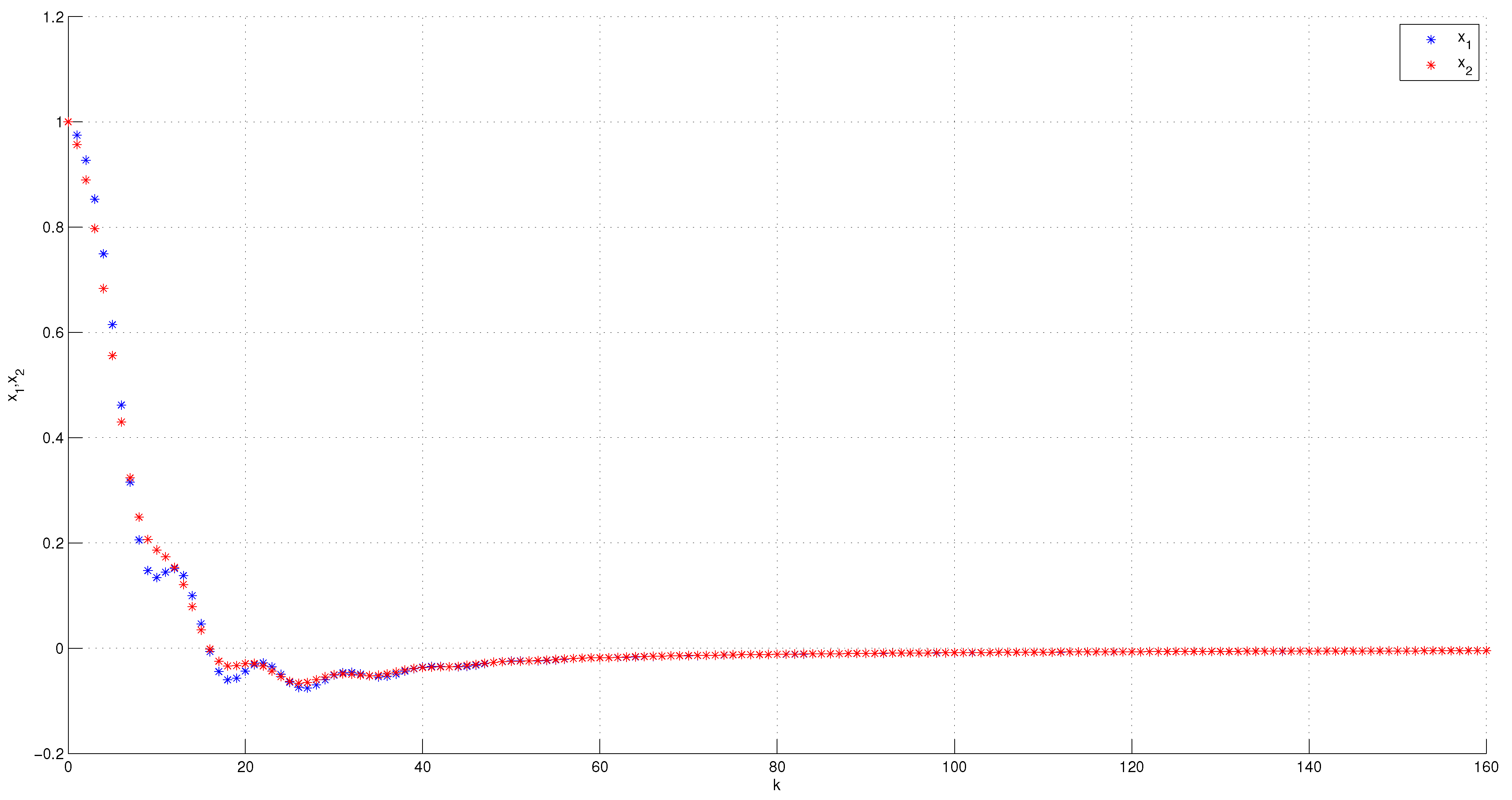
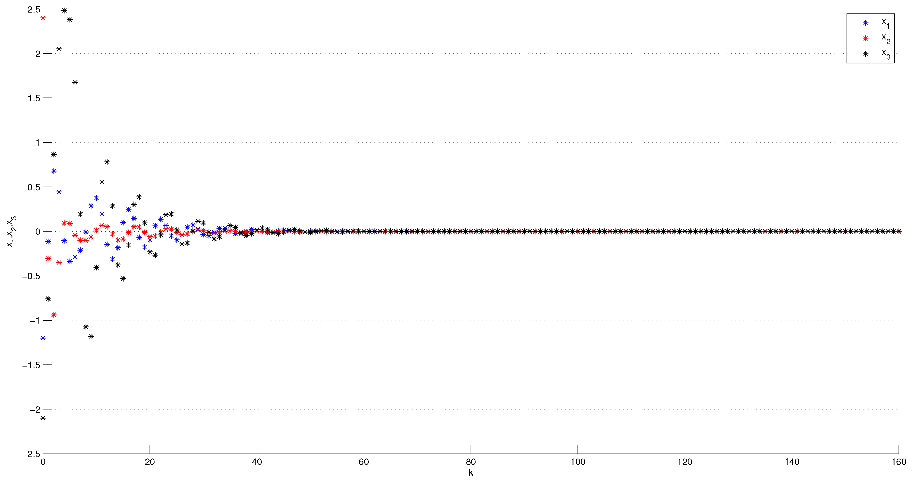
4. Illustrative Numerical Examples

In the interests of verifying the theoretical stability results of the solutions of the incommensurate h-nabla FoDSs, two numerical examples are provided in the forthcoming content.

Example 1.

Consider the following system:

$$\left\{\begin{array}{c}{}_0^C{\nabla }_1^{\frac{1}{2}}{x}_1\left(k\right)=-1.01sin\left(x_1\left(k\right)\right)+0.98sin\left(x_2\left(k\right)\right),\hfill \\ {}_0^C{\nabla }_1^{\frac{1}{4}}{x}_2\left(k\right)=0.48x_2\left(k\right)cos\left(x_1\left(k\right)\right)-0.56x_1\left(k\right)cos\left(x_2\left(k\right)\right).\hfill \end{array}\right.$$

(26)

One can verify that the origin represents an equilibrium point of the above system. In addition, the Jacobian matrix J of this system can be obtained to be in the following form:

$$J=\frac{\partial f(0,0)}{\partial x}=\left(\begin{array}{cc}\frac{\partial f_1(0,0)}{\partial x_1}& \frac{\partial f_1(0,0)}{\partial x_2}\\ \frac{\partial f_2(0,0)}{\partial x_1}& \frac{\partial f_2(0,0)}{\partial x_2}\end{array}\right)=\left(\begin{array}{cc}-1.01& 0.98\\ -0.56& 0.48\end{array}\right).$$

In this case, we can obtain $M=4$, and therefore

$$det\left(\left(\begin{array}{cc}{\lambda }^2& 0\\ 0& \lambda \end{array}\right)-\left(\begin{array}{cc}-1.01& 0.98\\ -0.56& 0.48\end{array}\right)\right)=0,$$

⇔

$${\lambda }^3-0.48{\lambda }^2+1.01\lambda +0.064=0.$$

(27)

Consequently, the solution of the above equation will be as follows:

$$\begin{array}{c}{\lambda }_1=-6.1349\times {10}^{-2},\hfill \\ {\lambda }_2=0.27067-0.98486i,\hfill \\ {\lambda }_3=0.27067+0.98486i.\hfill \end{array}$$

Clearly, it can be inferred that ${\lambda }_i\in \mathbb{C}\setminus K^{\frac{1}{4}}$, for $1\le i\le 3$. Therefore, in light of Corollary 2, we can conclude that the zero solution of system (26) is locally asymptotically stable. For the purpose of demonstrating the accuracy of this result, we plot Figure 1, which confirms that the states of the solution of system (26) are indeed convergent to the origin, asserting that such solution is stable.

Figure 1. The stability of the trivial solution of system (26) with $x_1\left(0\right)=x_2\left(0\right)=1$.

Example 2.

Consider the following system:

$$\left\{\begin{array}{c}{}_0^C{\nabla }_1^{\frac{1}{2}}{x}_1\left(k\right)=-0.98sin\left(x_1\left(k\right)\right)-0.2sin\left(x_3\left(k\right)\right),\hfill \\ {}_0^C{\nabla }_1^{\frac{1}{3}}{x}_2\left(k\right)=0.2x_1\left(k\right)-1.01x_2\left(k\right)+0.02x_3\left(k\right),\hfill \\ {}_0^C{\nabla }_1^{\frac{2}{3}}{x}_3\left(k\right)=0.4sin\left(x_1\left(k\right)\right)+\frac{x_2^2\left(k\right)}{1+x_2^2\left(k\right)}-sin\left(x_3\left(k\right)\right).\hfill \end{array}\right.$$

(28)

To deal with the above system, it should be noted that the origin $(0,0,0)$ represents an equilibrium point. Furthermore, the Jacobian matrix J of such a system can be obtained as follows:

$$J=\left(\begin{array}{ccc}-0.98& 0& -0.2\\ 0.2& -1.01& 0.02\\ 0.4& 0& -1\end{array}\right).$$

Herein, $M=6$ and so

$$det\left(\left(\begin{array}{ccc}{\lambda }^3& 0& 0\\ 0& {\lambda }^2& 0\\ 0& 0& {\lambda }^4\end{array}\right)-\left(\begin{array}{ccc}-0.98& 0& -0.2\\ 0.2& -1.01& 0.02\\ 0.4& 0& -1\end{array}\right)\right)=0,$$

⇔

$${\lambda }^9+1.01{\lambda }^7+0.98{\lambda }^6+{\lambda }^5+0.9898{\lambda }^4+1.01{\lambda }^3+1.06{\lambda }^2+1.0706=0.$$

(29)

It follows that the solution of (29) has the form:

$$\begin{array}{cc}{\lambda }_1=\hfill & -1.0065\\ {\lambda }_2=\hfill & -1.0050i\\ {\lambda }_3=\hfill & 1.0050i\\ {\lambda }_4=\hfill & 0.48524-0.88198i\\ {\lambda }_5=\hfill & 0.48524+0.88198i\\ {\lambda }_6=\hfill & 0.72916+0.69826i\\ {\lambda }_7=\hfill & 0.72916-0.69826i\\ {\lambda }_8=\hfill & -0.71118-0.71688i\\ {\lambda }_9=\hfill & -0.71118+0.71688i.\end{array}$$

Accordingly, we can conclude that ${\lambda }_i\in \mathbb{C}\setminus K^{\frac{1}{6}}$, for $1\le i\le 9$. Again, based on Corollary 2, we can conclude that the zero solution of system (28) is locally asymptotically stable. To verify this inference, we plot Figure 2, which demonstrates the stability of that solution at zero.

Figure 2. The stability of the trivial solution of system (28) with $x_1\left(0\right)=-1.2,x_2\left(0\right)=2.4,x_3\left(0\right)=-2.1$.

5. Conclusions

In the presented work, a study on the stability analysis of linear and nonlinear incommensurate h-nabla fractional-order difference systems has been provided. Numerous stability results regarding these systems have been inferred and then verified numerically via two illustrative numerical simulations.

References

1. Liu, X.; Jia, B.; Erbe, L.; Peterson, A. Stability analysis for a class of nabla (q; h)-fractional difference equations. Turk. J. Math. 2019, 43, 664–687. [Google Scholar] [CrossRef]
2. Matignon, D. Stability properties for generalized fractional differential systems. ESAIM Proc. 1998, 5, 145–158. [Google Scholar] [CrossRef] [Green Version]
3. Li, Y.; Chen, Y.Q.; Podlubny, I. Mittag–Leffler stability of fractional order nonlinear dynamic systems. Automatica 2009, 45, 1965–1969. [Google Scholar] [CrossRef]
4. Li, Y.; Chen, Y.Q.; Podlubny, I. Stability of fractional-order nonlinear dynamic systems: Lyapunov direct method and generalized Mittag–Leffler stability. Comput. Math. Appl. 2010, 59, 1810–1821. [Google Scholar] [CrossRef] [Green Version]
5. Čermák, J.; Nechvátal, L. On (q; h)-analogue of fractional calculus. J. Nonlinear Math. Phys. 2010, 17, 51–68. [Google Scholar] [CrossRef] [Green Version]
6. Čermák, J.; Tomáš, K.; Nechvátal, L. Discrete Mittag–Leffler functions in linear fractional difference equations. Abstr. Appl. Anal. 2011, 2011, 565067. [Google Scholar] [CrossRef] [Green Version]
7. Du, F.F.; Erbe, L.; Jia, B.G.; Peterson, A.C. Two asymptotic results of solutions for Nabla fractional (q; h)-difference equations. Turk. J. Math. 2018, 42, 2214–2242. [Google Scholar] [CrossRef]
8. Du, F.F.; Jia, B.G.; Erbe, L.; Peterson, A.C. Monotonicity and convexity for nabla fractional (q; h)-differences. J. Differ. Equ. Appl. 2016, 22, 1124–1243. [Google Scholar] [CrossRef]
9. Jia, B.G.; Chen, S.Y.; Erbe, L.; Peterson, A. Liapunov functional and stability of linear nabla (q; h)-fractional difference equations. J. Differ. Equ. Appl. 2017, 23, 1974–1985. [Google Scholar] [CrossRef]
10. Segi Rahmat, M.R. The (q; h)-Laplace transform on discrete time scales. Comput. Math. Appl. 2011, 62, 272–281. [Google Scholar] [CrossRef] [Green Version]
11. Segi Rahmat, M.R.; Noorani, M.S. Caputo type fractional difference operator and its application on discrete time scales. Adv. Differ. Equ. 2015, 2015, 160. [Google Scholar] [CrossRef] [Green Version]
12. Fernandez-Anaya, G.; Nava-Antonio, G.; Jamous-Galante, J.; Munoz-Vega, R.; Hernández-Martínez, E.G. Lyapunov functions for a class of nonlinear systems using Caputo derivative. Commun. Nonlinear Sci. Numer. Simul. 2017, 43, 91–99. [Google Scholar] [CrossRef]
13. Djenina, N.; Ouannas, A.; Batiha, I.M.; Grassi, G.; Pham, V.-T. On the Stability of Linear Incommensurate Fractional-Order Difference Systems. Mathematics 2020, 8, 1754. [Google Scholar] [CrossRef]
14. Elaydi, S.; Murakami, S. Asymptotic stability versus exponential stability in linear volterra difference equations of convolution type. J. Differ. Equ. Appl. 1996, 940, 35–46. [Google Scholar] [CrossRef] [Green Version]
15. Shatnawi, M.T.; Djenina, N.; Ouannas, A.; Batiha, I.M.; Grassi, G. Novel convenient conditions for the stability of nonlinear incommensurate fractional-order difference systems. Alex. Eng. J. 2022, 61, 1655–1663. [Google Scholar] [CrossRef]
16. Talbi, I.; Ouannas, A.; Khennaoui, A.A.; Berkane, A.; Batiha, I.M.; Grassi, G.; Pham, V.T. Different dimensional fractional-order discrete chaotic systems based on the Caputo h-difference discrete operator: Dynamics, control, and synchronization. Adv. Differ. Equ. 2020, 2020, 624. [Google Scholar] [CrossRef]
17. Khennaoui, A.A.; Ouannas, A.; Momani, S.; Batiha, I.M.; Dibi, Z.; Grassi, G. On Dynamics of a Fractional-Order Discrete System with Only One Nonlinear Term and without Fixed Points. Electronics 2020, 9, 2179. [Google Scholar] [CrossRef]
18. Khennaoui, A.A.; Othman Almatroud, A.; Ouannas, A.; Mossa Al-sawalha, M.; Grassi, G.; Pham, V.T.; Batiha, I.M. An Unprecedented 2-Dimensional Discrete-Time Fractional-Order System and Its Hidden Chaotic Attractors. Math. Probl. Eng. 2021, 2021, 6768215. [Google Scholar] [CrossRef]
19. Batiha, I.M.; Ouannas, A.; Emwas, J.A. A stabilization approach for a novel chaotic fractional-order discrete neural network. J. Math. Comput. Sci. 2021, 11, 5514–5524. [Google Scholar]
20. Suwan, I.; Owies, S.; Abdeljawad, T. Monotonicity results for h-discrete fractional operators and application. Adv. Differ. Equ. 2018, 2018, 207. [Google Scholar] [CrossRef]
21. Čermák, J.; Nechvátal, L. On a problem of linearized stability for fractional difference equations. Nonlinear Dyn. 2021, 10, 1253–1267. [Google Scholar] [CrossRef]