Article

Numerical Solutions of Third-Order Time-Fractional Differential Equations Using Cubic B-Spline Functions

1
Department of Mathematics, University of Sargodha, Sargodha 40100, Pakistan
2
Department of Mathematics and Statistics, College of Science, Taif University, P.O. Box 11099, Taif 21944, Saudi Arabia
3
Department of Mathematics, Division of Science and Technology, University of Education, Lahore 54770, Pakistan
4
Department of Mathematics, University of the Punjab, Lahore 54590, Pakistan
*
Author to whom correspondence should be addressed.
Fractal Fract. 2022, 6(9), 528; https://doi.org/10.3390/fractalfract6090528
Submission received: 17 August 2022 / Revised: 9 September 2022 / Accepted: 13 September 2022 / Published: 17 September 2022

Abstract

:
Numerous fields, including the physical sciences, social sciences, and earth sciences, benefit greatly from the application of fractional calculus (FC). The fractional-order derivative is developed from the integer-order derivative, and in recent years, real-world modeling has performed better using the fractional-order derivative. Due to the flexibility of B-spline functions and their capability for very accurate estimation of fractional equations, they have been employed as a solution interpolating polynomials for the solution of fractional partial differential equations (FPDEs). In this study, cubic B-spline (CBS) basis functions with new approximations are utilized for numerical solution of third-order fractional differential equation. Initially, the CBS functions and finite difference scheme are applied to discretize the spatial and Caputo time fractional derivatives, respectively. The scheme is convergent numerically and theoretically as well as being unconditionally stable. On a variety of problems, the validity of the proposed technique is assessed, and the numerical results are contrasted with those reported in the literature.

1. Introduction

The more generalzed variant of classical calculus is fractional calculus. FC has implementations in physics, natural science, fluid mechanics, electricity swaption, mathematical biology, and certain other fields [1,2]. Fractional differential equations have sparked a lot of interest due to their appearance in various disciplines. Fractional differential equation (FDE) models are considered to be more reliable for the explanation of particular systems. Numerous physical models have been expanded in the form of FDEs in the past years. The FDEs have been discovered to be pertinent models for some physical processes in astro-physics, fractal networks, signal processing, chaotic dynamics, turbulence, continuum mechanics, and wave propagation [3,4,5,6,7]. FDEs were viewed as a challenge by many researchers, who discovered numerical solutions. Researchers have focused on finding numerical and true solutions to FDEs because of their growing applicability. Finding numerical solutions is necessary since it is difficult to solve an FDE analytically. Numerous numerical techniques can be found in the literature [8,9].
In this work, we will look into the following problem [10]:
3 w ( ψ , t ) t 3 + κ 2 w ( ψ , t ) t 2 + 0 C D t γ w ( ψ , t ) + w ( ψ , t ) υ 2 w ( ψ , t ) ψ 2 = f ( ψ , t ) , ψ [ 0 , L ] , t [ 0 , T 0 ] ,
with initial and boundary conditions:
w ( ψ , 0 ) = g 1 ( ψ ) , w t ( ψ , 0 ) = g 2 ( ψ ) , w t t ( ψ , 0 ) = g 3 ( ψ ) , ψ [ 0 , L ] , w ( 0 , t ) = r 1 ( t ) , w ( L , t ) = r 2 ( t ) , t [ 0 , T 0 ] .
Here, 0 < γ 1 is a fractional order, κ > 0 , υ > 0 are parameters, g 1 ( ψ ) , g 2 ( ψ ) , r 1 ( t ) , r 2 ( t ) are known functions, f ( ψ , t ) is a source term, and w ( ψ , t ) is an unknown function. Equation (1) is called the third-order linear time-varying dynamical system [11] when γ = 1 . Moreover, 0 C D t γ symbolizes the Caputo fractional derivative (CFD) and is explained as:
0 C D t γ w ( ψ , t ) = 1 Γ ( n γ ) 0 t w ψ , ξ ξ d ξ t ξ γ n + 1 , n 1 < γ n , n N , n w ψ , t t n , γ = n .
where Γ is the Euler’s Gamma function.
Fractional derivatives have a better level of elasticity in the model and yield useful tool for describing the history of variable and hereditary features in a variety of dynamical systems. Khalid et al. [12] have examined the computational study of the Caputo time fractional Allen– Cahn equation. Wu et al. [13] have described the fractional impulsive differential equations including the analytical solutions and short memory cases. The new fractional operator in the Caputo perspective is a extension of the conventional proportional derivative introduced by [14], which has a wide range of advantages in control theory. Caputo has made a significant contribution to fractional calculus and its applications [15,16]. The foremost benefit of Caputo fractional derivatives is its capability to include conventional, initial, and boundary conditions in the problem. The Caputo derivative of a constant function is zero.
B-spline maintains a high level of smoothness at the domain’s knots. Many researchers have presented novel schemes based on B-splines for the solutions of FPDEs. Akram et al. [17] applied extended cubic B-spline (ECBS) functions on time-fractional telegraph equations in the Caputo sense for its numerical modeling. These functions offer continuous solutions and very accurate approximations to exact solutions over the spatial domain. A spline function has been employed by numerous researchers to solve the fractional differential equations because of its simplicity, acceptable approximation, compact support and obtained solutions in piecewise polynomial format having a continuity of order two [18,19], and it can also approximate the optimal solution of FPDEs of any order.
The proposed study can be arranged as follows: In Section 2, the cubic B-spline basis functions and new approximation for second derivatives are presented. Discretization of the time derivative is presented in Section 3. The methodology of the proposed problem is discussed in Section 4. The stability and convergence of the presented scheme are analyzed in Section 5. Numerical implementation via two test problems is discussed in Section 5. Finally, the results of the preferred technique are shown in Section 6.

2. Cubic B-Spline Functions

To describe CBS functions, let us further expand [a,b] to [ a 3 h , b + 3 h ] with equidistant knots ψ m = a + m h ; m = 3 , 2 , , M ˜ + 3 . The classical CBS functions can be defined as [20]:
B m * ( ψ ) = 1 6 h 3 ( ψ ψ m 2 ) 3 , ψ [ ψ m 2 , ψ m 1 ] h 3 + 3 h 2 ( ψ ψ m 1 ) + 3 h ( ψ ψ m 1 ) 2 3 ( ψ ψ m 1 ) 3 , ψ [ ψ m 1 , ψ m ] h 3 + 3 h 2 ( ψ m + 1 ψ ) + 3 h ( ψ m + 1 ψ ) 2 3 h ( ψ m + 1 ψ ) 3 , ψ [ ψ m , ψ m + 1 ] ( ψ m + 2 ψ ) 3 , ψ [ ψ m + 1 , ψ m + 2 ] 0 , otherwise ,
where m = 1 : 1 : M ˜ + 1 . For any twice-differentiable function w ( ψ , t ) , there exists a unique third-degree B-spline approximate solution W ( ψ , t ) , which can be written as:
W ( ψ , t ) = m = 1 M ˜ + 1 ϱ m ( t ) B m * ( ψ ) ,
where ϱ m ( t ) are unknowns to be evaluated. We demonstrate the CBS approximation for w and its first two space derivatives, at m t h knot, by W m , W ˙ m , W ¨ m , respectively:
W m = p = m 1 m + 1 ϱ p B p * ( ψ m ) = ( c 1 ϱ m 1 + c 2 ϱ m + c 1 ϱ m + 1 ) ,
W ˙ m = p = m 1 m + 1 ϱ p B ˙ p * ( ψ m ) = ( c 3 ϱ m 1 + c 3 ϱ m + 1 ) ,
W ¨ m = p = m 1 m + 1 ϱ p B ¨ p * ( ψ m ) = ( c 4 ϱ m 1 + c 5 ϱ m + c 4 ϱ m + 1 ) ,
where c 1 = 1 6 , c 2 = 4 6 , c 3 = 1 2 h , c 4 = 1 h 2 , c 5 = 2 h 2 . Moreover, from (6)–(8), we can establish the following expressions [21]:
W ˙ m = w ( ψ m ) h 4 180 w ( 5 ) ( ψ m ) + ,
W ¨ m = w ( ψ m ) h 2 12 w ( 4 ) ( ψ m ) + h 4 360 w ( 6 ) ( ψ m ) +

New Approximation for W ¨ m

The truncation error in W ¨ m is O ( h 2 ) . Therefore, instead of using (8), we shall apply the following O ( h 3 ) approximation for a second-order derivative [22,23]:
W ¨ m = 1 12 h 2 14 ϱ 1 33 ϱ 0 + 28 ϱ 1 14 ϱ 2 + 6 ϱ 3 ϱ 4 , for m = 0 , ϱ m 2 + 8 ϱ m 1 18 ϱ m + 8 ϱ m + 1 + ϱ m + 2 , for m = 1 : 1 : M ˜ 1 , ϱ M ˜ 4 + 6 ϱ M ˜ 3 14 ϱ M ˜ 2 + 28 ϱ M ˜ 1 33 ϱ M ˜ + 14 ϱ M ˜ + 1 , for m = M ˜ .

3. Temporal Discretization

By utilizing the forward finite difference approach, the Caputo time fractional derivative is discretized. Suppose t j = j τ , j = 0 , 1 , , K in which τ = T 0 K is the step size in time direction. The time fractional derivative at knot t = t j in the Caputo sense can be approximated as [23]:
γ w ( ψ , t j + 1 ) t γ = 1 Γ ( 1 γ ) o t w ( ψ , Y ) Y d Y ( t j + 1 Y ) γ , = 1 Γ ( 1 γ ) s = 0 j s τ ( s + 1 ) τ w ( ψ , Y ) Y d Y ( t j + 1 Y ) γ , = 1 Γ ( 1 γ ) s = 0 j w ( ψ , t s + 1 ) w ( ψ , t s ) τ s τ ( s + 1 ) τ d Y ( t j + 1 Y ) γ + e ˘ τ j + 2 , = 1 Γ ( 1 γ ) s = 0 j w ( Y , t j s + 1 ) w ( Y , t j s ) τ s τ ( s + 1 ) τ d Φ Φ γ + e ˘ τ j + 2 .
The above expression becomes:
γ w ( ψ , t j + 1 ) t γ = 1 Γ ( 2 γ ) s = 0 j d ˇ s w ( ψ , t j s + 1 ) w ( ψ , t j s ) τ γ + e ˘ τ j + 2 ,
where d ˇ s = ( s + 1 ) 1 γ s 1 γ . The truncation error e ˘ τ j + 2 is bounded [24], i.e.,
| e ˘ τ j + 2 | = c ´ τ 2 γ ,
where c ´ is the constant.
Lemma 1.
The coefficients d ˇ s have the following properties [25]:
  • d ˇ s > 0 for s = 0 , 1 , 2 , , j ;
  • d ˇ 0 = 1 ;
  • d ˇ 0 > d ˇ 1 > d ˇ 2 > . . . > d ˇ s , d ˇ s 0 a s s ;
  • s = 0 j ( d ˇ s d ˇ s + 1 ) + d ˇ j + 1 = ( 1 d ˇ 1 ) + s = 1 j 1 ( d ˇ s d ˇ s + 1 ) + d ˇ j = 1 .

4. Description of Numerical Method

By using the new cubic B-spline collocation method, the numerical solution of the time-fractional differential equation of the third order is obtained. The ϑ -weighted scheme is applied to (1) in order to obtain the following approximation:
( 3 w t 3 ) j + κ ( 2 w t 2 ) j + ( 0 c D t γ w ) j + 1 = ϑ υ ( 2 w ψ 2 ) j + 2 ϑ ( w ) j + 2 + ( 1 ϑ ) υ ( 2 w ψ 2 ) j + 1 ( 1 ϑ ) ( w ) j + 1 + f j + 2 ,
where 0 ϑ 1 , j, j + 1 , and j + 2 are successive time levels j = 0 , 1 , 2 , . By discretizing the time derivatives and approximation of the third-order fractional derivative used in (12), we obtain:
W m j + 2 3 W m j + 1 + 3 W m j W m j 1 τ 3 + κ W m j + 1 2 W m j + W m j 1 τ 2 + τ γ Γ ( 2 γ ) s = 0 j d ˇ s W m j s + 1 W m j s = ϑ ( υ ( W ψ ψ ) m j + 2 W m j + 2 ) + ( 1 ϑ ) ( υ ( W ψ ψ ) m j + 1 W m j + 1 ) + f j + 2 ,
After some simplification, we have:
W m j + 2 3 W m j + 1 + 3 W m j W m j 1 + κ τ ( W m j + 1 2 W m j + W m j 1 ) + τ 3 γ Γ ( 2 γ ) s = 0 j b ˇ s W m j s + 1 W m j s = τ 3 ϑ ( υ ( W ψ ψ ) m j + 2 W m j + 2 ) + τ 3 ( 1 ϑ ) ( υ ( W ψ ψ ) m j + 1 W m j + 1 ) + τ 3 f j + 2 ,
where r = τ 3 γ Γ ( 2 γ ) . The above equation can be rewritten as:
( 1 + τ 3 ϑ ) W m j + 2 υ τ 3 ϑ ( W ψ ψ ) m j + 2 = ( 3 τ κ τ 3 ( 1 ϑ ) r ) W m j + 1 + υ τ 3 ( 1 ϑ ) ( W ψ ψ ) m j + 1 + ( 2 κ τ 3 + r ) W m j + ( 1 κ τ ) W m j 1 r s = 1 j d ˇ s W m j s + 1 W m j s + τ 3 f j + 2 .
It is noted that the scheme is explicit when ϑ = 0 , the scheme is fully implicit for ϑ = 1 , and for ϑ = 1 2 , the approach is the Crank–Nicholson approach. Here, we use the Crank–Nicholson scheme:
( 1 + τ 3 2 ) W m j + 2 υ τ 3 2 ( W ψ ψ ) m j + 2 = ( 3 τ κ τ 3 2 r ) W m j + 1 + υ τ 3 2 ( W ψ ψ ) m j + 1 + ( 2 κ τ 3 + r ) W m j + ( 1 κ τ ) W m j 1 r s = 1 j d ˇ s W m j s + 1 W m j s + τ 3 f j + 2 .
We use (6), (7), and (11) in (15) for m = 0 , 1 , 2 , 3 , , M ˜ . This method includes ( M ˜ + 1 ) linear equations with ( M ˜ + 3 ) unknowns. In order to obtain the two additional equations and the unique solution to the problem, we employ the boundary conditions. This ( M ˜ + 3 ) × ( M ˜ + 3 ) dimension matrix structure is a tridiagonal matrix.
For m = 0 , we have:
( 1 + τ 3 2 ) 1 6 ϱ 1 j + 2 + 4 6 ϱ 0 j + 2 + 1 6 ϱ 1 j + 2 υ τ 3 2 14 ϱ 1 j + 2 33 ϱ 0 j + 2 + 28 ϱ 1 j + 2 14 ϱ 2 j + 2 + 6 ϱ 3 j + 2 ϱ 4 j + 2 = 3 κ τ τ 3 2 r 1 6 ϱ 1 j + 1 + 4 6 ϱ 0 j + 1 + 1 6 ϱ 1 j + 1 + υ τ 3 2 14 ϱ 1 j + 1 33 ϱ 0 j + 1 + 28 ϱ 1 j + 1 14 ϱ 2 j + 1 + 6 ϱ 3 j + 1 ϱ 4 j + 1 + ( 2 κ τ 3 + r ) 1 6 ϱ 1 j + 4 6 ϱ 0 j + 1 6 ϱ 1 j + ( 1 κ τ ) 1 6 ϱ 1 j 1 + 4 6 ϱ 0 j 1 + 1 6 ϱ 1 j 1 r s = 1 j d ˇ s 1 6 ϱ 1 j s + 1 + 4 6 ϱ 0 j s + 1 + 1 6 ϱ 1 j s + 1 1 6 ϱ 1 j s + 4 6 ϱ 0 j s + 1 6 ϱ 1 j s + τ 3 f j + 2 ,
For m = 1 , 2 , 3 , , M ˜ 1 , we have:
( 1 + τ 3 2 ) 1 6 ϱ m 1 j + 2 + 4 6 ϱ m j + 2 + 1 6 ϱ m + 1 j + 2 υ τ 3 2 ϱ m 2 j + 2 + 8 ϱ m 1 j + 2 18 ϱ m j + 2 + 8 ϱ m + 1 j + 2 + ϱ m + 2 j + 2 = 3 κ τ τ 3 2 r 1 6 ϱ m 1 j + 1 + 4 6 ϱ m j + 1 + 1 6 ϱ m + 1 j + 1 + υ τ 3 2 ϱ m 2 j + 1 + 8 ϱ m 1 j + 1 18 ϱ m j + 1 + 8 ϱ m + 1 j + 1 + ϱ m + 2 j + 1 + 2 κ τ 3 + r 1 6 ϱ m 1 j + 4 6 ϱ m j + 1 6 ϱ m + 1 j + ( 1 κ τ ) 1 6 ϱ m 1 j 1 + 4 6 ϱ m j 1 + 1 6 ϱ m + 1 j 1 r s = 1 j d ˇ s 1 6 ϱ m 1 j s + 1 + 4 6 ϱ m j s + 1 + 1 6 ϱ m + 1 j s + 1 1 6 ϱ m 1 j s + 4 6 ϱ m j s + 1 6 ϱ m + 1 j s + τ 3 f j + 2 ,
For m = M ˜ , we have:
( 1 + τ 3 2 ) 1 6 ϱ M ˜ 1 j + 2 + 4 6 ϱ M ˜ j + 2 + 1 6 ϱ M ˜ + 1 j + 2 υ τ 3 2 ϱ M ˜ 4 j + 2 + 6 ϱ M ˜ 3 j + 2 14 ϱ M ˜ 2 j + 2 + 28 ϱ M ˜ 1 j + 2 33 ϱ M ˜ j + 2 + 14 ϱ M ˜ + 1 j + 2 = 3 κ τ τ 3 2 r 1 6 ϱ M ˜ 1 j + 1 + 4 6 ϱ M ˜ j + 1 + 1 6 ϱ M ˜ + 1 j + 1 + υ τ 3 2 ( ϱ M ˜ 4 j + 1 + 6 ϱ M ˜ 3 j + 1 14 ϱ M ˜ 2 j + 1 + 28 ϱ M ˜ 1 j + 1 33 ϱ M ˜ j + 1 + 14 ϱ M ˜ + 1 j + 1 ) + ( 2 κ τ 3 + r ) 1 6 ϱ M ˜ 1 j + 4 6 ϱ M ˜ j + 1 6 ϱ M ˜ + 1 j + ( 1 κ τ ) 1 6 ϱ M ˜ 1 j 1 + 4 6 ϱ M ˜ j 1 + 1 6 ϱ M ˜ + 1 j 1 r s = 1 j d ˇ s 1 6 ϱ M ˜ 1 j s + 1 + 4 6 ϱ M ˜ j s + 1 + 1 6 ϱ M ˜ + 1 j s + 1 1 6 ϱ M ˜ 1 j s + 4 6 ϱ M ˜ j s + 1 6 ϱ M ˜ + 1 j s + τ 3 f j + 2 .

Initial Vector

For the iteration process, the initial solution vectors must be identified at the two boundaries with the help of the initial conditions and their derivatives:
1.
( W n 0 ) ψ = d d ψ g 1 ( ψ m ) , m = 0 ;
2.
W n 0 = g 1 ( ψ m ) , m = 0 , 1 , M ˜ ;
3.
( W n 0 ) ψ = d d ψ g 1 ( ψ m ) , m = M ˜ .
For j = 0 , this yields a ( M ˜ + 3 ) × ( M ˜ + 3 ) matrix system of the form:
Q ϱ 0 = d ,
where
ϱ 0 = ϱ 3 0 , ϱ 2 0 , ϱ 1 0 , , ϱ M ˜ 1 0 T , d = g 1 ( ψ 0 ) , g 1 ( ψ 0 ) , , g 1 ( ψ M ˜ ) , g 1 ( ψ M ˜ ) T ,
and Q denotes the coefficient matrix of order ( M ˜ + 3 ) × ( M ˜ + 3 ) , which can be written as:
c 3 0 c 3 0 c 1 c 2 c 1 0 0 c 1 c 2 c 1 c 1 c 2 c 1 0 c 3 0 c 3 .
From the other initial conditions, by using finite forward difference scheme, we obtain:
( W t ) m 0 = g 2 ( ψ m ) , m = 0 , 1 , M ˜ , ( W t ) m 0 = ( W ) m 1 ( W ) m 0 τ , ( W ) m 1 ( W ) m 0 τ = g 2 ( ψ m ) , ( W ) m 1 = τ g 2 ( ψ m ) + ( W ) m 0 .
Similarly,
( W t t ) m 0 = g 3 ( ψ m ) , ( W t t ) m 0 = ( W ) m 2 2 ( W ) m 1 + ( W ) m 0 τ 2 = g 3 ( ψ m ) , ( W ) m 2 = τ 2 g 3 ( ψ m ) + ( 2 ( W ) m 1 ( W ) m 0 ) .
We obtain ϱ j = ϱ 3 j , ϱ 2 j , ϱ 1 j , , ϱ M ˜ 1 j for j = 1 , 2 from Equations (20) and (21), respectively.

5. Stability and Convergence Analyses

In this section, stability and convergence analyses of the proposed technique are presented.

5.1. Stability Analysis

To analyze the stability of existing method, the von Neumann technique is used. Assume that the Fourier series representing the different expression is:
ϕ l j = w ( ψ l , t j ) W l j = ς j exp i l φ h ,
where i = 1 . φ and h are the mode number and moving scale in space direction, respectively. We obtain the following relation by applying (22) in (15):
( 1 + τ 3 2 ) φ l j + 2 υ τ 3 2 ( φ ψ ψ ) l j + 2 = ( 3 κ τ τ 3 2 r ) φ l j + 1 + υ τ 3 2 ( φ ψ ψ ) l j + 1 + ( 2 κ τ 3 + r ) φ l j + ( 1 κ τ ) φ l j 1 r s = 1 j d ˇ s φ l j s + 1 ϕ l j s .
The Equation (23) is explained as:
( 1 + τ 3 2 ) ς j + 2 1 6 e i ( l 1 ) φ h + 4 6 e i ( l ) φ h + 1 6 e i ( l + 1 ) φ h υ τ 3 2 ς j + 2 ( e i ( l 2 ) φ h + 8 e i ( l 1 ) φ h 18 e i ( l ) φ h + 8 e i ( l + 1 ) φ h + e i ( l + 2 ) φ h ) = 3 κ τ τ 3 2 r ς j + 1 1 6 e i ( l 1 ) φ h + 4 6 e i ( l ) φ h + 1 6 e i ( l + 1 ) φ h + υ τ 3 2 ς j + 1 e i ( l 2 ) φ h + 8 e i ( l 1 ) φ h 18 e i ( l ) φ h + 8 e i ( l + 1 ) φ h + e i ( l + 2 ) φ h + 2 κ τ 3 + r ς j ( 1 6 e i ( l 1 ) φ h + 4 6 e i ( l ) φ h + 1 6 e i ( l + 1 ) φ h ) + ( 1 κ τ ) ς j 1 1 6 e i ( l 1 ) φ h + 4 6 e i ( l ) φ h + 1 6 e i ( l + 1 ) φ h r s = 1 j d ˇ s ς j s + 1 1 6 e i ( l 1 ) φ h + 4 6 e i ( l ) φ h + 1 6 e i ( l + 1 ) φ h ς j s 1 6 e i ( l 1 ) φ h + 4 6 e i ( l ) φ h + 1 6 e i ( l + 1 ) φ h .
Rearranging the above equation, we obtain:
1 + τ 3 2 ς j + 2 2 6 cos ( φ h ) + 4 6 υ τ 3 2 ς j + 2 2 cos ( 2 φ h ) + 16 cos ( φ h ) 18 = 3 κ τ τ 3 2 r ς j + 1 2 6 cos ( φ h ) + 4 6 + υ τ 3 2 ς j + 1 2 cos ( 2 φ h ) + 16 cos ( φ h ) 18 + 2 κ τ 3 + r ζ j 2 6 cos ( φ h ) + 4 6 + 1 κ τ ς j 1 2 6 cos ( φ h ) + 4 6 r s = 1 j d ˇ s ς j s + 1 2 6 cos ( φ h ) + 4 6 ς j s 2 6 cos ( φ h ) + 4 6 .
After simplification, we obtain the following relation:
ς j + 2 = 1 σ ( 3 κ τ ϖ ) ς j + 1 + 1 σ ( 2 κ τ 3 + r ) ς j + 1 σ ( 1 κ τ ) ς j 1 r σ s = 1 j d ˇ s ς j s + 1 ς j s ,
where
σ = 1 + τ 3 2 υ τ 3 2 2 cos ( 2 φ h ) + 16 cos ( φ h ) + 18 2 6 cos ( φ h ) + 4 6 ,
ϖ = ( τ 3 2 + r ) + υ τ 3 2 2 cos ( 2 φ h ) + 16 cos ( φ h ) + 18 2 6 cos ( φ h ) + 4 6 .
Clearly, σ > 1 .
Proposition 1.
Let ς j + 1 , j = 0 , 1 , 2 , T 0 × L be the solution of the proposed scheme. We then have:
| ς j + 2 | < 3 | ς 1 | .
Proof. 
Here, we use the mathematical induction to prove the result. Substituting j = 0 in (24), we obtain:
ς 2 < 3 ς 1 ,
| ς 2 | < 3 | ς 1 | .
Suppose | ς j + 1 | < 3 | ς 1 | is true for j = 0 , 1 , 2 , T 0 × L 1 :
ς j + 2 = 1 σ ( 3 κ τ ϖ ) ς j + 1 + 1 σ ( 2 κ τ 3 + r ) ς j + 1 σ ( 1 κ τ ) ς j 1 r σ s = 1 j d ˇ s ς j s + 1 ς j s ,
ς j + 2 < 3 σ ( 3 κ τ ϖ ) ς 1 + 3 σ ( 2 κ τ 3 + r ) ς 1 + 3 σ ( 1 κ τ ) ζ 1 r σ s = 1 j d ˇ s 3 ς 1 3 ς 1 ,
ς j + 2 < 3 σ ( 3 κ τ ϖ ) + ( 2 κ τ 3 + r ) + ( 1 κ τ ) ς 1 = 3 σ ( 1 + r ϖ ) ς 1 ,
| ς j + 2 | < 3 σ | ς 1 | ,
| ς j + 2 | < 3 | ς 1 | .
From the above proposition, it can declared that for every j, the error of the recommended scheme at level j does not increase the initial error. Hence, the proposed scheme is stable unconditionally. □

5.2. Convergence Analysis

Theorem 1.
Let w ( ψ m , t j ) be the analytical solution of the Equations (1) and (2) and W j be the approximate solution of the assumed problem. Then,
| | E ˘ j + 2 | | S ˜ + c ´ τ 2 γ ,
where S ˜ is constant and E ˘ j + 2 = w ( ψ m , t j + 2 ) W j + 2 .
Proof. 
From the difference between the analytical and approximate solutions, we obtain:
( 1 + τ 3 2 ) E ˘ j + 2 υ τ 3 2 ( E ˘ ψ ψ ) j + 2 = ( 3 κ τ τ 3 2 r ) E ˘ j + 1 + υ τ 3 2 ( E ˘ ψ ψ ) j + 1 + ( 2 κ τ 3 + r ) E ˘ j + ( 1 κ τ ) E ˘ j 1 r s = 1 j d ˇ s E ˘ j s + 1 E ˘ j s + e ˘ τ j + 2 .
Equation (26) can be rewritten as:
( 1 + τ 3 2 ) E ˘ j + 2 υ τ 3 2 ( E ˘ ψ ψ ) j + 2 = ( 3 τ κ τ 3 2 r ) E ˘ j + 1 + υ τ 3 2 ( E ˘ ψ ψ ) j + 1 + ( 2 κ τ 3 ) E ˘ j + ( 1 κ τ ) E ˘ j 1 + r d ˇ j E ˘ 0 + r s = 0 j 1 d ˇ s d ˇ s + 1 E ˘ j s + e ˘ τ j + 2 .
For j = 0 , Equation (27) implies:
( 1 + τ 3 2 ) E ˘ 2 υ τ 3 2 ( E ˘ ψ ψ ) 2 = ( 3 κ τ τ 3 2 r ) E ˘ 1 + υ τ 3 2 ( E ˘ ψ ψ ) 1 + ( 2 κ τ 3 ) E ˘ 0 + e ˘ τ 2 .
As E ˘ 0 = 0 , we obtain:
( 1 + τ 3 2 ) E ˘ 2 , E ˘ 2 υ τ 3 2 E ˘ ψ ψ 2 , E ˘ 2 = ( 3 κ τ τ 3 2 r ) E ˘ 1 , E ˘ 2 + λ τ 3 2 E ˘ ψ ψ 1 , E ˘ 2 + e ˘ τ 2 , E ˘ 2 .
Using a ˜ x x , a ˜ = a ˜ x , a ˜ x , a ˜ , a ˜ = | | a ˜ | | 2 , a ˜ x , a ˜ = a ˜ , a ˜ x , and a ˜ , a ˜ 1 | | a ˜ | | | | a ˜ 1 | | , we obtain:
ε | | E ˘ 2 | | 2 | | E ˘ 1 | | | | E ˘ 2 | | + | | e ˘ τ 2 | | | | E ˘ 2 | | ,
where ε = ( 1 + τ 3 2 ) .
| | E ˘ 2 | | 1 ε | | E ˘ 1 | | + 1 ε | | e ˘ τ 2 | | ,
| | E ˘ | | | | E ˘ 1 | | + | | e ˘ τ 2 | | S ˜ + c ´ τ 2 γ .
Assume that (28) is true for j = 0 , 1 , , K . Taking the inner product of Equation (27) with E ˘ j + 2 , we have:
( 1 + τ 3 2 ) E ˘ j + 2 , E ˘ j + 2 υ τ 3 2 E ˘ ψ ψ j + 2 , E ˘ j + 2 = ( 3 κ τ τ 3 2 r ) E ˘ j + 1 , E ˘ j + 2 + υ τ 3 2 E ˘ ψ ψ j + 1 , E ˘ j + 2 + ( 2 κ τ 3 ) E ˘ j , E ˘ j + 2 + ( 1 κ τ ) E ˘ j 1 , E ˘ j + 2 + r s = 0 j 1 d ˇ s d ˇ s + 1 E ˘ j s , E ˘ j + 2 + e ˘ τ j + 2 , E ˘ j + 2 .
Using a ˜ x x , a ˜ = a ˜ x , a ˜ x , a ˜ x , a ˜ = a ˜ , a ˜ x , we have:
( 1 + τ 3 2 ) E ˘ j + 2 , E ˘ j + 2 = υ τ 3 2 E ˘ ψ j + 2 , E ˘ ψ j + 2 υ τ 3 2 E ˘ ψ j + 1 , E ˘ ψ j + 2 + ( 3 κ τ τ 3 2 r ) E ˘ j + 1 , E ˘ j + 2 + ( 2 κ τ 3 ) E ˘ j , E ˘ j + 2 + ( 1 κ τ ) E ˘ j 1 , E ˘ j + 2 + r s = 0 j 1 d ˇ s d ˇ s + 1 E ˘ j s , E ˘ j + 2 + e ˘ τ j + 2 , E ˘ j + 2 .
Moreover, using a ˜ , a ˜ = | | a ˜ | | 2 , a ˜ , a ˜ 1 | | a ˜ | | | | a ˜ 1 | | , we have:
( 1 + τ 3 2 ) | | E ˘ j + 2 | | ( 1 τ 3 2 r ) ( c ´ τ 2 γ ) + r s = 0 j 1 d ˇ s d ˇ s + 1 | | E ˘ j s | | + | | e ˘ τ j + 2 | | ,
| | E ˘ j + 2 | | D 1 s = 0 j 1 d ˇ s d ˇ s + 1 | | E ˘ j s | | + | | e ˘ τ j + 2 | | ,
where S ˜ j = max 0 s j 1 | | E ˘ j s | | and ε = ( 1 + τ 3 2 ) .
| | E ˘ j + 2 | | < + S ˜ j ( 1 d ˇ j ) + | | e ˘ τ j + 2 | | ,
| | E ˘ j + 2 | | < S ˜ + c ´ τ 2 γ
where S ˜ = max 0 j K S ˜ j and ( 1 d ˇ j ) < 1 . □

6. Numerical Implementation

In this section, two examples are performed in order to show the competency of the proposed scheme. The outcomes of example 1 are compared with [10]. Errors are computed using the error norm described below. The absolute error L is defined by:
L = max 0 m L w m W m ,
where w m and W m are the analytical and approximate solutions, respectively.
To compute the order of convergence ρ , the following formula can be employed:
ρ = log ( L ( K i ) ) log ( L ( K i + 1 ) ) log ( 2 ) ,
where L ( K i ) and L ( K i + 1 ) ) are the norms at knots K i and K i + 1 , respectively.
Example 1.
Consider the following third-order fractional differential equation in the Caputo sense [10]:
3 w ( ψ , t ) t 3 + κ 2 w ( ψ , t ) t 2 + 0 C D t γ w ( ψ , t ) + w ( ψ , t ) υ 2 w ( ψ , t ) ψ 2 = f ( ψ , t ) , w ( ψ , 0 ) = w t ( ψ , 0 ) = w t t ( ψ , 0 ) = 0 , 0 t 1 , w ( 0 , t ) = w ( π , t ) = 0 , 0 ψ π , 0 < γ < 1 , κ > 0 , υ > 0 .
The analytic solution of this problem is:
w ( ψ , t ) = ( 1 γ B ( γ ) t 3 + 6 γ Γ ( γ + 4 ) B ( γ ) t γ + 3 ) sin ψ ,
where B ( γ ) = 1 γ + γ Γ ( γ ) .
Table 1, Table 2 and Table 3 demonstrate the L error norm for γ = 0.001 , 0.37 , 0.5 , 0.69 , 0.81 , 0.999 and also for various values of M and K. The value of κ is different for each γ , and we choose a small parameter υ = 0.0001 for all γ . Such values of κ give minimum errors, the errors will start to increase when we increase or decrease the value of κ . Table 1 and Table 2 display the comparison of errors of proposed technique with the Crank–Nicholson finite difference method [10] for M ˜ = K = 20 and 80, respectively. It seems that the outcomes of proposed scheme are much better than results of [10]. The order of convergence can be calculated numerically and is tabulated in Table 4 and Table 5 along with the temporal and spatial directions, respectively. It is concluded that the order of convergence is almost two. The absolute error at different values of γ is displayed in Figure 1. Figure 2 depicts the 3D space–time plot of analytical and approximate solutions when γ = 0.37 , M ˜ = K = 80 . In Figure 3, Figure 4 and Figure 5, the comparison of the 3D numerical and exact solutions of proposed technique with Crank–Nicholson finite difference method (CNFDM) [10] for M ˜ = K = 20 are shown, and it is concluded that the numerical solutions of the proposed scheme are more accurate than the scheme in [10]. We may conclude that the computational findings are in good agreement with the exact solutions, demonstrating that this scheme is capable of solving the problem effectively.
Example 2.
Use the third-order FPDE (1) with
w ( ψ , 0 ) = w t ( ψ , 0 ) = w t t ( ψ , 0 ) = 0 , 0 t 1 = T 0 ,
w ( 0 , t ) = w ( 1 , t ) = 0 , 0 ψ 1 .
The exact solution is taken as w ( ψ , t ) = ( 1 + t 5 2 ) ψ 2 ( 1 ψ ) 2 , and the force function f ( ψ , t ) can be calculated with its help. The computational results of this example are given in the tables and figures at different parameter values. The absolute errors norm L is tabulated in Table 6 and Table 7 at different values of τ , h , K , M ˜ , γ and κ . The order of convergence can be calculated numerically and is tabulated in Table 8 and Table 9 along with the temporal and spatial directions, respectively. It is concluded that the order of convergence is almost two. Figure 6 displays the error plot for different values of fractional order γ . The 3D space–time graphs of the exact and numerical solutions are depicted in Figure 7, Figure 8 and Figure 9 by setting the different values of K and M ˜ . We can conclude that the results obtained by the proposed scheme are well suited with the exact solution. In addition, from these figures, we can observe that the numerical results of the present method and the exact solutions at different time stages are much closer to each other.

7. Conclusions

In the present study, we have presented cubic B-spline solutions of third-order, time-fractional, partial differential equations. The CFD has been applied to discretize the time-fractional derivative. A new approximation for the second derivative of cubic B-spline functions has been utilized in the space dimension. The given numerical algorithm has been proven to be convergent and unconditionally stable. To determine whether the presented technique is effective, two numerical test problems have been considered. Numerical results have been compared with CNFDM [10] and found that the obtained results are more accurate than [10].
The proposed method has been corroborated by certain numerical examples, which show that this new estimation is more accurate, appropriate, and valuable than previously published methods. The suggested scheme in the present study is innovative and offers a respectable level of accuracy. On the other hand, the present method will be applied on two-dimensional time fractional partial differential equations and also it is simple to use when applied to variable-order and higher-order fractional partial differential equations.

Author Contributions

Conceptualization, M.A., A.B., A.S.M.A., T.N., A.M. and G.A.; formal analysis, M.A., A.B., A.S.M.A., T.N., A.M. and G.A.; funding acquisition, M.A.; investigation, M.A.; methodology, M.A., A.B., A.S.M.A., T.N., A.M. and G.A.; software, M.A., A.B., A.M. and G.A.; supervision, M.A. and T.N.; visualization, M.A., A.B., A.S.M.A., T.N., A.M. and G.A.; writing—original draft, M.A., A.B., A.S.M.A., T.N., A.M. and G.A.; writing—review and editing, M.A., T.N., A.M. and G.A. All authors have read and agreed to the published version of the manuscript.

Funding

This research received no external funding.

Data Availability Statement

Not applicable.

Acknowledgments

The Research of Ahmed SM Alzaidi was supported by Taif University Researchers Supporting Project Number (TURSP-2020/303), Taif University, Taif, Saudi Arabia. The authors are also grateful to anonymous referees for their valuable suggestions, which significantly improved this manuscript.

Conflicts of Interest

The authors declare no conflict of interest.

References

  1. Diethelm, K.; Freed, A.D. On the solution of nonlinear fractional-order differential equations used in the modeling of viscoplasticity. Sci. Comput. Chem. Eng. 1999, 11, 217–224. [Google Scholar]
  2. Tariq, H.; Akram, G. Quintic spline technique for time fractional fourth-order partial differential equation. Numer. Methods Partial Differ. Equ. 2017, 33, 445–466. [Google Scholar] [CrossRef]
  3. Barkai, E.; Metzler, R.; Klafter, J. From continuous time random walks to the fractional Fokker-Planck equation. Phys. Rev. E 2000, 61, 132. [Google Scholar] [CrossRef] [PubMed]
  4. Van Beinum, W.; Meeussen, J.C.; Edwards, A.C.; Van Riemsdijk, W.H. Transport of ions in physically hetrogeneous systems; convection and diffusion in a column filled with alginate gel beads, predicted by a two-region model. Water Res. 2000, 34, 2043–2050. [Google Scholar] [CrossRef]
  5. Gorenflo, R.; Mainardi, F. Fractional Calculus in Fractals and Fractional Calculus in Continuum Mechanics; Springer: Vienna, Austria, 1997; pp. 291–348. [Google Scholar]
  6. Zaslavsky, G.M.; Stevens, D.; Weitzner, H. Self-similar transport in incomplete chaos. Phys. Rev. E 1993, 48, 1683. [Google Scholar] [CrossRef] [PubMed]
  7. Podlubny, I. Fractional Differential Equations; Academic Press: London, UK, 1999. [Google Scholar]
  8. Ding, Z.; Xiao, A.; Li, M. Weighted finite difference methods for a class of space fractional partial differential equations with variable coefficients. J. Comput. Appl. Math. 2010, 233, 1905–1914. [Google Scholar] [CrossRef]
  9. Yang, S.; Xiao, A.; Su, H. Convergence of the variational iteration method for solving multi-order fractional differential equations. Comput. Math. Appl. 2010, 60, 2871–2879. [Google Scholar] [CrossRef]
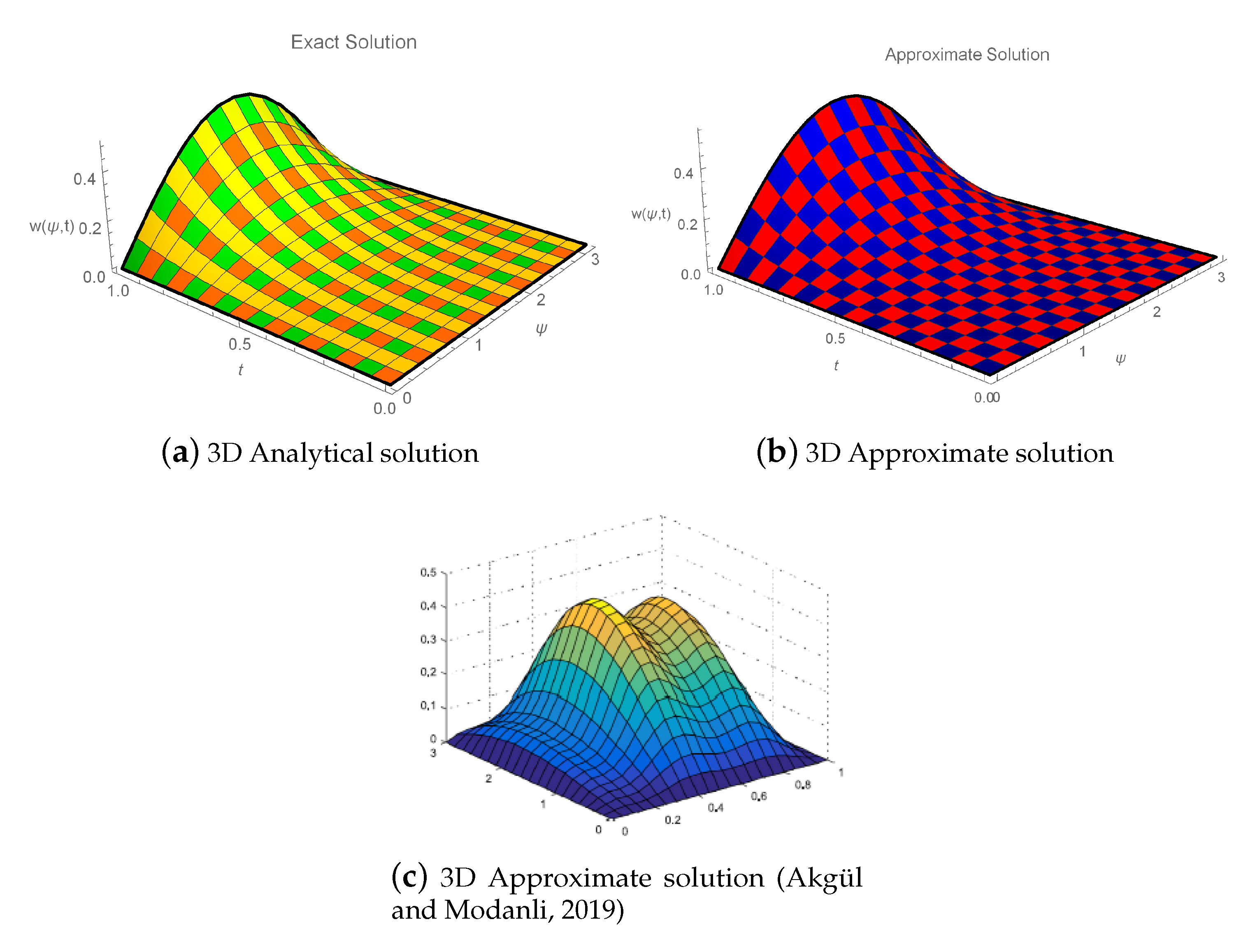
  10. Akgül, A.; Modanli, M. Crank-Nicholson difference method and reproducing kernel function for third order fractional differential equations in the sense of Atangana-Baleanu Caputo derivative. Choas Solitons Fractals 2019, 127, 10–16. [Google Scholar] [CrossRef]
  11. Ashyralyev, A.; Arjmand, D.; Koksal, M. Taylor’s decomposition on four points for solving third-order linear time-varying systems. J. Frankl. Inst. 2009, 346, 651–662. [Google Scholar] [CrossRef]
  12. Khalid, N.; Abbas, M.; Iqbal, M.K.; Baleanu, D. A numerical investigation of Caputo time fractional Allen-Cahn equation using redefined cubic B-spline functions. Adv. Differ. Equ. 2020, 1, 158. [Google Scholar] [CrossRef]
  13. Wu, G.C.; Zeng, D.Q.; Baleanu, D. Fractional impulsive differential equations: Exact solutions, integral equations and short memory case. Fract. Calc. Appl. Anal. 2019, 22, 180–192. [Google Scholar] [CrossRef]
  14. Baleanu, D.; Fernandez, A.; Akgul, A. On a fractional operator combining proportional and classical differintegrals. Mathematics 2020, 8, 360. [Google Scholar] [CrossRef]
  15. Asif, N.A.; Hammouch, Z.; Riaz, M.B.; Bulut, H. Analytical solution of a Maxwell fluid with slip effects in view of the Caputo-Fabrizio derivative. Eur. Phys. J. Plus 2018, 133, 272. [Google Scholar] [CrossRef]
  16. Ghalib, M.M.; Zafar, A.A.; Riaz, M.B.; Hammouch, Z.; Shabir, K. Analytical approach for the steady MHD conjugate viscous fluid flow in a porous medium with nonsingular fractional derivative. Phys. A Stat. Mech. Its Appl. 2020, 554, 123941. [Google Scholar] [CrossRef]
  17. Akram, T.; Abbas, M.; Ismail, A.I.; Ali, N.H.M.; Baleanu, D. Extended cubic B-splines in the numerical solution of time fractional telegraph equation. Adv. Differ. Equ. 2019, 1, 365. [Google Scholar] [CrossRef]
  18. Mohyud-Din, S.T.; Akram, T.; Abbas, M.; Ismail, A.I.; Ali, N.H.M. A fully implicit finite difference scheme based on extended cubic B-spline for fractional advection-diffusion equation. Adv. Differ. Equ. 2018, 1, 109. [Google Scholar] [CrossRef]
  19. Shengjun, H.X.L. An extension of the cubic uniform B-spline curve. J. Comput. Aided Des. Comput. Graph. 2003, 5, 576–578. [Google Scholar]
  20. Abbas, M.; Iqbal, M.K.; Zafar, B.; Zin, S.B.M. New cubic B-spline approximations for solving non-linear third-order Korteweg-de vries equation. Indian J. Sci. Technol. 2019, 12, 1–9. [Google Scholar] [CrossRef]
  21. Fyfe, D. The use of cubic splines in the solution of two-point boundary value problems. Comput. J. 1969, 12, 188–192. [Google Scholar] [CrossRef]
  22. Iqbal, M.K.; Abbas, M.; Wasim, I. New cubic B-spline approximations for solving third-order Emden-Flower type equation. Appl. Math. Comput. 2018, 331, 319–333. [Google Scholar] [CrossRef]
  23. Lang, F.G.; Xu, X.P. A new cubic B-spline method for approximating the solution of a class of non-linear second order boundary value problem with two dependent variables. ScienceAsia 2014, 40, 444–450. [Google Scholar] [CrossRef]
  24. Lin, Y.; Xu, C. Finite difference/spectral approximations for the time-fractional diffusion equation. J. Comput. Phys. 2007, 225, 1533–1552. [Google Scholar] [CrossRef]
  25. Sayevand, K.; Yazdani, A.; Arjang, F. Cubic B-spline collocation method and its applications for anomalous fractional diffusion equations in transport dynamic system. J. Vib. Control 2016, 22, 2173–2186. [Google Scholar] [CrossRef]
Figure 1. Absolute error plot of Example 1 when M ˜ = K = 160 .
Fractalfract 06 00528 g001
Figure 2. Three-dimensional space–time plot of analytical and approximate solutions when γ = 0.37 , M ˜ = K = 80 .
Fractalfract 06 00528 g002
Figure 3. Comparison between 3D analytical, proposed approximate, and approximate [10] solutions of Example 1 for γ = 0.37 and M ˜ = K = 20 .
Fractalfract 06 00528 g003
Figure 4. Comparison between 3D analytical, proposed approximate, and approximate [10] solutions of example 1 for γ = 0.69 and M ˜ = K = 20 .
Fractalfract 06 00528 g004
Figure 5. Comparison between 3D analytical, proposed approximate, and approximate [10] solutions of example 1 for γ = 0.81 and M ˜ = K = 20 .
Fractalfract 06 00528 g005
Figure 6. Absolute error of Example 2 obtained by the proposed scheme when M ˜ = 100 , K = 10 .
Fractalfract 06 00528 g006
Figure 7. Three-dimensional analytic and approximate solutions of Example 2 obtained by the proposed scheme when γ = 0.001 and M ˜ = 100 , K = 10 .
Fractalfract 06 00528 g007
Figure 8. Three-dimensional space–time analytic and approximate solutions of Example 2 obtained by the proposed scheme when γ = 0.001 , M ˜ = K = 80 .
Fractalfract 06 00528 g008
Figure 9. Three-dimensional exact and approximate solutions graphs of Example 2 obtained by the proposed scheme for γ = 0.001 , M ˜ = K = 160 .
Fractalfract 06 00528 g009
Table 1. Maximum error profile for Example 1 when τ = 1 20 and h = π 20 .
( γ , κ ) Proposed SchemeCNFDM [10]
(0.001, 1.44) 0.000105357 0.312670659474578
(0.01, 1.44) 0.000202811 0.316417368682664
(0.37, 0.9) 0.002552621 0.334981685094574
(0.5, 0.529) 0.000015823 0.279273735484124
(0.69, 0.001) 0.007735142 0.162639876741267
(0.81, 0.01) 0.034280707 0.089140237979957
(0.99, 0.001) 0.060474991 0.001420279481709
(0.999, 0.001) 0.061439270 0.002189298564374
Table 2. Absolute error profile for Example 1 when τ = 1 80 and h = π 80 .
( γ , κ ) Proposed SchemeCNFDM [10]
(0.001, 1.33) 0.0000555127 0.482603146665670
(0.01, 1.33) 0.0000263275 0.487508672577419
(0.37, 0.648) 0.0000123132 0.529939808763533
(0.5, 0.280) 0.0000677856 0.460492617848428
(0.69, 0.010) 0.0065096011 0.310451668381897
(0.81, 0.010) 0.0123053210 0.213389947812387
(0.99, 0.001) 0.0176068321 0.089828130903143
(0.999, 0.001) 0.0177875443 0.084419821469902
Table 3. Error analysis for Example 1 when τ = 1 K , h = π M ˜ .
γ κ K = 160 & M ˜ = 160 κ K = 10 & M ˜ = 100
0.001 1.317 3.6850 × 10 6 1.600 0.0007427322
0.01 1.315 5.9170 × 10 7 1.600 0.0005669441
0.37 0.579 4.4978 × 10 6 1.080 0.0001260830
0.5 0.208 1.6306 × 10 6 0.753 0.0000141738
0.69 0.001 3.8884 × 10 3 0.141 0.0000326901
0.81 0.001 6.5879 × 10 3 0.001 0.0375041110
0.99 0.001 9.0213 × 10 3 0.001 0.0963445443
0.999 0.001 9.1037 × 10 3 0.001 0.0986054113
Table 4. The L error norm and order of convergence ρ of Example 1 when M ˜ = 160 .
( γ , κ ) τ L ρ
(0.5, 1.400) 1 4 0.0338561 . . .
(0.5, 0.900) 1 8 0.0066860 2.3402
(0.5, 0.573) 1 16 0.0016284 2.0376
(0.5, 0.432) 1 32 0.0003274 2.3142
Table 5. The L error norm and ρ of Example 1 when K = 160 .
( γ , κ ) h L ρ
(0.5, 0.4348) π 16 0.00252197
(0.5, 0.2580) π 32 0.00058506 2.10789
(0.5, 0.1970) π 64 0.00013258 2.14163
(0.5, 0.2105) π 128 0.00002803 2.24156
Table 6. Absolute error norm for Example 2 when τ = 1 K , h = 1 M ˜ .
γ κ K = 20 & M ˜ = 20 κ K = 80 & M ˜ = 80
0.001 45.911 2.2547 × 10 4 12.500 4.7365 × 10 6
0.01 45.900 2.2537 × 10 4 12.490 2.7841 × 10 6
0.37 45.900 2.1356 × 10 4 12.425 2.6412 × 10 6
0.5 45.900 2.0327 × 10 4 12.393 2.5157 × 10 6
0.69 45.898 1.7814 × 10 4 12.330 1.8088 × 10 6
0.81 45.897 1.5408 × 10 4 12.247 9.8607 × 10 7
0.99 45.897 1.0387 × 10 4 12.127 9.4807 × 10 7
0.999 45.896 1.0092 × 10 4 11.977 2.1244 × 10 7
Table 7. Maximum errors for Example 2 when τ = 1 K , h = 1 M ˜ .
γ κ K = 160 & M ˜ = 160 κ K = 10 & M ˜ = 100
0.001 16.800 2.4679 × 10 6 6.600 5.0317 × 10 5
0.01 16.798 2.3974 × 10 6 6.600 4.6002 × 10 5
0.37 16.735 2.1848 × 10 6 6.533 4.1762 × 10 5
0.5 16.701 1.7302 × 10 6 6.433 2.7052 × 10 5
0.69 16.646 1.7059 × 10 6 6.312 8.9207 × 10 6
0.81 16.595 1.4919 × 10 6 6.275 4.60065 × 10 6
0.99 16.467 8.7779 × 10 7 6.234 2.2419 × 10 6
0.999 16.447 1.6216 × 10 7 6.165 1.87417 × 10 6
Table 8. The L error norm and ρ of Example 2 for M ˜ = 160 .
( γ , κ ) τ L ρ
(0.5, 4.440) 1 4 0.00999346
(0.5, 5.380) 1 8 0.00259925 1.94289
(0.5, 6.600) 1 16 0.00064034 2.02117
(0.5, 8.475) 1 32 0.00015437 2.04902
Table 9. The L errors and ρ of Example 2 when K = 160 .
( γ , κ ) h L ρ
(0.5, 5.00) 1 16 0.00297106
(0.5, 10.50) 1 32 0.00086012 1.78836
(0.5, 14.33) 1 64 0.00024807 1.79378
(0.5, 17.49) 1 128 0.00007100 1.80472
Publisher’s Note: MDPI stays neutral with regard to jurisdictional claims in published maps and institutional affiliations.

