

On the Link between the Langevin Equation and the Coagulation Kernels of Suspended Nanoparticles

Department of Mechanical Engineering, University of Minnesota, Minneapolis, MN 55455, USA
Fractal Fract. 2022, 6(9), 529; https://doi.org/10.3390/fractalfract6090529
Submission received: 7 August 2022
/
Revised: 9 September 2022
/
Accepted: 14 September 2022
/
Published: 18 September 2022
(This article belongs to the Special Issue Advances in Multiparticle Fractal Aggregation)
Abstract
:The ability of the Langevin equation to predict coagulation kernels in the transition regime (ranging from ballistic to diffusive) is not commonly discussed in the literature, and previous numerical works are lacking a theoretical justification. This work contributes to the conversation to gain better understanding on how the trajectories of suspended particles determine their collision frequency. The fundamental link between the Langevin equation and coagulation kernels based on a simple approximation of the former is discussed. The proposed approximation is compared to a fractal model from the literature. In addition, a new, simple expression for determining the coagulation kernels in the transition regime is proposed. The new expression is in good agreement with existing methods such as the flux-matching approach proposed by Fuchs. The new model predicts an asymptotic limit for the kinetics of coagulation in the transition regime.
1. Introduction
Understanding collision-based nano/micrometer-sized particle growth is relevant for predicting pollutant formation, nanoparticle synthesis, powder, and nanotechnology. The latter is important, for example, in the pharmaceutical, mining, cosmetic, and food industries [1,2,3]. Indeed, one of the most important mechanisms of aerosol particle growth is coagulation, whereby particles stick together (aggregation or agglomeration) or experience total coalescence or sintering after collisions [4,5]. In this context, models for particle collision frequencies are needed. Current models are commonly restricted to specific conditions, such as particle interaction forces, flow regime (particle–fluid interaction, either continuum or free molecular), and collision regime (particle–particle interaction, either diffusive or ballistic) [5,6]. However, aerosol coagulation processes commonly take place in the transition regime ranging from ballistic to diffusive. This is a natural consequence of particle growth as larger particles tend to behave more diffusively than smaller ones [7]. However, it has been historically challenging to find expressions for the collision kernels valid for all the regimes due to the lack of theory. In this context, different types of approximate methods can be found in the literature including the flux-matching method [8,9], the Fokker–Planck method [10], interpolation formulas [11,12,13], and the particle trajectory-based method [14]. As stated in Chapter 7 of Fuchs’s book [8], the introduced flux-matching model [8] is a simplification of the problem in which the diffusive flux of particles is assumed to be equivalent to the ballistic flux at the so-called limiting sphere depending on the particle-persistent distance and radii. Although this method has found good agreement with experiments, we can hardly justify that particles may experience such spontaneous transition from diffusive to ballistic motion at the interface of the limiting sphere. Dahneke [9] proposed an approximation of the limiting sphere based on a kinetic description of particle collisions but also relied on the flux-matching assumption. Some authors have suggested solving the Fokker–Planck equation to describe the particle-collision rates, as this equation is expected to be valid in both diffusive and ballistic regimes [10]. However, this equation cannot be solved analytically, and only approximations have been achieved as thoroughly discussed in Refs. [15,16]. A simpler, yet probably effective, approach consists of simulating particle trajectories by solving the Langevin equation and fitting the dimensionless collision kernels for different regimes as done in Refs. [11,12,13]. This method seems to provide us with an accurate estimation of the coagulation kernels; however, they usually do not discuss the limits of the Langevin equation itself, and the fundamental reason why this equation is able to predict collision kernels at different collision regimes seems elusive. Therefore, theoretical methods are needed to fill this gap of knowledge. In this sense, an alternative method was proposed by Gmachowski [14], who derived the collision kernels theoretically from the particles’ trajectories as described by an empirical fractal model introduced by the same author in a previous work [17]. Unfortunately, such a fractal model lacks justification, is an empirical approach, and its relationship with the Langevin equation is not clear. Moreover, to the best of the author’s knowledge, there are no additional works in the literature discussing the particle trajectory-derived collision kernels as proposed by Gmachowski [14]. The trajectories of the particles, either diffusive or ballistic, determine the coagulation kernels because the probability of suspended particle collisions is proportional to their swept volume. In fact, the coagulation kernels in both the ballistic and the diffusive regimes can be obtained from the time derivative of this swept volume when the system of particles is uniform and diluted (vide infra). In addition, the trajectories of Brownian particles may be predicted based on a fractional model [18,19], a fractal model [14], random walks [20], or by solving the Langevin equation with different time steps [21]. The latter is important, as solving the Langevin equation for numerical simulations of aerosol dynamics is currently computationally expensive and the choice of time step may influence the particle collision kernels [21]. Therefore, revealing clearly how the model used for particle trajectory can affect the particle–particle collision frequencies is needed. The most accuratemethod to describe the trajectories of suspended nanoparticles in all the collision regimes is likely the Langevin equation [22]. However, the current solutions of this equation found in the literature are not explicit, making analytical or theoretical works difficult. Consequently, considering the lack of understanding on particle coagulation at different collision regimes and the complexity and/or limited accuracy of the existing approaches, the goals of this work are: (1) to better understand how particle trajectories determine their collision frequency, (2) to explain why the Langevin equation is able to predict collision kernels under different collision regimes, (3) to explore simple approximations for solving the Langevin equation and compare it to fractal models, and (4) to obtain a simple but accurate collision kernel model that may encounter many applications in aerosol transport problems. In this work, the coagulation kernels are analytically obtained based on a new, simple but accurate approximation of the Langevin equation describing the particle’s trajectories. The proposed model predicts the collision kernels of suspended particles in the transition regime. Most importantly, the proposed method shows the ability of the Langevin equation to predict collision kernels at different regimes, and the impact of its parameters is analytically observed in this work as never done before. In addition, the new model predicts a likely universal asymptotic limit for the kinetics of coagulation in the transition regime.
2. Materials and Methods
2.1. The Population Balance Equation
To numerically simulate the evolution of particle size distribution due to interparticle collisions from a macroscopic perspective, the Smoluckowski or population balance equation (PBE) is widely used,
where corresponds to the particle number concentration, the volume of which lies between v and at time t. The left-hand side of this equation represents the time derivative of the particle number concentration. The first integral on the right-hand side is a gain term due to collisions between particles whose combined volumes result in v. Due to the symmetry of this sum, the factor is included to avoid double counting. The second integral represents a loss term due to the collision of particles with volume v with any other particle. How fast particles combine is determined by the collision kernel . It is defined as the number of collisions per unit of time between particles with volumes v and .
2.2. The Collision Kernels
For diluted systems of particles (when interparticle distance is much larger than particle sizes), the diffusive Knudsen number Kn describes the collision regime [12]. Here, corresponds to the particles’ persistent distance, i.e., the average distance travelled by particles before considerably changing direction or relaxing their momentum, and a the particle radius. There are different expressions in the literature for , including Refs. [7,8,9]. The Fuchs expression is preferred here where , and are the particles’ momentum relaxation time ( ratio between the particle’s mass m and its friction coefficient f), and the average Maxwellian velocity (, where is the Boltzmann constant, and T is the surrounding fluid temperature), respectively.
Let us consider a system of many particles and imagine that each particle has a characteristic sphere of radius placed on its center of mass. Then, any collision taking place within this sphere is ballistic. Therefore, as shown in Figure 1 we can distinguish two extreme cases. First, when (or Kn) the particle will experience a diffusive movement, and therefore any collision rate with neighbors will be diffusion-limited. In this regime, particles approach each other with a diffusive trajectory or curvilinear motion (see Figure 1a). Secondly, when (or Kn) the particle will experience a ballistic motion, and collision with neighbors will be ballistically limited. In this regime, particles approach each other with a ballistic trajectory or rectilinear motion (see Figure 1b). However, there is a third case, not represented in this figure, corresponding to the transition between these two extreme regimes. For the aforementioned coagulation regimes, the corresponding collision kernels are explained in the following sections.
2.2.1. Diffusive Regime
When (i.e., Kn), the particles experience a diffusive motion and their relative swept volume can be approximated as a Wiener sausage [23],
where (or ) and (or ) are the particle’s radius and diffusion coefficients, respectively. In addition, t corresponds to the time between collisions. In the limit corresponding to diluted systems, Equation (2) simplifies to
The nanoparticle collision rate in this regime is ,
This equation was originally obtained by Smoluchowski in 1917 by considering a diffusive flux of particles arriving at the surface of another one and neglecting the transient part of the flux that may become important under high particle concentrations. This equation has been recently obtained in a more rigorous way than the Smoluchowski’s approach in Ref. [24].
2.2.2. Ballistic Regime
When (i.e., Kn), the particles’ relative swept volume is directly the product of their cross-section times, their Maxwellian velocity, and both ends of the straight sausage described by the particle motion,
Here, and indicate the average Maxwellian velocity of the i’th and j’th particles, respectively. The corresponding particle collision rate in this regime is ,
This kernel is also derived when considering a flux of particles arriving at the surface of a neighbour as described by the kinetic theory [4].
2.2.3. Transition Regime
The already-introduced diffusive Knudsen number can be generalized to any pair of colliding particles i and j,
As mentioned in the introduction, there is a lack of theory for the transition regime. A practical way of studying it is by introducing a correction function such that,
i.e., is a function allowing us to calculate the coagulation kernel k for all the coagulation regimes by knowing one extreme regime, such as the diffusive one [25]. In the limit , the function and therefore the total collision kernel is diffusive . In the limit , we have where the total collision kernel is ballistic . Table 1 summarizes the different methods found in the literature to calculate the correction function . As explained in the introduction, these methods can be classified into four groups: (1) flux-matching methods [8,9], (2) Fokker–Planck equation-based methods [10], (3) interpolating formulas [11,12,13], and (4) the methods based on particles’ trajectories [14]. The proposed method here belongs to the latter group where the function is derived from the Langevin equation. This is explained in the following section.
2.3. Langevin Dynamics
The trajectory followed by an aerosol particle can be accurately described based on the Langevin equation [22],
It is a linear, first-order, inhomogeneous stochastic differential equation corresponding to Newton’s conservation of linear momentum for a single aerosol particle. The main assumption of this model is that external forces caused by the surrounding fluid can be split into a systematic part (i.e., , corresponding to the drag force) and a stochastic part (i.e., , or the Brownian force). The Brownian force is typically justified as the result of stochastic collisions of the particle and the fluid molecules. However, as pointed out by Pomeau and Piasecki [26], if the fluid molecules are modeled as hard spheres then both the friction and the Brownian forces are due to particle–fluid molecule collisions. The same authors proposed that on average and at equilibrium the particle velocity fluctuations predicted by the Langevin equation are symmetrical in time. In addition, the dependence on the fluid viscosity shows that the random force is due to the fluctuations of the fluid around the suspended particle, which is a consequence of the discrete or molecular nature of the fluid. The term stands for the net external forces such as electric, magnetic, and interparticle forces not considered in the present work. The Brownian stochastic force has the following properties,
where is the Dirac function. This means that the Brownian force is uncorrelated in time and can be mathematically modeled as a Gaussian noise with moments given by Equations (10a) and (10b). The Langevin equation is based on the idea that particle–fluid molecular collisions have a much shorter characteristic time than the particle momentum relaxation time, and this may be valid regardless of the particle’s size (in the nano- to micrometer range), the fluid temperature, and pressure. Based on the fluctuation–dissipation theorem, we conclude that the Langevin equation is limited to a thermally equilibrated particle–fluid system. Otherwise, Equation (10b) is no longer valid [27]. For additional discussions on the limitations of the Langevin equation, the reader is referred to [26,27].
Uhlenbeck and Ornstein [28] obtained the following analytical solution for the particle average mean squared displacement ,
The following asymptotic limits of Equation (11) can be verified. At , we obtain where is the root mean squared Maxwellian velocity, meaning that particle movement is ballistic at short time scales. On the other hand, at we obtain , which is the classical mean squared displacement predicted by Einstein’s theory of Brownian motion in a three-dimensional system, meaning that particle movement becomes diffusive for long times. However, this analytical expression is not explicit, making its application difficult for theoretical analysis; therefore, an approximation for this expression is proposed in the following section.
2.4. Approximating Langevin Dynamics
An approximation for Equation (11) was proposed by Gmachowski [14] based the following fractal model,
where . This fractal model is based on the idea that in the limit the particle moves ballistically, and its trajectory can be described as a fractal object with a fractal dimension close to 1. Moreover, in the limit the particle moves diffusively, and its trajectory corresponds to a random walk and exhibits a fractal dimension of 2. The reader is referred to [17] for additional details on this model. In addition, it is worth mentioning that previous works have explored a generalization of Brownian dynamics based on fractional Brownian motion [29,30], and on a fractional Langevin model [18,19]. Fractional Brownian motion allows for lifting the property of time uncorrelation in the Brownian force as described in Equation (10b) and therefore offers a more general framework to study Brownian motion. Taking time correlation into account may be important to study aerosol dynamics when the time between consecutive collisions is too short for the particle to reach thermal equilibrium with the surrounding fluid, which is the case at high particle concentrations [31], or when particles are diluted but the turbulence of the fluid induces correlation in time [32]. Moreover, an alternative approximation of this trajectory is to use random walks in which the length of the walk path may be taken to the persistent distance; however, a different persistent distance than the one used in this work has to be introduced to accurately approximate the Langevin equation as discussed in Ref. [20]. In this work, an alternative approach is proposed based on the following explicit equation (see Appendix A for additional details):
Equation (13) has similar asymptotic limits as Equation (11), i.e., at Equation (13) leads to where is the average Maxwellian velocity, meaning that particle movement is ballistic at short times. On the limit , Equation (13) leads to , meaning that particle movement becomes diffusive at long times. The MSD predicted by Equation (13) as compared to Equation (11) obtained by [28] is shown in Figure 2 as a function of the dimensionless time. The MSD is normalized by the Fuchs persistent distance , and time is normalized by the momentum relaxation time . In the range of time considered here (from to ), the proposed model shows a maximum error of 10% as compared to Uhlenbeck and Ornstein’s equation [28]. In addition, the fractal model given by Equation (12) exhibits an increasing error that goes up to 38% in the studied range. Note that fitting the fractal model to find the best h to be in agreement with the method proposed in this work gives the value , which is larger than the proposed by [14] and still exhibits difficulty in describing the MSD for times . This means that approximating the Langevin equation based on a fractal model based on a single fractal dimension has limited accuracy.
3. Results
3.1. Derivation of the Coagulation Kernel
Following the approach of Gmachowski [14] and considering that particles’ relative swept volume can be described by Equations (3) and (5) for the diffusive and ballistic regimes, respectively, we can reach our conclusion. In addition, considering that particles MSD are and in the diffusive and ballistic regimes, respectively, the coagulation kernels can be rewritten as,
Having Equations (2) and (5) in mind, then Equations (14a) and (14b) are interpreted as the time derivative of the particles’ swept volume defined by their mean squared trajectories. Moreover, in the transition regime we may expect , which is valid when the mean squared displacements and particles’ radii are related according to the following equation,
where the mean squared displacements and can be expressed in terms of the proposed approximation of Langevin dynamics given by Equation (13):
In the case of monodisperse particles, this expression is reduced to
where the approaching time t for two colliding particles is direcly obtained:
The collision kernel in the transition regime can be expresed as follows,
where t is the approaching time for two colliding particles based on Equation (17). Based on Equation (15), we arrive at the proposed coagulation kernel approximation
Finally, it can be expressed in terms of the diffusive Knudsen number based on the Fuchs persistent distance :
3.2. Proposed Coagulation Kernels
Based on the expressions derived in the previous section, the proposed transition regime correction for the coagulation kernel is
In Figure 3, the proposed kernel corrective function, given by Equation (20), is compared with other methods found in the literature. In both extreme regimes, i.e., ballistic (Kn) and diffusive (Kn), the agreement with the literature is excellent which shows the ability of the Langevin equation to predict both extreme regimes. This can be mathematically checked by evaluating both limits in Equation (20). Moreover, in the transition regime, the agreement is very good in the near-ballistic regime (when Kn). However, the proposed method seems to attain the diffusive regime (as Kn decreases) much more quickly than the methods proposed in the literature; that is, the correction function is larger than the values proposed in the literature for the near-diffusive regime (when Kn). Overall, as discussed later, the error is still less than 18% regarding the interpolation equations from Refs. [8,12,13]. It is interesting to note that the improvements in the accuracy of predicting particle trajectories introduced in this work have more important consequences on collision kernels in the near-ballistic regime. Indeed, some sensitivity analysis on the parameter of Equation (13) shows a direct impact on the ballistic and near-ballistic regime. Moreover, replacing this value by 1 as we may obtain based on the approximation of the Langevin equation proposed by Trzeciak [33], results in an overestimation of the collision kernels in the ballistic limit. This is explained by the fact that Equation (14b) relies on an approximation of the mean squared displacement. It is also interesting to note that, as observed in Figure 3, the kernel based on the fractal model proposed by Gmachowski [14] gives exactly the same result as the harmonic mean method which is derived in Appendix B. In addition, as discussed by Trzeciak [33], the harmonic mean collision kernel can be derived from the flux-matching approach developed by Fuchs when the size of the limiting sphere is collapsed to the physical size of particles.
In this context, a natural question is about the role played by the Cunningham correction factor and what is the maximum Kn up to which the diffusive kernel (corrected by the Cunningham factor) is still accurate when the change in coagulation regime is induced by a change in the flow regime (from continuum to free molecular). Figure 4a compares the proposed coagulation kernel calculated from Equations (8) and (20) with the literature and the asymptotic values, namely ballistic given by Equation (6) and diffusive given by Equation (4). In the latter, the diffusion coefficient is determined as where is the friction coefficient, is the surrounding gas viscosity, and is the Cunningham slip correction factor [34],
where Kn is the classical gas Knudsen number, consisting of the ratio between the gas mean free path and the particle’s radius a. When Kn, the particle is in the continuum flow regime and the friction coefficient is given by the Stokes relation (); however, when Kn, the particle is in the free molecular flow regime and the friction coefficient is given by the Epstein relation (). For spherical particles, the Cunningham slip factor allows for simulation of the transition between both flow regimes. To study this dependency, the coagulation kernels based on Equation (8) and the correction functions (presented in Table 1) are determined. The results are presented in Figure 4, where the surrounding gas is air at a constant temperature of 1700 K and pressure of kPa. The mass density of the particles is g/cm, and diameters range from 1 nm to 1000 m.
In Figure 4a, the different coagulation kernels are compared with the diffusive one corrected by the Cunningham slip factor (dashed line). In addition, the ballistic kernel (dash-dotted line) is included to clearly show the change of regime. In this figure, we observe that the proposed method stays closer to the diffusive kernel (corrected by the Cunningham slip factor) up to larger values of Kn than other methods from the literature. However, the proposed equation never goes beyond these limits, and the difficulty of accurately predicting the transition regime seems to be related to the different assumptions made on the derivation of the new function.
Figure 4b represents the relative variation of the coagulation kernels (from the present work and others from the literature) with proposed by [12]. The latter is considered as the reference because it comes from Langevin simulations and was found to be in good agreement with both numerical and experimental works [7,13]. As observed here, the proposed method overestimates in a maximum of 18% of the referenced one (i.e., ) when Kn. Remarkably, Gmachowski [14] or, equivalently, the harmonic mean methods, deviate in almost the same order of magnitude. However, both methods systematically underestimate the coagulation kernel. In this context, the simplicity of the proposed method in comparison with those found in the literature is highlighted.
4. Discussion
4.1. Comparison with Experiments
The classical method introduced by Fuchs [8], although it is found to be in very good agreement with more recent works, has not been exempt of criticism, especially in the near-diffusive regime. Davies [35] reviewed the experimentally measured coagulation kernels of eight articles and concluded that Fuchs’ [8] interpolation method can underestimate the real coagulation kernels in the near-diffusive regime. Subsequently, Lee and Chen [36] suggested that this difference with experimental data may be explained by particles’ polydispersity. The results of Kim et al. [37] show a slightly larger collision kernels than those predicted by Fuchs [8] and Dahneke [9]. Additionally, Kerker et al. [38] obtained slightly smaller kernels than Fuchs [8] in the same regime. Despite these sources of uncertainties, the Fuchs [8] method is widely accepted [12]. Indeed, in the following section, the practical effects of using one of the aforementioned methods for the coagulation kernels in the transition regime are discussed.
4.2. The Effect on the PSD and the Kinetics of Coagulation
An important question that naturally arises here is What are the practical effects on the particle size distribution (PSD) and also the kinetics of coagulation when selecting one of the previously mentioned methods to evaluate the coagulation kernels? To answer this question, a new version of the NGDE code, originally developed by Prakash et al. [39] is developed (see Appendix C). In this context, the PBE (1) is discretized into nodes as
where two particles of volumes and collide with frequency to form a third one of volume . To take into account that this volume may fall between two consecutive nodes i.e. and (or and ), the size-splitting operator is used:
Different methods by which to evaluate the coagulation kernels in Equation (22) are evaluated, studying the transition regime without considering nucleation or surface growth. Only in references [12] and [14] is the harmonic mean discussed, and the proposed methods are considered to be representative of the four groups of methods discussed before. A total of nodes for discretizing the PSD, and the same thermodynamic and particle properties used in the previous section are considered here. In addition, the initial number concentration was adapted for each case to simulate a constant particle volume fraction of %. In this case, the corrections for high volume fraction are negligible [31,40,41,42]. Moreover, Equation (22) is solved based on a forward Euler method with time step , where is a constant value, is the minimum collision kernel among all pairs of particles () in the system, and is the total particle number concentration at time t. In these simulations, the collision kernels are determined by combining Equations (4), (7), (8) and (20).
Figure 5a–c presents the time-evolving, volume-based geometric mean and geometric standard deviation as a function of time (bottom horizontal axis) and as a function of the diffusive Knudsen number Kn (top horizontal axis). Different coagulation regimes, namely Kn (near ballistic), Kn (intermediate), and Kn (near diffusive) are simulated. Here, Kn stands for the initial diffusive Knudsen number. These diffusive Knudsen numbers are calculated based on the volume equivalent mean diameter. Both and values are calculated as described in Appendix D. In all simulations, as time evolves, the particles grow due to stochastic collisions with neighbors. Note that the diffusive Knudsen number is always smaller at the end of the simulation compared to the beginning as larger particles experience a more diffusive motion [7,43]. Geometric mean volume equivalent diameters are always increasing in time due to coagulation, and only a small difference is found between the different methods. The geometric values are increasing from the initial monodisperse particles () reaching asymptotic values between and corresponding to the diffusive and ballistic limits, respectively. The increase in polydispersity in time is a natural consequence of coagulation, and is larger in the ballistic regime due to the size dependence of the coagulation kernel, which is not found in the diffusive regime. These simulations are in good agreement with the limits for the corresponding diffusive and ballistic self-preserving size distribution regime found in the literature [25,44].
In Figure 6a–c, the particle number concentrations as a function of time are presented. For all the cases studied here, the PSD is not considerably affected by the particular method used for coagulation kernels determination. When analyzing individual PSD (not shown here), a very good agreement is observed for larger particle volumes, and only a minor difference is reached for smaller particle volumes. However, focusing on the total number concentration is a simplified and too macroscopic a view of the problem. A more relevant effect is observed in terms of the kinetics of coagulation, which is discussed in more detail as follows.
4.3. The Asymptotic Size Distribution and Collision Kinetics
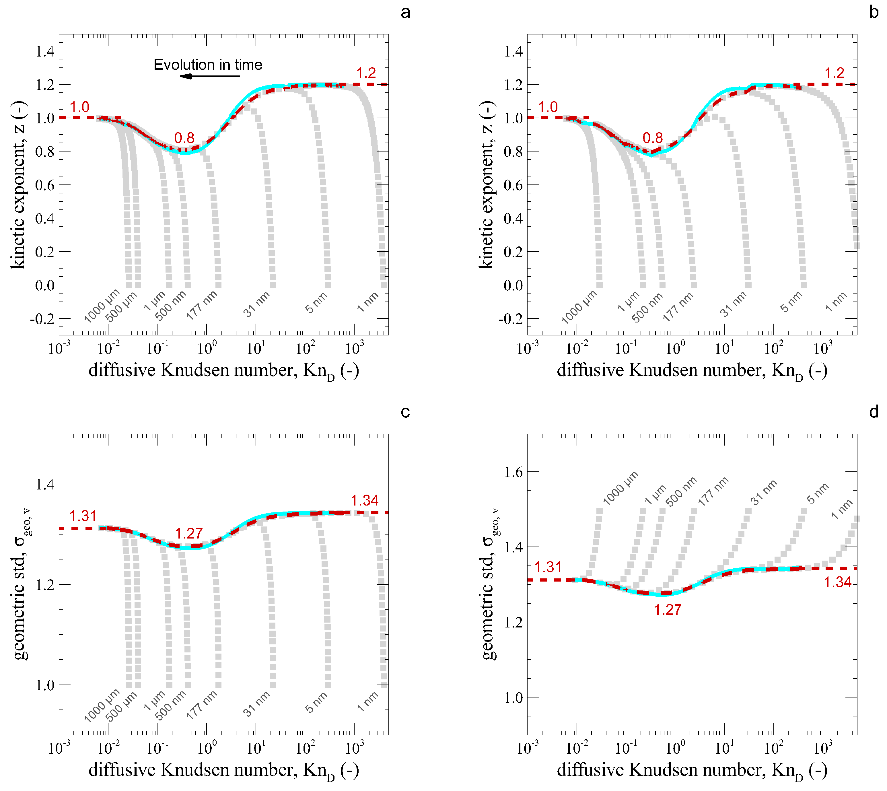
As observed in the previous section, the proposed method seems accurate in simulating the coagulation process. However, a systematic analysis is needed to show its ability to predict the asymptotic limit of particle coagulation, where is the characteristic time of collisions based on the initial average collision kernel and the initial particle number concentration . The kinetic exponents z, calculated as the exponent of the power law , where is the total particle number concentration at time t is studied. This is done for a set of simulations of spherical particle coagulation with initially monodisperse (Figure 7a) and polydiserse (Figure 7b) size distribution under the same thermodynamic conditions and particle diameters as presented in previous sections. These particle diameters are indicated for each individual simulation in Figure 7. All simulations start at values , which are reported to enlighten how the asymptotic values are reached regardless of the initial condition. As highlighted by the red-dashed line, all simulations nicely converge to an asymptotic limit that may be linked to a self-preserving size-distribution regime. This is a remarkable observation suggesting that the kinetics of coagulation may be universal in the asymptotic limit . Note that previous works [7,45,46,47] have only revealed isolated kinetic exponents of the asymptotic ballistic , transition , and a diffusive regime of initially monodisperse particles. However, they have not revealed the whole asymptotic curve as shown here. In addition, previous works have not observed that even when the initial size distribution is polydisperse the system still attains the same asymptotic z function. Observing the asymptotic z curve, we note that coagulation is faster (z is higher) in the ballistic limit. Indeed, smaller particles, despite having a lower collision cross section, move much faster than larger ones, and this results in higher collision rates with neighbors (see Figure 4). Moreover, the kinetics are slower in the transition regime due to the more prominent role of particle friction due to the lower Cunningham correction factor overcoming the increase in collision rate that we may expect as the particles are larger in size. This Cunningham factor reaches an asymptotic value for larger particle sizes, explaining why the symptotic z is constant for diffusive Knudsen numbers ≤10. In addition, for all the studied conditions and for all collision regimes, the proposed model shows a maximum error of ∼3% on the kinetic exponent as compared to the reference method [12] (see Figure S1 in the Supplementary Materials). This maximum deviation is observed in the near-ballistic regime and a negligible error is observed in both the ballistic and the diffusive limits.
On the other hand, as shown in Figure 7c,d, the asymptotic are observed for particle collisions over the entire range of diffusive Knudsen numbers ranging from diffusive to ballistic. To accurately predict , the number of nodes in the NGDE code is increased to . The long time asymptotic limit of has been previously observed by different authors for initially monodisperse particles [5,48] where was observed in the diffusive, in the transition, and in the ballistic regime. Notably, the same asymptotic values are also observed when the initial particle size distribution is considered lognormal with . Intriguingly, as opposed to the case of initial monodisperse particles, the in this case is decreasing in time to reach the asymptotic self-preserving values mentioned above. This is found to be consistent for particles over the whole range of diffusive Knudsen numbers. These values are in excellent agreement with current simulations. In Figure 7, the continuous cyan line is the asymptotic curve retrieved based on the proposed approach. The proposed model shows a maximum error of % on the as compared to the reference method [12] (see Figure S2 in the Supplementary Materials). This maximum deviation is observed in the near-ballistic regime and a negligible error is observed in both the ballistic and the diffusive regimes.
5. Conclusions
From this work, the following conclusions are drawn.
- As theoretically shown in this work, the accuracy involved in solving the Langevin equation has a direct impact on modeling the suspended particles’ collision frequency.
- A new and accurate approximation of the mean squared displacement of the Langevin equation in the absence of external forces is proposed. This is an explicit equation that may be used for future theoretical works involving the Langevin equation.
- The new approximation of the Langevin equation allows us to obtain a new equation to predict the collision kernels in the transition regime. This new equation is simple and accurate. For example, it shows less than a 3% error in predicting the coagulation kinetics and less than a 1% error in predicting the particle size distribution along different regimes. It may be used for different applications involving aerosol transport processes such as coagulation and condensation.
- This work brings us additional understanding on the properties of the Langevin equation that have a direct impact on predicting collision kernels. Despite different works in the literature have derived collision frequencies based on Langevin dynamics simulations, discussing the hability of the Langevin equation to predict this phenomena from a theoretical perspective is rarely seen. To the best of the author’s knowledge, there are no previous works deriving the collision kernels theoretically from the Langevin equation, as is the case here.
- The proposed model predicts a likely universal asymptotic kinetics of coagulation in the limit independent of the initial condition (e.g., different particle size or polydispersity). It is suggested that such a limit is due to the self-preserving size distribution as found to be correlated with the asymptotic polydispersity limit. This supports the idea that the physics of coagulation in the diluted regime is well parametrized by the diffusive Knudsen number. It also means that coagulation reaches an asymptotic limit in time with predictable consequences not only for the size distribution but also for the coagulation kinetics.
- The analysis presented in this work may be applied to theoretically study the accuracy of discrete element methods to predict coagulation kernels whether they solve the Langevin equation explicitly [49] or based on Monte Carlo methods [7]. Moreover, this work shows the importance of an accurate solution of the Langevin equation to predict collision kernels successfully. This is significant for choosing a time step in numerical simulations of aerosol dynamics [21].
Supplementary Materials
The following supporting information can be downloaded at: https://www.mdpi.com/article/10.3390/fractalfract6090529/s1, Figure S1: The relative error calculated as where and are the geometric standard deviation determined by our, and the reference method, respectively. They are determined for initially monodisperse (a) and polydisperse (b) spherical particles. Figure S2: The relative error calculated as where and are the kinetic exponents determined by our, and the reference method, respectively. They are determined for initially monodisperse (a) and polydisperse (b) spherical particles.
Funding
This research received no external funding.
Data Availability Statement
Not applicable.
Acknowledgments
Thanks are due to Jérôme Yon, Francisco Cepeda and Alejandro Jerez for their re-reading of an earlier version of this manuscript and their insightful comments.
Conflicts of Interest
The author declares no conflict of interest.
Abbreviations
The following abbreviations are used in this manuscript:
| MSD | Mean squared displacement |
| PBE | Population Blance Equation |
| PSD | Particle Size Distribution |
| NGDE | Nodal General Dynamics Equation solver |
| SM | Supporting Material |
Appendix A. Derivation of Equation (13)
When we try to obtain the dimensionless time from Equation (11) derived by [28] we arrive to,
where W corresponds to the Lambert, Omega or product logarithm function defined as the inverse of the function . Trzeciak [33] proposed to approximate it to obtain,
however, as we show in the present work, better agreement with Langevin Dynamics is found based on the following equation,
where , which is close to the previous expression but not equivalent.
Appendix B. Derivation of the Harmonic Mean Collision Kernel Approximation
The Harmonic mean method simply suggests to approximate the collision kernel in the transition regime as the harmonic mean of thos in the ballistic and diffusive,
Therefore, the corresponding transition regime correction function is,
where, for monodisperse particle collisions we have and then replacing in Equation (A5) leads to,
Then considering the diffusive Knudsen number we finally obtain,
Appendix C. Population Balance Code
Population balance simulations have been conducted by using a developed C++ code, which is available under the following Git repository https://gitlab.com/jmoranc1/ngde_cpp.git.
Appendix D. Volume-Based Geometric Mean and Standard Deviation
References
- Meierhofer, F.; Fritsching, U. Synthesis of Metal Oxide Nanoparticles in Flame Sprays: Review on Process Technology, Modeling, and Diagnostics. Energy Fuels 2021, 35, 5495–5537. [Google Scholar] [CrossRef]
- Muzzio, F.J.; Shinbrot, T.; Glasser, B.J. Powder Technology in the Pharmaceutical Industry: The Need to Catch up Fast. Powder Technol. 2002, 124, 1–7. [Google Scholar] [CrossRef]
- van Ommen, J.R.; Valverde, J.M.; Pfeffer, R. Fluidization of nanopowders: A review. J. Nanopart. Res. 2012, 14, 737. [Google Scholar] [CrossRef] [PubMed]
- Friedlander, S.K. Smoke, Dust, and Haze; Oxford University Press: New York, NY, USA, 2000; Volume 198. [Google Scholar]
- Eggersdorfer, M.L.; Pratsinis, S.E. Agglomerates and aggregates of nanoparticles made in the gas phase. Adv. Powder Technol. 2014, 25, 71–90. [Google Scholar] [CrossRef]
- Jeldres, R.I.; Fawell, P.D.; Florio, B.J. Population balance modelling to describe the particle aggregation process: A review. Powder Technol. 2018, 326, 190–207. [Google Scholar] [CrossRef]
- Morán, J.; Yon, J.; Poux, A.; Corbin, F.; Ouf, F.X.; Siméon, A. Monte Carlo Aggregation Code (MCAC) Part 2: Application to soot agglomeration, highlighting the importance of primary particles. J. Colloid Int. Sci. 2020, 575, 274–285. [Google Scholar] [CrossRef]
- Fuchs, N.A. The Mechanics of Aerosols; Pergamon Press: Oxford, UK, 1964. [Google Scholar]
- Dahneke, B. Simple kinetic theory of Brownian diffusion in vapors and aerosols. In Theory of Dispersed Multiphase Flow; Academic Press: Cambridge, MA, USA, 1983; pp. 97–133. [Google Scholar] [CrossRef]
- Sahni, D. An exact solution of fokker-planck equation and brownian coagulation in the transition regime. J. Colloid Int. Sci. 1983, 91, 418–429. [Google Scholar] [CrossRef]
- Azarov, I.; Veshchunov, M. Development of the new approach to the Brownian coagulation theory: Transition regime. J. Eng. Phys. Thermophys. 2010, 19, 128–137. [Google Scholar] [CrossRef]
- Gopalakrishnan, R.; Hogan, C.J., Jr. Determination of the transition regime collision kernel from mean first passage times. Aerosol Sci. Technol. 2011, 45, 1499–1509. [Google Scholar] [CrossRef]
- Polovnikov, P.; Azarov, I.; Veshchunov, M. Advancement of the kinetic approach to Brownian coagulation on the base of the Langevin theory. J. Aerosol Sci. 2016, 96, 14–23. [Google Scholar] [CrossRef]
- Gmachowski, L. The aerosol particle collision kernel considering the fractal model of particle motion. J. Aerosol Sci. 2013, 59, 47–56. [Google Scholar] [CrossRef]
- Kumar, V.; Menon, S.G. Condensation rate on a black sphere via Fokker-Planck equation. J. Chem. Phys. 1985, 82, 917–920. [Google Scholar] [CrossRef]
- de Monvel-Berthier, A.B.; Dita, P. Brownian motion near an absorbing sphere. J. Stat. Phys. 1991, 62, 729–736. [Google Scholar] [CrossRef]
- Gmachowski, L. Fractal model of the transition from ballistic to diffusive motion of a Brownian particle. J. Aerosol Sci. 2013, 57, 194–198. [Google Scholar] [CrossRef]
- Deng, W.; Barkai, E. Ergodic properties of fractional Brownian-Langevin motion. Phys. Rev. E 2009, 79, 011112. [Google Scholar] [CrossRef]
- Lutz, E. Fractional langevin equation. In Fractional Dynamics: Recent Advances; World Scientific: Singapore, 2012; pp. 285–305. [Google Scholar] [CrossRef]
- Morán, J.; Yon, J.; Poux, A. Monte carlo aggregation code (MCAC) Part 1: Fundamentals. J. Colloid Int. Sci. 2020, 569, 184–194. [Google Scholar] [CrossRef]
- Henry, C.; Minier, J.P.; Mohaupt, M.; Profeta, C.; Pozorski, J.; Tanière, A. A stochastic approach for the simulation of collisions between colloidal particles at large time steps. Int. J. Multiph. Flow 2014, 61, 94–107. [Google Scholar] [CrossRef]
- Langevin, P. Sur la théorie du mouvement brownien. Compt. Rendus 1908, 146, 530–533. [Google Scholar] [CrossRef]
- Berezhkovskii, A.; Makhnovskii, Y.A.; Suris, R. Wiener sausage volume moments. J. Stat. Phys. 1989, 57, 333–346. [Google Scholar] [CrossRef]
- Veshchunov, M. A new approach to the Brownian coagulation theory. J. Aerosol Sci. 2010, 41, 895–910. [Google Scholar] [CrossRef]
- Otto, E.; Fissan, H.; Park, S.; Lee, K. The log-normal size distribution theory of Brownian aerosol coagulation for the entire particle size range: Part II—Analytical solution using Dahneke’s coagulation kernel. J. Aerosol Sci. 1999, 30, 17–34. [Google Scholar] [CrossRef]
- Pomeau, Y.; Piasecki, J. The Langevin equation. C R Phys. 2017, 18, 570–582. [Google Scholar] [CrossRef]
- Zwanzig, R. Nonequilibrium Statistical Mechanics; Oxford University Press: Oxford, UK, 2001. [Google Scholar]
- Uhlenbeck, G.E.; Ornstein, L.S. On the theory of the Brownian motion. Phys. Rev. 1930, 36, 823. [Google Scholar] [CrossRef]
- Hairer, M.; Li, X.M. Averaging dynamics driven by fractional Brownian motion. Ann. Probab. 2020, 48, 1826–1860. [Google Scholar] [CrossRef]
- Hairer, M.; Li, X.M. Generating diffusions with fractional Brownian motion. Commun. Math. Phys. 2022, 1–51. [Google Scholar] [CrossRef]
- Trzeciak, T.M.; Podgórski, A.; Marijnissen, J.C. Brownian coagulation in dense systems: Thermal non-equilibrium effects. J. Aerosol Sci. 2014, 69, 1–12. [Google Scholar] [CrossRef]
- Bec, J.; Ray, S.S.; Saw, E.W.; Homann, H. Abrupt growth of large aggregates by correlated coalescences in turbulent flow. Phys. Rev. E 2016, 93, 031102. [Google Scholar] [CrossRef]
- Trzeciak, T.M. Brownian Coagulation at High Particle Concentrations. Ph.D. Thesis, Delft University of Technology, Delft, The Netherlands, 2012. [Google Scholar]
- Sorensen, C.; Wang, G. Note on the correction for diffusion and drag in the slip regime. Aerosol Sci. Technol. 2000, 33, 353–356. [Google Scholar] [CrossRef]
- Davies, C. Coagulation of aerosols by Brownian motion. J. Aerosol Sci. 1979, 10, 151–161. [Google Scholar] [CrossRef]
- Lee, K.; Chen, H. Coagulation rate of polydisperse particles. Aerosol Sci. Technol. 1984, 3, 327–334. [Google Scholar] [CrossRef]
- Kim, D.; Park, S.; Song, Y.; Kim, D.; Lee, K. Brownian coagulation of polydisperse aerosols in the transition regime. J. Aerosol Sci. 2003, 34, 859–868. [Google Scholar] [CrossRef]
- Kerker, M.; Chatterjee, A.; Cooke, D. Brownian coagulation of aerosols in the transition regime. Pure Appl. Chem. 1976, 48, 457–462. [Google Scholar] [CrossRef]
- Prakash, A.; Bapat, A.; Zachariah, M. A simple numerical algorithm and software for solution of nucleation, surface growth, and coagulation problems. Aerosol Sci. Technol. 2003, 37, 892–898. [Google Scholar] [CrossRef]
- Heine, M.; Pratsinis, S.E. Brownian coagulation at high concentration. Langmuir 2007, 23, 9882–9890. [Google Scholar] [CrossRef] [PubMed]
- Buesser, B.; Heine, M.; Pratsinis, S.E. Coagulation of highly concentrated aerosols. J. Aerosol Sci. 2009, 40, 89–100. [Google Scholar] [CrossRef]
- Veshchunov, M.; Tarasov, V. Extension of the Smoluchowski theory to transitions from dilute to dense regime of Brownian coagulation: Triple collisions. Aerosol Sci. Technol. 2014, 48, 813–821. [Google Scholar] [CrossRef]
- Thajudeen, T.; Deshmukh, S.; Hogan, C.J., Jr. Langevin simulation of aggregate formation in the transition regime. Aerosol Sci. Technol. 2015, 49, 115–125. [Google Scholar] [CrossRef]
- Vemury, S.; Kusters, K.A.; Pratsinis, S.E. Time-lag for attainment of the self-preserving particle size distribution by coagulation. J. Colloid Int. Sci. 1994, 165, 53–59. [Google Scholar] [CrossRef]
- Pierce, F.; Sorensen, C.; Chakrabarti, A. Computer simulation of diffusion-limited cluster-cluster aggregation with an Epstein drag force. Phys. Rev. E 2006, 74, 021411. [Google Scholar] [CrossRef]
- Mountain, R.D.; Mulholland, G.W.; Baum, H. Simulation of aerosol agglomeration in the free molecular and continuum flow regimes. J. Colloid Int. Sci. 1986, 114, 67–81. [Google Scholar] [CrossRef]
- Heinson, W.; Sorensen, C.; Chakrabarti, A. Computer simulation of aggregation with consecutive coalescence and non-Coalescence stages in Aerosols. Aerosol Sci. Technol. 2010, 44, 380–387. [Google Scholar] [CrossRef]
- Goudeli, E.; Eggersdorfer, M.L.; Pratsinis, S.E. Coagulation–Agglomeration of fractal-like particles: Structure and self-preserving size distribution. Langmuir 2015, 31, 1320–1327. [Google Scholar] [CrossRef] [PubMed]
- Isella, L.; Drossinos, Y. Langevin agglomeration of nanoparticles interacting via a central potential. Phys. Rev. E 2010, 82, 011404. [Google Scholar] [CrossRef] [PubMed]
Figure 1.
The particle-persistent distance and the particle’s radius a are shown. The corresponding diffusive Knudsen numbers Kn are indicated along with the trajectories of colliding monodisperse particles in the (a) diffusive and (b) ballistic coagulation regimes.
Figure 1.
The particle-persistent distance and the particle’s radius a are shown. The corresponding diffusive Knudsen numbers Kn are indicated along with the trajectories of colliding monodisperse particles in the (a) diffusive and (b) ballistic coagulation regimes.

Figure 2.
Approximation of the normalized mean squared displacement (MSD) normalized by the squared Fuch’s persistent distance as a function of the dimensionless time where is the momentum relaxation time. The proposed method given by Equation (13) is compared with [28] given by Equation (11) and the fractal model proposed by [14].
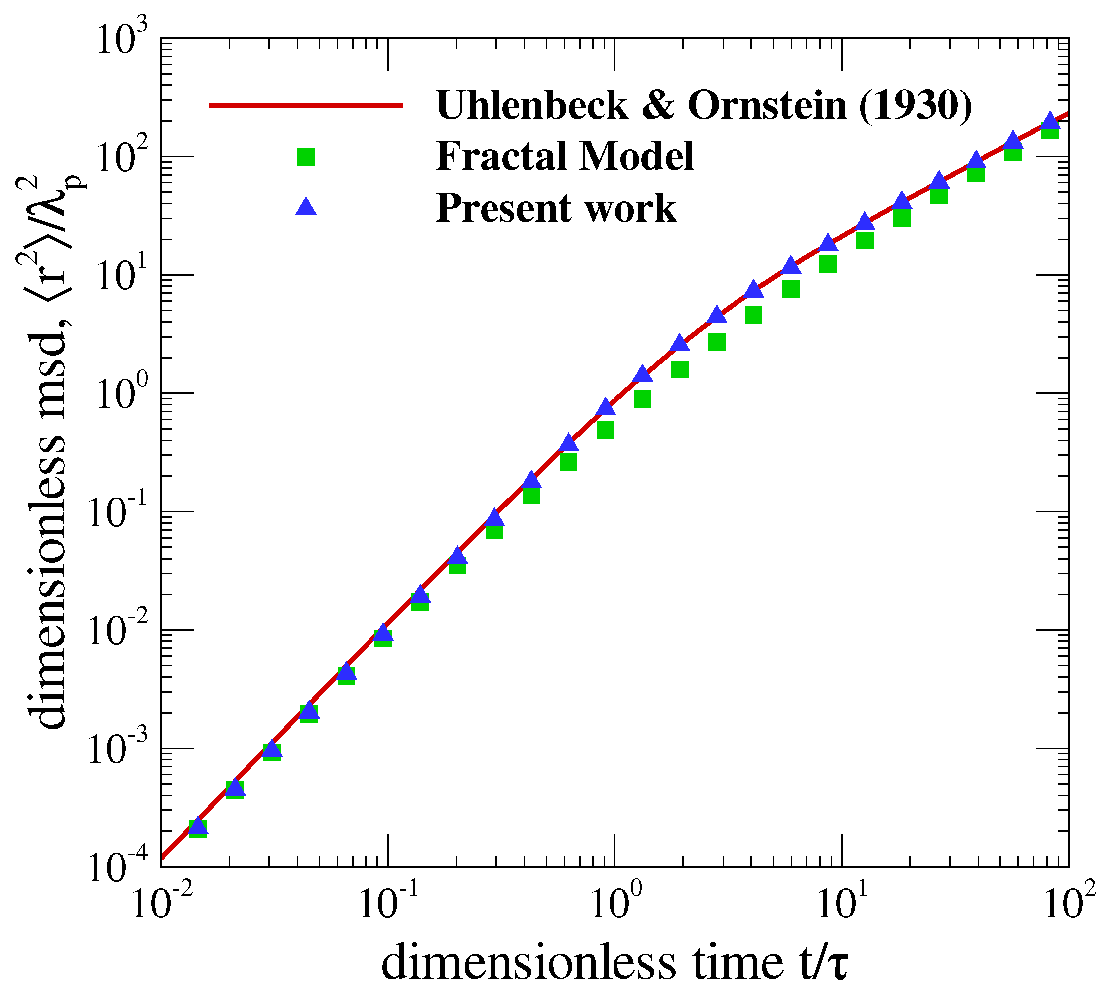
Figure 3.
Coagulation kernel correction function as a function of the diffusive Knudsen number . The proposed model, given by Equation (20) is compared with the literature. Fuchs (1989) [8], Dahneke (1983) [9], Sahni (1983) [10], Gopalakrishnan et al. (2011) [12], Polovnikov et al. (2016) [13], Gmachowski (2013a) [14].
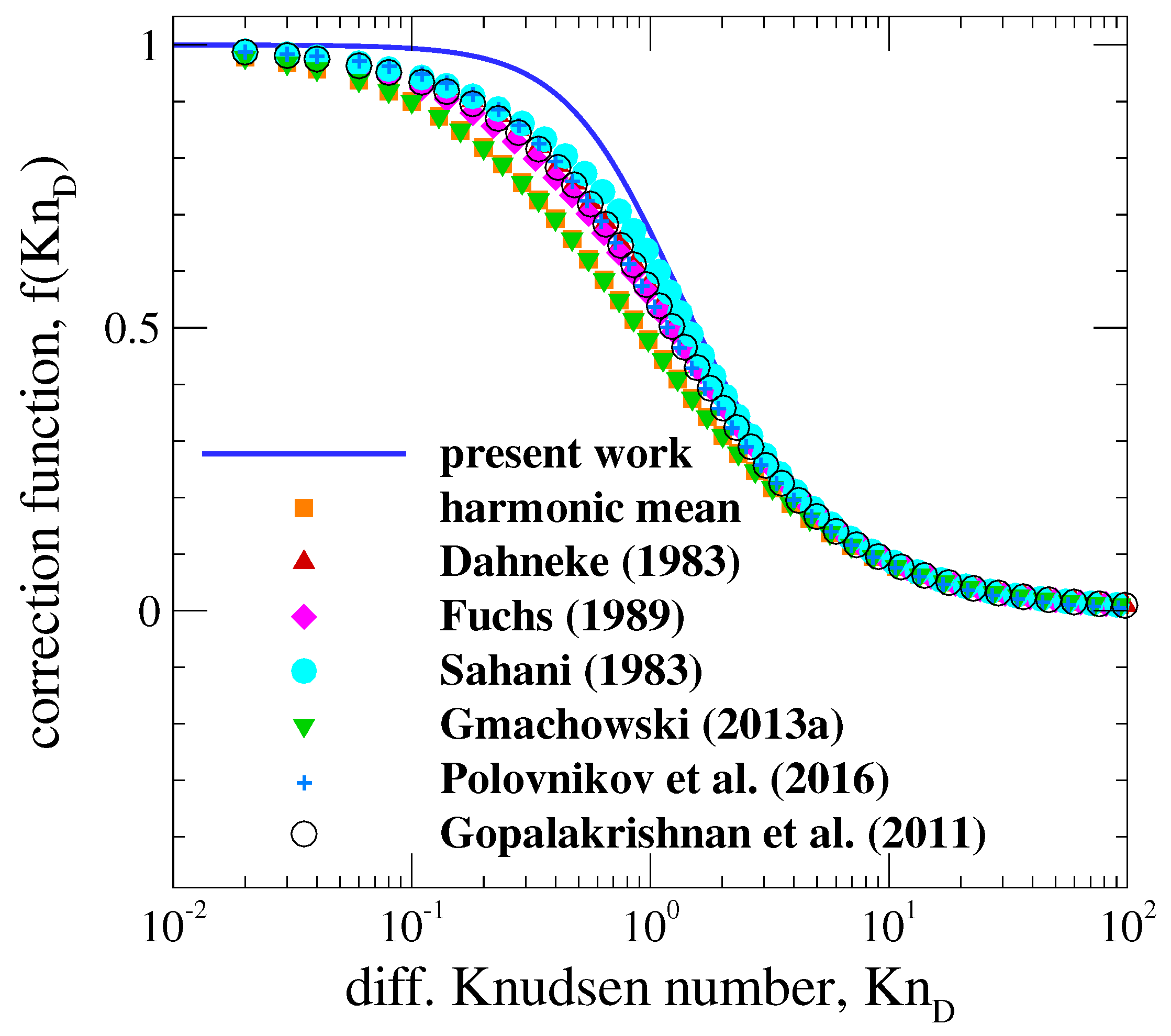
Figure 4.
(a) Coagulation kernels k as a function of the diffusive Knudsen number Kn. (b) Relative coagulation kernel compared with proposed by [12]. The proposed method, given by Equation (20) is compared with the literature. Fuchs (1989) [8], Dahneke (1983) [9], Gopalakrishnan et al. (2011) [12], Polovnikov et al. (2016) [13], Gmachowski (2013a) [14].
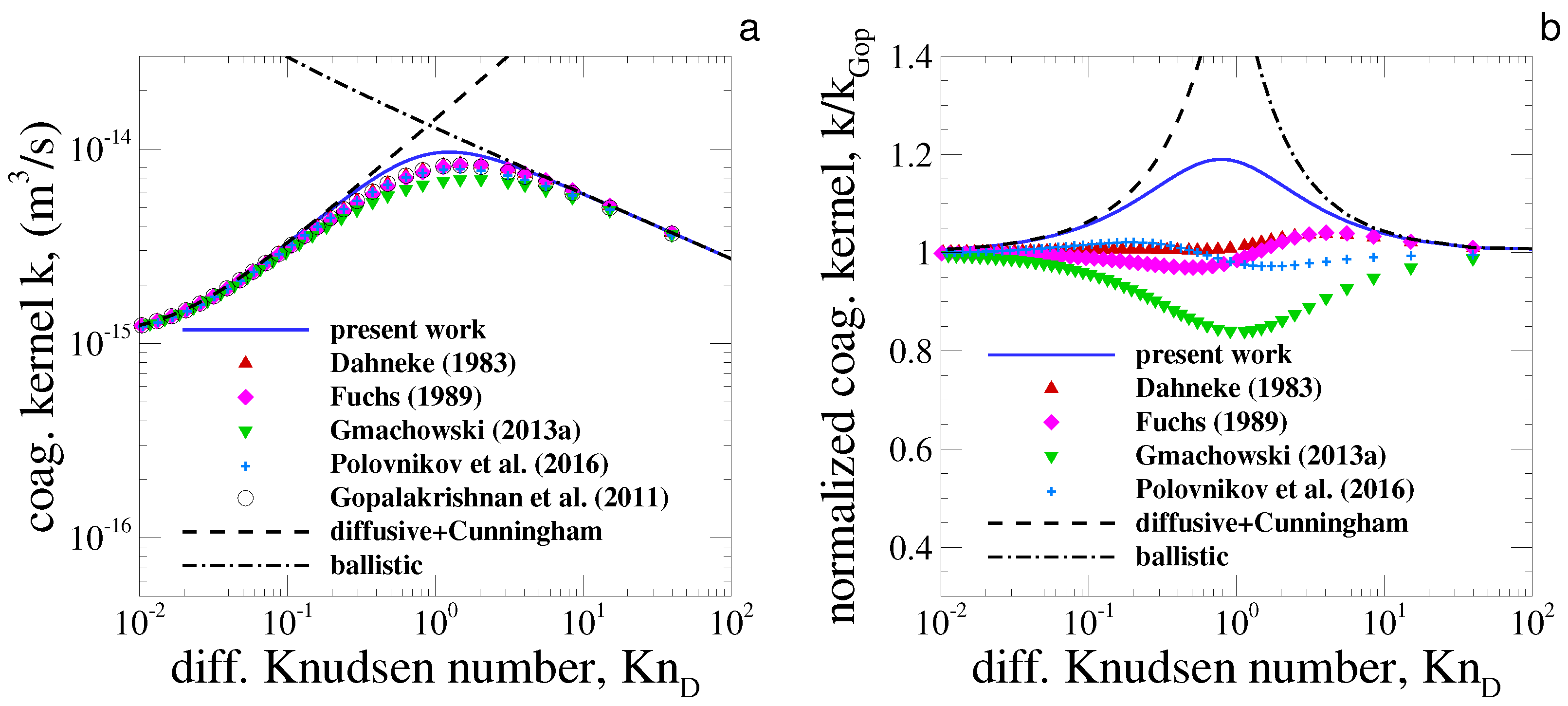
Figure 5.
The figures (a–c) represent the geometric mean (left-hand side vertical axis) and geometric standard deviation (right-hand side vertical axis) as a function of time (bottom horizontal axis) and as a function of the diffusive Knudsen number Kn (top horizontal axis). The proposed method (blue dash line) is compared with [12] (black continuous line) and the harmonic mean method, equivalent to [14] (green dash-dotted line).
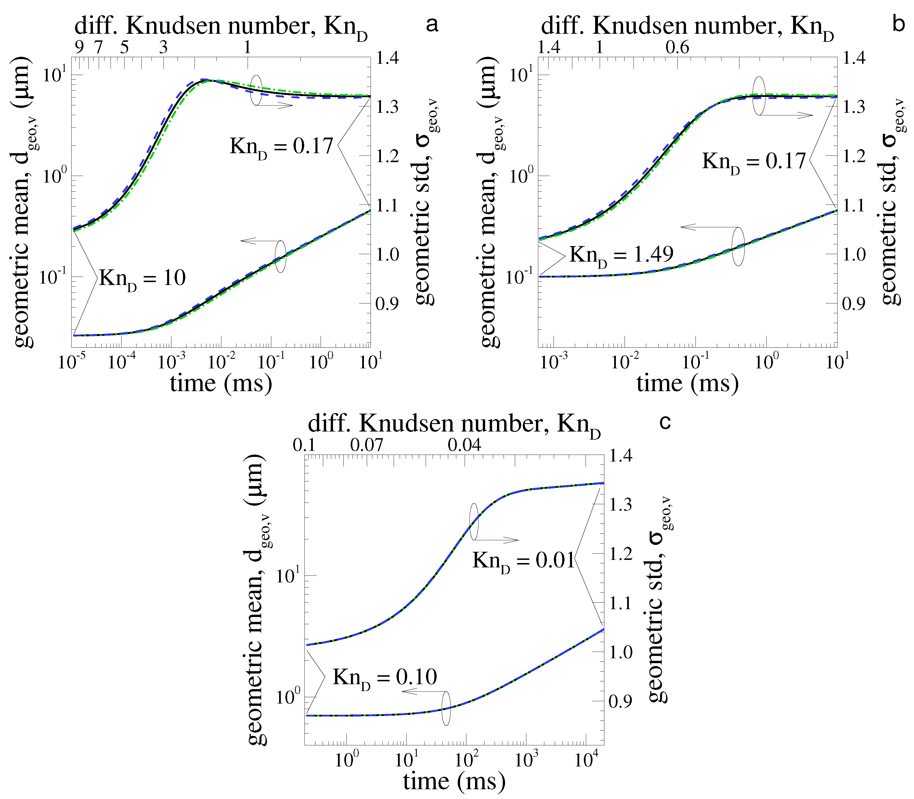
Figure 6.
The figures (a–c) represent the particle number concentration as a function of time. The proposed method (blue dash line) is compared with [12] (black continuous line) and the harmonic mean method, equivalent to [14] (green dash-dotted line).

Figure 7.
The kinetic exponent (z) of coagulating monodisperse (a) and polydisperse (b) spherical particles as a function of the diffusive Knudsen number. The volume-equivalent diameter geometric standard deviation for initially monodisperse (c) and polydisperse (d) particles is also shown. Gray filled symbols represent the z for all simulation in time. The particle diameter is indicated for each curve. The asymptotic red-dashed curve obtained by the reference method [12] is compared to the cyan continuous line obtained by using the proposed approach.

Table 1.
Different approximations of the correction function to calculate the coagulation kernels in the transition regime. The diffusive Knudsen number is given by Equation (7).
Table 1.
Different approximations of the correction function to calculate the coagulation kernels in the transition regime. The diffusive Knudsen number is given by Equation (7).
| Reference | Correction Function |
|---|---|
| Dahneke [9] | |
| Sahni [10] | |
| Fuchs [8] | |
| Gopalakrishnan et al., [12] | |
| Polovnikov et al., [13] | |
| Gmachowski [14] | |
| This work |
Publisher’s Note: MDPI stays neutral with regard to jurisdictional claims in published maps and institutional affiliations. |
© 2022 by the author. Licensee MDPI, Basel, Switzerland. This article is an open access article distributed under the terms and conditions of the Creative Commons Attribution (CC BY) license (https://creativecommons.org/licenses/by/4.0/).
Share and Cite
MDPI and ACS Style
Morán, J. On the Link between the Langevin Equation and the Coagulation Kernels of Suspended Nanoparticles. Fractal Fract. 2022, 6, 529. https://doi.org/10.3390/fractalfract6090529
AMA Style
Morán J. On the Link between the Langevin Equation and the Coagulation Kernels of Suspended Nanoparticles. Fractal and Fractional. 2022; 6(9):529. https://doi.org/10.3390/fractalfract6090529
Chicago/Turabian StyleMorán, José. 2022. "On the Link between the Langevin Equation and the Coagulation Kernels of Suspended Nanoparticles" Fractal and Fractional 6, no. 9: 529. https://doi.org/10.3390/fractalfract6090529