Artificial Neural Network for Daily Low Stream Flow Rate Prediction of Perigiali Stream, Kavala City, NE Greece †


1
Department of Civil Engineering, Democritus University of Thrace, Kimmeria Campus, 67100 Xanthi, Greece
2
Department of Mechanical Engineering, Eastern Macedonia & Thrace Institute of Technology, 65404 Kavala, Greece
*
Author to whom correspondence should be addressed.
†
Presented at the 3rd EWaS International Conference on “Insights on the Water-Energy-Food Nexus”, Lefkada Island, Greece, 27–30 June 2018.
Proceedings 2018, 2(11), 578; https://doi.org/10.3390/proceedings2110578
Published: 20 August 2018
(This article belongs to the Proceedings of EWaS3 2018)
Abstract
:Only a few scientific research studies with reference to extremely low stream flow conditions, have been conducted in Greece, so far. Forecasting future low stream flow rate values is a crucial and desicive task when conducting drought and watershed management plans, designing water reservoirs and general hydraulic works capacity, calculating hydrological and drought low flow indices, separating groundwater base flow and storm flow of storm hydrographs etc. Artificial Neural Network modeling simulation method generates artificial time series of simulated values of a random (hydrological in this specific case) variable. The present study produces artificial low stream flow time series of both a part of the past year (2016) as well as the present year (2017) considering the stream flow data observed during two different respecting interval period of the years 2016 and 2017. We compiled an Artificial Neural Network to simulate low stream flow rate data, acquired at a certain location of the partly regulated semi-urban stream which runs through the eastern exit of Kavala city, NE Greece, using a 3-inches U.S.G.S. modified portable Parshall flume, a 3-inches conventional portable Parshall flume, a 3-inches portable Montana (short Parshall) flume and a 90° V-notched triangular shaped sharp crested portable weir plate. The observed data were plotted against the predicted one and the results were demonstrated through interactive tables providing us the ability to effectively evaluate the ANN model simulation procedure performance. Finally, we plot the recorded against the simulated low stream flow rate data, compiling a log-log scale chart which provides a better visualization of the discrepancy ratio statistical performance metrics and calculate the derived model statistics featuring the comparison between the recorded and the forecasted low stream flow rate data.
1. Introduction
Low flow regimes in rivers and streams are of paramount importance to the ecological conditions of any land surface hydrological feature. Any shift in the flows pattern throughout any hydrological year, stemming, for instance, from either individual activities e.g., groundwater abstraction, precipitation shortage, riparian areas encroachment, stream channelizing due to urbanization etc., or a combination of them, may contribute to stream ecology changes that cannot be undone [1]. Low flow analysis and forecasting is also fundamental when building works along watercourses (e.g., dams, reservoirs, water deviation channels for irrigation purposes etc.) and for watercourse rehabilitation plans regarding which a knowledge of hydrological fluctuation is of fundamental importance in designing sustainable rehabilitation works.
Another type of low flow analysis, specifically probability distribution analysis, was performed in the past analyzing the observed data collected at the same gauging station between 14th of May 2016 and 31th of July 2016 revealing that Pearson type 6 (3P) demonstrated the highest final goodness of fit obtained score based, simultaneously, on all available (Anderson-Darling, Chi-Squared and Kolmogorov-Smirnov) goodness of fit criteria [2]. Furthermore, as far as the same gauging station, similar type of analysis was elaborated considering, this time, the observed data collected at the same gauging station both between 14th of May 2016 and 29th of August 2016 revealing that Wakeby type (5P) demonstrated the highest final goodness of fit obtained score based on the Kolmogorov-Smirnov goodness of fit criterion and employed to generate an artificial low flow time series for the same time interval [3,4].
Especially within the last decade, a great number of ANN models have been designed for stream flow and sediment transport rates simulation. In a scientific research article, an ANN model was employed to design a model for streamflow forecasting respecting San Juan River basin, Argentina, using meteorological data from Pachon meteorological station built at 1900 m of altitude and proved distinctively effective of fitting remarkably well the observed stream flow data [5]. In a scientific research article, an ANN model was developed and proved effective of simulating well the daily both high and low flows, in Mesochora catchment, (drained by the Acheloos River), central mountain region of Greece [6]. In another scientific research article, the performance of three different ANN Schemes (a–c) was tested in order to calculate bed load transport rate in gravel-bed rivers running within the Snake River Basin, USA [7]. In another scientific research article, an ANN model was developed and proved capable of stream flow modeling of Savitri catchment, India [8]. In another scientific research article, an ANN model was designed and performed adequately of stream flow modeling of Nestos River, NE Greece [9].
In the present scientific research study, ANNs have been employed to design a forecasting model for the daily low flows of Perigiali Stream (at the exit of the homonymous watershed), Kavala city, Eastern Macedonia & Thrace Prefecture, NE Greece. Their selection is founded on the fact that they perform remarkably well (together within other sectors of scientific interests) in the field of hydrology, although, in some occasions, there is not available adequate information respecting all the variables contributing to the watershed system driving forces.
2. Study Area
The stream flow rate gauging station established in Kavala city coastal area, is located at the north of the Aegean Sea, across the Thassos Island, and surrounded by the Lekani mountain series branches to the North and East and the Paggaion Mountain ramifications to the West, (established in the proximity of the city urban web center and at the eastern exit of the city as well), located at the specific co-ordinates 40°56′727″ N and 24°25′929″ E, Perigiali city area, and operated during specified time intervals, bridging a time interval period from 14 May 2016 to 7 October 2017, as illustrated in Figure 1. It should be noted that since it is located just a few decades of meters upstream the sea shore and simultaneously at the exit of the entire Perigiali area watershed, between the sea shore and the Old National Road connecting the eastern exit of the Kavala city to the Xanthi city, drained by the homonymous Perigiali area stream, the associated stream flow rate measurements provide profooundly valuable scientific information respecting the entire regime of the water resources, (incorporating headwaters and lower order streams to higher order streams and the main stream channel), of the Perigiali area watershed.
3. Materials and Methods
We considered the stream flow data observed during two different center interval period of the years 2016 and 2017, more precisely, during part of May (from the 14th of May 2016), June, July and part of August 2016 (until the 30th of August 2016), part of December 2016 (from the 24th of December 2016), part of January 2017 (until the 5th of January 2017) as well as part of May (from the 24th of May 2017), June, July, August, September and part of October 2017, until the 7th of October 2017, without filling the consecutive data gaps for the rest, ungauged gaps, of the years 2016 and 2017, (see supplementary materials).
The distinctively shallow waters, exacerbated by the extremely low water stream flow velocity occurring at the gauging station, make impossible to perform the area-velocity method in order to calculate the stream flow rate (discharge), using a current meter mounted on a wading rod, due to the fact that there isn’t adequate depth to submerge the current meter; Moreover, the pronounced low water stream flow velocity is not sufficient enough to trigger the operation of a current meter. Under those noticeable circumstances the only other remaining options, are the use of either a small-sized portable weir (all those its implementation brings difficulties due to the fact that weirs, in general, demand a relatively great head loss which is not available at areas in proximity to watersheds’ outlets, where, in most cases, the natural slope of the channel bed is extremely low if not zero) plate or/and a small-sized flume or/and a set of small-sized weir and flumes which, eventually, was our final selected option, more specifically, a “3-inch U.S.G.S. Modified Portable Parshall Flume”, “3-inch U.S.G.S. Conventional Portable Parshall Flume” and a “90° V-Notched Triangular-Shaped Sharp-Crested (Sharp-Edged) U.S.G.S. Portable Weir Plate” [10,11,12,13,14,15,16,17,18,19,20], made of sea plywood, covered with a sprayed thin smooth polyester coating, (identical to that usually the industry covers the outside surface of high-speed sea boats, in order to reduce the friction developing between the outside area of those sea boats and the sea water, thus securing that the friction developed between the bottom as well as the walls of the stream flow rate gauging apparatus is minimized/restricted to a minimum.
Meteorological data has been collected from Dexameni-Kavala city—Eastern Macedonia & Thrace Prefecture—Greece private meteorological station (located at 40°56′25″ N–E 24°24′01″ E, Altitude: 90 m).
Low stream flow rate values were forecasted employing MLFP that is an appropriate type of ANNs both for meteorological as well as for river stream flow rate predictions.
4. Results and Discussion
Employing MATLAB software, various different designs of MLFP were elaborated with different number of neurons within both the input as well as the hidden layers. The superb model for daily forecasting (in the present study, M13.10.1) is described within the first following subsection whilst the referenced statistical criteria are displayed within the second following one. The three important identification characteristics of the model are as following: the number of neurons in input (i), hidden (j) and output (k) layers respectively.
4.1. Structure of Artificial Neural Network (M13.10.1)
A custom neural network (abbreviated as M13.10.1) was employed in order to simulate all the 246 site-measured values of the observed stream flow rate, (as depicted within Table A1), with the following architecture: Network Type: Feed-forward back propagation, Training Function: TRAINGDX, Adaption Learning Function: LEARNGDM, Performance Function: MSE, Number of Layers: 2, Number of Neurons: 10, Transfer Function: LOGSIG. It should also be stressed that epochs was selected equal to 1000. The input data for 246 site measurements were arranged as a time series with length of 246 data.
The selected custom neural network’s architecture used for this simulation is depicted within Figure 2.
The input layer for this network consists of thirteen neurons representing total daily rainfall R, cumulative total daily rainfall RC, mean daily wind velocity UWave, maximum daily wind velocity UWmax, mean daily air temperature Tave, minimum daily air temperature Tmin, maximum daily air temperature Tmax, mean daily air humidity Have, minimum daily air humidity Hmin, maximum daily humidity Hmax, mean daily air pressure Pave, minimum daily air pressure Pmin and maximum daily pressure Pmax. For this network 10 neurons were selected for the hidden layer.
The validation performance of the ANN (M13.10.1) is illustrated within Figure 3.
The training regression performance of the ANN (M681) is illustrated within Figure 4.
4.2. Model Statistical Efficiency Criteria and Performance Metrics
The respective statistical criteria values concerning Perigiali Stream regarding the selected artificial neural network (M13.10.1) are depicted within Table 1 [21]. It is noted that the relative error value depicted within Table 1 represents the average value of the relative errors calculated for each pair of calculated and site measured low stream flow rate values.
The plot depicted within Figure 5 represents the discrepancy ratio concerning Perigiali Stream with reference to the selected artificial neural network, depicting graphically, more specifically, as far as the present study is concerned, the percentage of the computed low stream flow rate values lying between the double and the half of the corresponding recorded values. At this point, it should be noted that both coordinate axes are in logarithmic scale; therefore, the equations y = x, y = 0.5x and y = 2.0x are represented graphically by parallel straight lines [22].
In general, the obtained values of the statistical criteria RMSE, RE, EC for Perigiali Stream can be considered fairly satisfactory. Additionally, the degree of linear dependence between computed and observed low daily stream flow rate is very high.
The dates of all measurements as well as both the site measured as well as the calculated stream flow rates of Perigiali Stream are presented in Table A1.
5. Discussion-Conclusions-Further Research
Lots of models based on ANN procedure concept have been employed and proposed by researchers so far in order to model daily stream flow and sediment transport rate worldwide. In the present study, a custom neural network (abbreviated as M13.10.1) was employed in order to simulate all the 246 site-measured values of the observed low stream flow rate, (as depicted within Table A1), with the certain architecture, using as inputs several meteorological parameters, (exogenous variables of the runoff generating processes), prevailing around the study area, and turned out, among others, to be the most appropriate to simulate the recorded daily low stream flow rate data. The resulted statistical efficiency criteria proved a strong relationship between those meteorological parameters involved and the daily stream flow rate of Perigiali Stream, Kavala city, Greece, suggesting that that ANN modeling concept is able to efficiently simulate observed daily low stream flow rate data which is essential for water resources management at a watershed level in terms of drought forecasting and management, water reservoir and water deviation works design, agricultural schemes planning at a regional level, filling gaps within low stream flow rate time series, low-flow indices calculation for environmental purposes, model implementation in ungaged catchments in order to generate artificial low stream flow rate data etc. Furthermore, the fact that the observed data represents short time intervals instead of an adequately long continuous time series can be definitely considered as a limitation underlining the need of more collected low stream flow rate recorded data in order to prove that our model can be regarded as an undoubtedly reliable one. In future, provided that proper and adequate apparatus is available, we intend to monitor water quality parameters in order to perform statistical analysis and assessment [23,24] and apply stochastic models [25] to predict future respecting values which are essential towards the establishment of a holistic Perigiali watershed management scheme.
Supplementary Materials
The following are available online at https://www.youtube.com/watch?v=Wu8KBj3qqXg, Video S1: Watershed Stream Flow Measurement-Stream Perigiali-2016.06.18-Kavala City-Greece, https://www.youtube.com/watch?v=-HbPZLNGplY&feature=youtu.be, Video S2: Watershed Stream Flow Measurement-Stream Perigiali-2017.07.27(a)-Kavala City-Greece (08:16:49 a.m.).
Conflicts of Interest
The authors declare no conflict of interest.
Appendix A
The dates of all measurements as well as both the site measured as well as the calculated stream flow rates of Perigiali Stream are presented in Table A1.

Table A1.
Stream flow rate measurements of Perigiali Stream.
| No. | Date | Stream Flow Rate (m3/s) Site-Measured | Stream Flow Rate (m3/s) Calculated (M13.10.1) |
|---|---|---|---|
| 1 | 14-5-2016 | 0.4370 | 0.3151 |
| 2 | 15-5-2016 | 0.5080 | 0.5156 |
| 3 | 16-5-2016 | 0.4030 | 0.5368 |
| 4 | 17-5-2016 | 0.4030 | 0.3824 |
| 5 | 18-5-2016 | 0.4720 | 0.4206 |
| 6 | 19-5-2016 | 0.5830 | 0.3695 |
| 7 | 20-5-2016 | 0.5080 | 0.5401 |
| 8 | 21-5-2016 | 2.7460 | 2.7714 |
| 9 | 22-5-2016 | 1.0110 | 1.0422 |
| 10 | 23-5-2016 | 0.8300 | 0.7277 |
| 11 | 24-5-2016 | 0.8740 | 0.8777 |
| 12 | 25-5-2016 | 0.6620 | 0.6884 |
| 13 | 26-5-2016 | 0.6620 | 0.3522 |
| 14 | 27-5-2016 | 0.3700 | 0.3328 |
| 15 | 28-5-2016 | 0.2488 | 0.1621 |
| 16 | 29-5-2016 | 0.3701 | 0.2290 |
| 17 | 30-5-2016 | 0.2775 | 0.2464 |
| 18 | 31-5-2016 | 0.3381 | 0.2399 |
| 19 | 1-6-2016 | 0.2488 | 0.1881 |
| 20 | 2-6-2016 | 0.1700 | 0.2775 |
| 21 | 3-6-2016 | 0.3701 | 0.4214 |
| 22 | 4-6-2016 | 0.5451 | 0.3349 |
| 23 | 5-6-2016 | 0.3381 | 0.2148 |
| 24 | 6-6-2016 | 0.5450 | 0.4573 |
| 25 | 7-6-2016 | 0.3072 | 0.3277 |
| 26 | 8-6-2016 | 0.1950 | 0.3244 |
| 27 | 9-6-2016 | 0.1238 | 0.5328 |
| 28 | 10-6-2016 | 0.1238 | 0.2220 |
| 29 | 11-6-2016 | 0.1950 | 0.1596 |
| 30 | 12-6-2016 | 0.1238 | 0.2532 |
| 31 | 13-6-2016 | 1.4650 | 1.4400 |
| 32 | 14-6-2016 | 0.6220 | 0.5874 |
| 33 | 15-6-2016 | 0.4371 | 0.6716 |
| 34 | 16-6-2016 | 0.3072 | 0.3144 |
| 35 | 17-6-2016 | 0.2213 | 0.2456 |
| 36 | 18-6-2016 | 0.3072 | 0.1447 |
| 37 | 19-6-2016 | 0.2775 | 0.0960 |
| 38 | 20-6-2016 | 0.1950 | 0.1450 |
| 39 | 21-6-2016 | 0.2775 | 0.1379 |
| 40 | 22-6-2016 | 0.0832 | 0.1844 |
| 41 | 23-6-2016 | 0.1028 | 0.0345 |
| 42 | 24-6-2016 | 0.0115 | 0.0324 |
| 43 | 25-6-2016 | 0.0344 | 0.1006 |
| 44 | 26-6-2016 | 0.1462 | 0.0823 |
| 45 | 27-6-2016 | 0.1462 | 0.2139 |
| 46 | 28-6-2016 | 0.2775 | 0.3824 |
| 47 | 29-6-2016 | 0.1700 | 0.2488 |
| 48 | 30-6-2016 | 0.0652 | 0.1717 |
| 49 | 1-7-2016 | 0.1700 | 0.1751 |
| 50 | 2-7-2016 | 0.1700 | 0.1731 |
| 51 | 3-7-2016 | 0.3701 | 0.2599 |
| 52 | 4-7-2016 | 0.2775 | 0.1681 |
| 53 | 5-7-2016 | 0.2775 | 0.1840 |
| 54 | 6-7-2016 | 0.0652 | 0.1986 |
| 55 | 7-7-2016 | 0.2213 | 0.2425 |
| 56 | 8-7-2016 | 0.0218 | 0.2421 |
| 57 | 9-7-2016 | 0.0832 | 0.2085 |
| 58 | 10-7-2016 | 0.1028 | 0.1696 |
| 59 | 11-7-2016 | 0.1028 | 0.0924 |
| 60 | 12-7-2016 | 0.1028 | 0.1883 |
| 61 | 13-7-2016 | 0.0489 | 0.1802 |
| 62 | 14-7-2016 | 0.1238 | 0.2023 |
| 63 | 15-7-2016 | 0.0652 | 0.1956 |
| 64 | 16-7-2016 | 0.2213 | 0.3563 |
| 65 | 17-7-2016 | 0.1462 | 0.1511 |
| 66 | 18-7-2016 | 0.0344 | 0.2032 |
| 67 | 19-7-2016 | 0.1950 | 0.2087 |
| 68 | 20-7-2016 | 0.1028 | 0.1845 |
| 69 | 21-7-2016 | 0.0344 | 0.1792 |
| 70 | 22-7-2016 | 0.3381 | 0.1551 |
| 71 | 23-7-2016 | 0.2213 | 0.1385 |
| 72 | 24-7-2016 | 0.1950 | 0.1859 |
| 73 | 25-7-2016 | 0.1238 | 0.1675 |
| 74 | 26-7-2016 | 0.0340 | 0.2132 |
| 75 | 27-7-2016 | 0.1028 | 0.1404 |
| 76 | 28-7-2016 | 0.0489 | 0.2120 |
| 77 | 29-7-2016 | 0.0832 | 0.1716 |
| 78 | 30-7-2016 | 0.1238 | 0.1539 |
| 79 | 31-7-2016 | 0.3701 | 0.2470 |
| 80 | 1-8-2016 | 0.0652 | 0.1286 |
| 81 | 2-8-2016 | 0.1950 | 0.1875 |
| 82 | 3-8-2016 | 0.1028 | 0.2106 |
| 83 | 4-8-2016 | 0.1462 | 0.1703 |
| 84 | 5-8-2016 | 0.2488 | 0.1431 |
| 85 | 6-8-2016 | 0.3381 | 0.1404 |
| 86 | 7-8-2016 | 0.1238 | 0.1855 |
| 87 | 8-8-2016 | 0.1950 | 0.1470 |
| 88 | 9-8-2016 | 0.3701 | 0.3080 |
| 89 | 10-8-2016 | 0.1950 | 0.0914 |
| 90 | 11-8-2016 | 0.3381 | 0.1474 |
| 91 | 12-8-2016 | 0.2488 | 0.1523 |
| 92 | 13-8-2016 | 0.1950 | 0.1698 |
| 93 | 14-8-2016 | 0.2488 | 0.1911 |
| 94 | 15-8-2016 | 0.2219 | 0.2268 |
| 95 | 16-8-2016 | 0.2775 | 0.2724 |
| 96 | 17-8-2016 | 0.4371 | 0.3402 |
| 97 | 18-8-2016 | 0.3701 | 0.3989 |
| 98 | 19-8-2016 | 0.4031 | 0.3530 |
| 99 | 20-8-2016 | 0.3072 | 0.3288 |
| 100 | 21-8-2016 | 0.1950 | 0.1659 |
| 101 | 22-8-2016 | 0.2213 | 0.1439 |
| 102 | 23-8-2016 | 0.4371 | 0.1598 |
| 103 | 24-8-2016 | 0.2775 | 0.1746 |
| 104 | 25-8-2016 | 0.2213 | 0.1580 |
| 105 | 26-8-2016 | 0.2775 | 0.3003 |
| 106 | 27-8-2016 | 0.2775 | 0.4087 |
| 107 | 28-8-2016 | 0.3072 | 0.2810 |
| 108 | 29-8-2016 | 0.4371 | 0.1957 |
| 109 | 30-8-2016 | 0.6616 | 0.1487 |
| 110 | 24-5-2017 | 0.1210 | 0.0630 |
| 111 | 25-5-2017 | 0.0820 | 0.2088 |
| 112 | 26-5-2017 | 5.9150 | 5.8006 |
| 113 | 27-5-2017 | 0.2130 | 0.3294 |
| 114 | 28-5-2017 | 0.0820 | 0.0721 |
| 115 | 29-5-2017 | 0.0650 | 0.1313 |
| 116 | 30-5-2017 | 0.1010 | 0.0732 |
| 117 | 31-5-2017 | 0.0490 | 0.0942 |
| 118 | 1-6-2017 | 0.0340 | 0.0577 |
| 119 | 2-6-2017 | 0.0650 | 0.0701 |
| 120 | 3-6-2017 | 0.0650 | 0.0926 |
| 121 | 4-6-2017 | 0.0820 | 0.1520 |
| 122 | 5-6-2017 | 0.0650 | 0.1203 |
| 123 | 6-6-2017 | 0.0820 | 0.1310 |
| 124 | 7-6-2017 | 0.0650 | 0.0775 |
| 125 | 8-6-2017 | 0.0820 | 0.0967 |
| 126 | 9-6-2017 | 0.1010 | 0.2323 |
| 127 | 10-6-2017 | 0.0820 | 0.0822 |
| 128 | 11-6-2017 | 5.8560 | 5.7520 |
| 129 | 12-6-2017 | 1.4010 | 0.1787 |
| 130 | 13-6-2017 | 0.0650 | 0.1244 |
| 131 | 14-6-2017 | 0.1010 | 0.0562 |
| 132 | 15-6-2017 | 0.0820 | 0.0934 |
| 133 | 16-6-2017 | 0.0820 | 0.1727 |
| 134 | 17-6-2017 | 0.1010 | 0.0953 |
| 135 | 18-6-2017 | 0.0820 | 0.2393 |
| 136 | 19-6-2017 | 0.0650 | 0.1153 |
| 137 | 20-6-2017 | 0.0650 | 0.2136 |
| 138 | 21-6-2017 | 0.0650 | 0.0858 |
| 139 | 22-6-2017 | 0.0650 | 0.1791 |
| 140 | 23-6-2017 | 0.0650 | 0.0815 |
| 141 | 24-6-2017 | 0.0490 | 0.0913 |
| 142 | 25-6-2017 | 0.0650 | 0.0944 |
| 143 | 26-6-2017 | 0.0490 | 0.1180 |
| 144 | 27-6-2017 | 0.0490 | 0.1054 |
| 145 | 28-6-2017 | 0.0490 | 0.0907 |
| 146 | 29-6-2017 | 0.0490 | 0.0868 |
| 147 | 30-6-2017 | 0.0490 | 0.0799 |
| 148 | 1-7-2017 | 0.0490 | 0.0761 |
| 149 | 2-7-2017 | 0.0490 | 0.0405 |
| 150 | 3-7-2017 | 0.0645 | 0.0220 |
| 151 | 4-7-2017 | 0.0486 | 0.0528 |
| 152 | 5-7-2017 | 0.0486 | 0.0771 |
| 153 | 6-7-2017 | 0.0486 | 0.1173 |
| 154 | 7-7-2017 | 0.0486 | 0.0557 |
| 155 | 8-7-2017 | 0.0486 | 0.0526 |
| 156 | 9-7-2017 | 0.0486 | 0.0943 |
| 157 | 10-7-2017 | 0.0344 | 0.0954 |
| 158 | 11-7-2017 | 0.0344 | 0.1002 |
| 159 | 12-7-2017 | 0.0645 | 0.1101 |
| 160 | 13-7-2017 | 0.0344 | 0.0953 |
| 161 | 14-7-2017 | 0.9872 | 0.0938 |
| 162 | 15-7-2017 | 0.1007 | 0.1689 |
| 163 | 16-7-2017 | 0.0819 | 0.0594 |
| 164 | 17-7-2017 | 0.1421 | 0.1343 |
| 165 | 18-7-2017 | 0.1208 | 0.0546 |
| 166 | 19-7-2017 | 0.1007 | 0.1309 |
| 167 | 20-7-2017 | 0.0819 | 0.1488 |
| 168 | 21-7-2017 | 0.0486 | 0.1666 |
| 169 | 22-7-2017 | 0.0645 | 0.0871 |
| 170 | 23-7-2017 | 0.0645 | 0.0853 |
| 171 | 24-7-2017 | 0.0645 | 0.0791 |
| 172 | 25-7-2017 | 0.0344 | 0.0470 |
| 173 | 26-7-2017 | 0.0486 | 0.0324 |
| 174 | 27-7-2017 | 0.0486 | 0.1451 |
| 175 | 28-7-2017 | 0.0486 | 0.0401 |
| 176 | 29-7-2017 | 0.0486 | 0.0833 |
| 177 | 30-7-2017 | 0.0486 | 0.0854 |
| 178 | 31-7-2017 | 0.0486 | 0.0917 |
| 179 | 1-8-2017 | 0.0344 | 0.1454 |
| 180 | 2-8-2017 | 0.0344 | 0.1289 |
| 181 | 3-8-2017 | 0.0344 | 0.0650 |
| 182 | 4-8-2017 | 0.0344 | 0.0745 |
| 183 | 5-8-2017 | 0.0344 | 0.0478 |
| 184 | 6-8-2017 | 0.0486 | 0.0646 |
| 185 | 7-8-2017 | 0.0344 | 0.0831 |
| 186 | 8-8-2017 | 0.0344 | 0.0593 |
| 187 | 9-8-2017 | 0.0344 | 0.0648 |
| 188 | 10-8-2017 | 0.0344 | 0.0761 |
| 189 | 11-8-2017 | 0.0344 | 0.0717 |
| 190 | 12-8-2017 | 0.0344 | 0.0536 |
| 191 | 13-8-2017 | 0.0344 | 0.0579 |
| 192 | 14-8-2017 | 0.0344 | 0.0325 |
| 193 | 15-8-2017 | 0.0344 | 0.0407 |
| 194 | 16-8-2017 | 0.0344 | 0.0666 |
| 195 | 17-8-2017 | 0.0344 | 0.0412 |
| 196 | 18-8-2017 | 0.0221 | 0.0871 |
| 197 | 19-8-2017 | 0.2060 | 0.0963 |
| 198 | 20-8-2017 | 0.1890 | 0.0784 |
| 199 | 21-8-2017 | 0.1670 | 0.0463 |
| 200 | 22-8-2017 | 0.0486 | 0.1150 |
| 201 | 23-8-2017 | 0.1210 | 0.0395 |
| 202 | 24-8-2017 | 0.0486 | 0.0695 |
| 203 | 25-8-2017 | 0.0486 | 0.0432 |
| 204 | 26-8-2017 | 0.2070 | 0.0584 |
| 205 | 27-8-2017 | 0.1690 | 0.0670 |
| 206 | 28-8-2017 | 0.0344 | 0.0642 |
| 207 | 29-8-2017 | 0.0486 | 0.0653 |
| 208 | 30-8-2017 | 0.1770 | 0.1272 |
| 209 | 31-8-2017 | 0.1710 | 0.0511 |
| 210 | 1-9-2017 | 0.0730 | 0.0719 |
| 211 | 2-9-2017 | 0.0470 | 0.0651 |
| 212 | 3-9-2017 | 0.1930 | 0.0619 |
| 213 | 4-9-2017 | 0.9439 | 0.0466 |
| 214 | 5-9-2017 | 0.0344 | 0.0558 |
| 215 | 6-9-2017 | 0.0360 | 0.0309 |
| 216 | 7-9-2017 | 0.0320 | 0.0423 |
| 217 | 8-9-2017 | 0.0430 | 0.1097 |
| 218 | 9-9-2017 | 0.1390 | 0.1766 |
| 219 | 10-9-2017 | 0.1370 | 0.1078 |
| 220 | 11-9-2017 | 0.0220 | 0.0488 |
| 221 | 12-9-2017 | 0.0344 | 0.0442 |
| 222 | 13-9-2017 | 0.1450 | 0.0686 |
| 223 | 14-9-2017 | 0.0344 | 0.1917 |
| 224 | 15-9-2017 | 0.1610 | 0.1379 |
| 225 | 16-9-2017 | 0.1490 | 0.0648 |
| 226 | 17-9-2017 | 0.0486 | 0.0852 |
| 227 | 18-9-2017 | 0.1080 | 0.0699 |
| 228 | 19-9-2017 | 0.0486 | 0.0667 |
| 229 | 20-9-2017 | 0.0344 | 0.0622 |
| 230 | 21-9-2017 | 0.0990 | 0.0127 |
| 231 | 22-9-2017 | 0.0714 | 0.0565 |
| 232 | 23-9-2017 | 0.1380 | 0.0165 |
| 233 | 24-9-2017 | 0.0996 | 0.0243 |
| 234 | 25-9-2017 | 0.0934 | 0.1726 |
| 235 | 26-9-2017 | 4.6003 | 4.6082 |
| 236 | 27-9-2017 | 0.1870 | 0.0140 |
| 237 | 28-9-2017 | 0.1510 | 0.0125 |
| 238 | 29-9-2017 | 0.1790 | 0.0118 |
| 239 | 30-9-2017 | 0.0330 | 0.0174 |
| 240 | 1-10-2017 | 0.1280 | 0.1406 |
| 241 | 2-10-2017 | 0.1420 | 0.0136 |
| 242 | 3-10-2017 | 0.0910 | 0.0124 |
| 243 | 4-10-2017 | 0.0650 | 0.0139 |
| 244 | 5-10-2017 | 0.1050 | 0.0147 |
| 245 | 6-10-2017 | 0.0590 | 0.0550 |
| 246 | 7-10-2017 | 1.1245 | 1.1225 |
References
- Gustard, A.; Demuth, S. Estimating, Predicting and Forecasting Low Flows. In Manual on Low-flow Estimation and Prediction (Operational Hydrology Report No. 50), 1st ed.; Gustard, A., Demuth, S., Eds.; World Meteorological Organization (WMO): Geneva, Switzerland, 2008; Volume 1029, pp. 16–21. [Google Scholar]
- Papalaskaris, T.; Panagiotidis, T. Artificial Low Stream Flow Time Series Generation of Perigiali Stream, Kavala city, NE Greece. In Proceedings of the 6th International Symposium on Environmental & Material Flow Management (6th E.M.F.M.), Bor, Serbia, 2–4 October 2016; Živković, Ž., Mihajlović, I., Dordević, P., Eds.; University of Belgrade, Technical Faculty in Bor: Bor, Serbia, 2016; pp. 20–38. [Google Scholar]
- Papalaskaris, T.; Panagiotidis, T. Stochastic generation of low stream flow data of Perigiali Stream, Kavala city, NE Greece. In Proceedings of the 10th World Congress of European Water Resources Association (“E.W.R.A.”) on Water Resources and Environment “Panta Rhei” (10th “E.W.R.A.” “Panta Rhei”), Athens, Greece, 5–9 July 2017; Tsakiris, G., Tsihrintzis, V., Vangelis, H., Tigkas, D., Eds.; European Water Resources Association (E.W.R.A.): Athens, Greece, 2017; pp. 953–960. [Google Scholar]
- Papalaskaris, T.; Panagiotidis, T. Stochastic generation of low stream flow data of Perigiali Stream, Kavala city, NE Greece. Eur. Water 2017, 60, 299–306. [Google Scholar] [CrossRef]
- Dolling, O.; Varas, E. Artificial neural networks for streamflow prediction. J. Hydraul. Res. 2002, 40, 547–554. [Google Scholar] [CrossRef]
- Panagoulia, D. Artificial neural networks and high and low flows in various climate regimes. Hydrol. Sci. J. 2006, 51, 563–587. [Google Scholar] [CrossRef]
- Kitsikoudis, V.; Sidiropoulos, E.; Hrissanthou, V. Machine Learning Utilization for Bed Load Transport in Gravel-Bed Rivers. Water Resour. Manag. 2014, 28, 3727–3743. [Google Scholar] [CrossRef]
- Kothari, M.; Gharde, K.D. Application of ANN and fuzzy logic algorithms for stream flow modeling of Savitri catchment. J. Earth Syst. Sci. 2015, 124, 933–943. [Google Scholar] [CrossRef]
- Papalaskaris, T.; Dimitriadou, P. Artificial Neural Network for Bed Load Transport Rate in Nestos River, Greece. Spec. Top. Rev. Porous Media Int. J. 2017, 8, 145–157. [Google Scholar] [CrossRef]
- Johnson, A. Modified Parshall Flume (U.S. Geological Survey Open-File Report), 1st ed.; United States Department of the Interior Geological Survey: Denver, CO, USA, 1963; pp. 1–8.
- Survey, G.; Rantz, S.E. In Measurement and Computation of Streamflow: Volume 1. Measurement of Stage and Discharge, 1st ed.; United States Government Printing Office: Washington, DC, USA, 1982; Volume 1, pp. 260–272.
- Modified Parshall Flume—(U.S.G.S.). Available online: https://www.usgs.gov/media/images/modified-parshall-flume (accessed on 3 March 2018).
- U.S.G.S. Portable Parshall Flume (Open-Channel-Flow Hydrological Equipment). Available online: https://www.openchannelflow.com/blog/usgs-portable-parshall-flume (accessed on 3 March 2018).
- U.S.G.S. Portable Parshall Flume, 3in (Rickly Hydrological Equipment). Available online: http://rickly.com/usgs-portable-parshall-flume-3in/ (accessed on 3 March 2018).
- Measuring Low Flow in San Pedro River. Available online: https://www.youtube.com/watch?v=gLWtfMYicrI (accessed on 3 March 2018).
- Inspecting a Parshall Flume (3-Inch USGS Modified Portable). Available online: https://www.youtube.com/watch?v=YtqflgfOb5E (accessed on 3 March 2018).
- Inspecting a Parshall Flume. Available online: https://www.youtube.com/watch?v=y6hiOLgTo6g (accessed on 3 March 2018).
- Inspecting a Parshall Flume (a+b). Available online: https://www.youtube.com/watch?v=EgV5AKAYBe4 (accessed on 3 March 2018).
- MSc. In Management of Water Resources in the Mediterranean 3. Available online: https://www.youtube.com/watch?v=picUMHITkx0 (accessed on 3 March 2018).
- Father of the Flume: Ralph Parshall. Available online: https://lib2.colostate.edu/archives/water/parshall/ (accessed on 3 March 2018).
- Krause, P.; Boyle, D.P.; Bäse, F. Comparison of different efficiency criteria for hydrological model assessment. Adv. Geosci. 2005, 5, 89–97. [Google Scholar] [CrossRef]
- Papalaskaris, T.; Dimitriadou, P.; Hrissanthou, V. Comparison between computations and measurements of bed load transport rate in Nestos River, Greece. Procedia Eng. 2016, 162, 172–180. [Google Scholar] [CrossRef]
- Sentas, A.; Psilovikos, A.; Psilovikos, T. Statistical Analysis and Assessment of Water Quality Parameters in Pagoneri, River Nestos. Eur. Water 2016, 55, 115–124. Available online: http://www.ewra.net/ew/pdf/EW_2016_55_10.pdf (accessed on 10 May 2018).
- Sentas, A.; Psilovikos, A. Monitoring Parameters Tw, DO and Environmental Evaluation of the Artificial Lake of Thesaurus for the years 2004–2007. In Proceedings of the 1st International Conference HydroMedit 2014, Volos, Greece, 13–15 November 2014; Department of Ichthyology & Aquatic Environment, University of Thessaly: Volos, Greece, 2014; pp. 19–23. [Google Scholar]
- Sentas, A.; Psilovikos, A.; Matzafleri, N. Application of stochastic models for predicting water quality in Dam-Lake Thesaurus, Greece. In Proceedings of the 12th International Conference: Protection and Restoration of the Environment XII, Skiathos, Greece, 29 June–3 July 2014; Kanakoudis, V., Theodoros, Karakasidis, E., Laspidou, C., Kungolos, A., Samaras, P., Eds.; Desalination & Water Treatment Journal: London, UK, 2016; Volume 57, 11435. pp. 458–465. [Google Scholar]
Figure 1.
Parshall flumes and V-Notched weir gauging station, Perigiali Stream area, Kavala city, Greece.
Figure 1.
Parshall flumes and V-Notched weir gauging station, Perigiali Stream area, Kavala city, Greece.

Figure 2.
ANN (M13.10.1) architecture plot of Perigiali Stream.
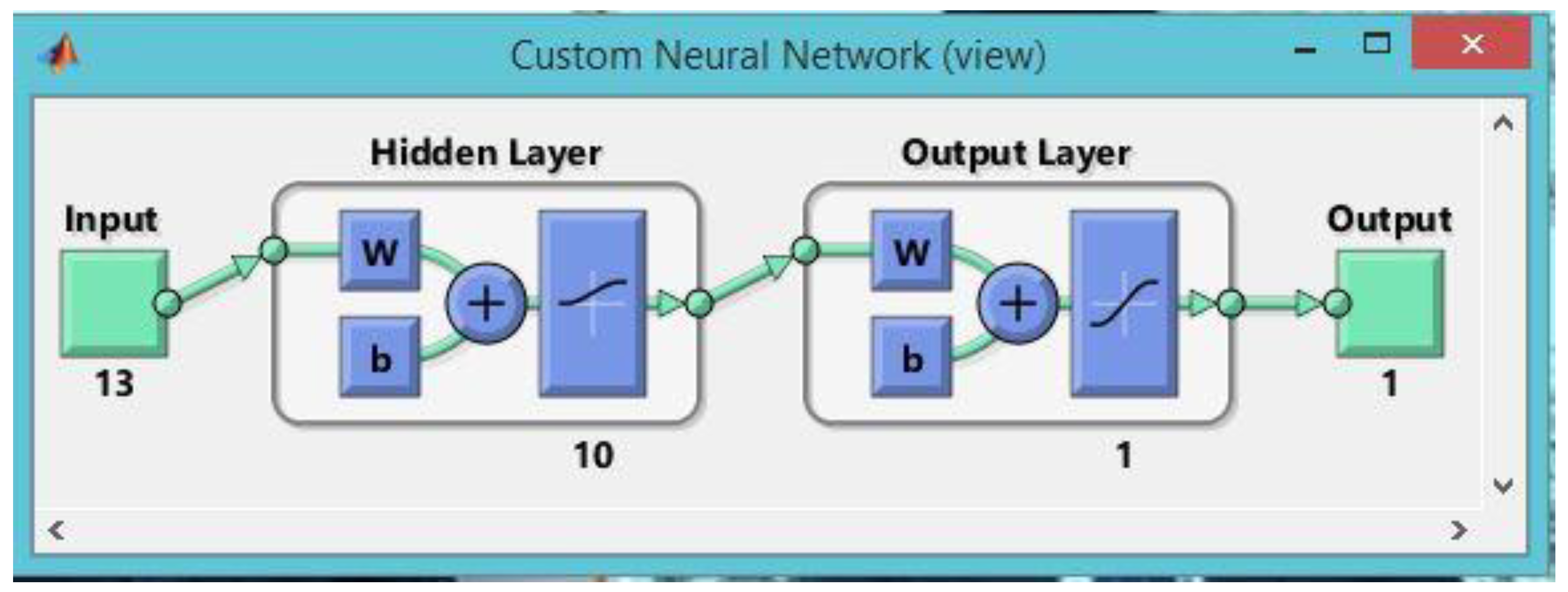
Figure 3.
ANN (M13.10.1) validation performance plot of Perigiali Stream.

Figure 4.
ANN (M13.10.1) training regression performance plots of Perigiali Stream.
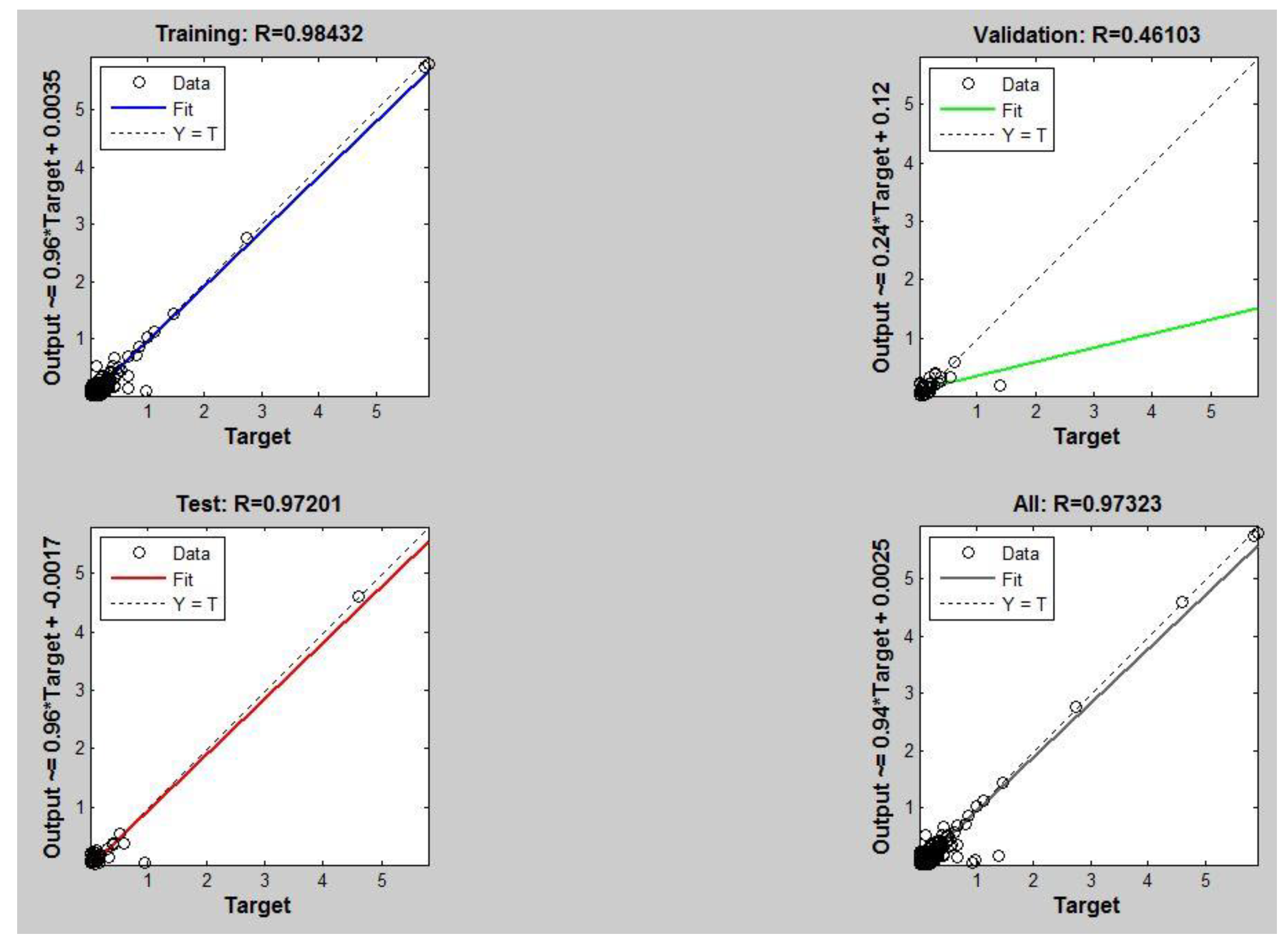
Figure 5.
Discrepancy ratio plot of Perigiali Stream (ANN M13.10.1).

Table 1.
Statistical criteria values of Perigiali Stream (ANN M13.10.1).
| Number of Paired Values | RMSE (ltrs/s) | RE (%) | EC | r | r2 | Discrepancy Ratio |
|---|---|---|---|---|---|---|
| 246 | 0.1479 | −0.4080 | 0.9468 | 0.9732 | 0.9472 | 0.6789 |
Publisher’s Note: MDPI stays neutral with regard to jurisdictional claims in published maps and institutional affiliations. |
© 2018 by the authors. Licensee MDPI, Basel, Switzerland. This article is an open access article distributed under the terms and conditions of the Creative Commons Attribution (CC BY) license (https://creativecommons.org/licenses/by/4.0/).
Share and Cite
MDPI and ACS Style
Papalaskaris, T.; Panagiotidis, T. Artificial Neural Network for Daily Low Stream Flow Rate Prediction of Perigiali Stream, Kavala City, NE Greece. Proceedings 2018, 2, 578. https://doi.org/10.3390/proceedings2110578
AMA Style
Papalaskaris T, Panagiotidis T. Artificial Neural Network for Daily Low Stream Flow Rate Prediction of Perigiali Stream, Kavala City, NE Greece. Proceedings. 2018; 2(11):578. https://doi.org/10.3390/proceedings2110578
Chicago/Turabian StylePapalaskaris, Thomas, and Theologos Panagiotidis. 2018. "Artificial Neural Network for Daily Low Stream Flow Rate Prediction of Perigiali Stream, Kavala City, NE Greece" Proceedings 2, no. 11: 578. https://doi.org/10.3390/proceedings2110578