Proceeding Paper

Ionospheric Effects of Natural Hazards in Geophysics: From Single Examples to Statistical Studies Applied to M5.5+ Earthquakes †

1
College of Instrumentation and Electrical Engineering, Jilin University, Changchun 130061, China
2
Space Observation Research Center, National Institute of Natural Hazards, Ministry of Emergency Management of China, Beijing 100085, China
3
National Space Science Center, Chinese Academy of Sciences, Beijing 100085, China
*
Author to whom correspondence should be addressed.
Presented at the 4th International Electronic Conference on Geosciences, 1–15 December 2022; Available online: https://sciforum.net/event/IECG2022.
Proceedings 2023, 87(1), 34; https://doi.org/10.3390/IECG2022-13826
Published: 7 December 2022
(This article belongs to the Proceedings of The 4th International Electronic Conference on Geosciences)

Abstract

:
Geophysical natural hazards, such as earthquakes and volcano eruptions, can have catastrophic effects on the population depending on the location and quality of construction. From the geophysical point of view, several aspects are still debated in the preparation phase of such events. In particular, several theories propose that prior to an earthquake or volcano eruption, the releases of gas, fluids or charged particles from the lithosphere (e.g., from the fault for the earthquake) could create some effects on the atmosphere and ionosphere. In this work, several single examples will be shown of possible candidates of pre-earthquake ionospheric disturbances recorded by the China National Space Administration (in partnership with the Italian Space Agency), China Seismo Electromagnetic Satellite (CSES) and European Space Agency Swarm constellation. The examples show anomalous ionospheric status in terms of magnetic disturbances or increase of electron density before earthquakes, such as Mw = 7.1 Ridgecrest (US) 2019, or during the large recent volcano eruption of Hunga Tonga-Hunga Ha’Apai on 15 January 2022. In these cases, some couplings between the lithosphere and ionosphere are proposed. Finally, verifying if such pre-event ionospheric disturbances are by “chance” or are really linked to the incoming event is a crucial point. For this purpose, we perform worldwide statistical studies, not only supporting the recurrence of such phenomena for about 15% of M5.5+ shallow earthquakes but also showing a link between the magnitude of the upcoming seismic events and the pre-earthquake anticipation time. Furthermore, we also show the influence of the location (sea or land) on the frequency of the ionospheric electromagnetic disturbance.

1. Introduction

The existence of ionospheric pre-earthquake electromagnetic disturbances is a controversial topic among researchers. Despite the scepticism of some researchers, several pieces of evidence exist of such disturbances. In particular, several single-earthquake studies provide empirical evidence for ionospheric anomalies before large earthquakes worldwide; for example, Mansouri et al. [1] showed perturbations before the M8.3 Chile 2015 earthquake. In addition, statistical studies, particularly on the DEMETER satellite that flew from 2004 to 2010, provided proof that shallow M4.8+ earthquakes were statistically preceded by electron density anomalies in the 15 days before the earthquakes [2,3]. Several Lithosphere, Atmosphere, and Ionosphere Coupling (LAIC) models support pre-earthquake ionospheric disturbances. Unfortunately, there is no unique LAIC model. In the present state of the art, it is unclear if the various models describe several different coupling mechanisms or if some of them are wrong. They are based on a chain of phenomena that starts with the air ionisation induced by radon released from the fault (e.g., Pulinets and Ouzounov [4]); the generation of positive holes (p-holes) as suggested by Freund [5]; a direct electromagnetic ULF emission from the micro-crack as suggested by Molchanov and Hayakawa [6] or even the Acoustic Gravity Waves induced by thermal heating of the Earth’s surface [7].
This short paper will present a few examples of ionospheric pre-earthquake and -volcano ionospheric disturbances and, finally, a systematical statistical investigation of China Seismo Electromagnetic Satellite (CSES) electron density and M5.5+ earthquakes which supports the existence of such pre-earthquake phenomena.
All of the earthquake analyses were performed inside a circular area that scales exponentially with the moment magnitude as defined by Dobrovoslky et al. [8].

2. Results

Here, we present some examples of anomalies before two earthquakes: Mw = 8.3 Chile 2015 and Mw = 7.1 Ridgecrest (US) 2019, and during and after the large Volcanic Explosive Index (VEI) = 6 Hunga Tonga-Hunga Ha’apai eruption of 15 January 2022.

2.1. Mw = 8.3 Illapel (Chile) 16 September 2015 Earthquake

On 16 September 2015 at 22:54:32 UT, a large earthquake of moment magnitude Mw = 8.3 hit Chile close to Illapel, with its epicentre localised at 31.573° S, 71.674° W. To date, this is the largest earthquake that has occurred during the ESA Swarm mission. De Santis et al. [9] studied the Swarm magnetic and electron density data one month before and after the earthquake, together with 11 other seismic events with a magnitude of 6.1 or greater. The most interesting result of this paper is the correlation between the number of detected magnetic or electron density anomalies and earthquake magnitude. Despite this, such a study was limited to analysing only one month before the earthquake. At the same time, several other investigations provide evidence for anomalies even before this, particularly for large earthquakes [10,11,12]. For this purpose, in Figure 1 and Figure 2, we show an example of an anomaly in the magnetic field, especially in the Y-East component that appeared about 258 days before the mainshock, very close to the future epicentre. Such anomaly has a magnetic conjugate with slightly lower intensity and shorter, supporting the hypothesis that the anomaly’s source was above the epicentre and it propagated in the conjugated point following geomagnetic field lines, losing part of the energy as predicted by the theories [13]. Looking at the following tracks, we still notice the presence of the anomaly in the Y-East component in track 11 fully inside the Dobrosvolsky area and still close to the future epicentre (slightly shifted northward according to the magnetic field direction). Contrariwise, even though we detected a clear anomaly outside the Dobrovolsky area in track 13 (green line in Figure 2), its shape is totally different. In fact, it presents a larger intensity far from the centre of the anomaly, similar to a butterfly shape, so we believe this is likely another source compared to the phenomenon depicted in Tracks 9 and 11 inside the Dobrovolsky area.

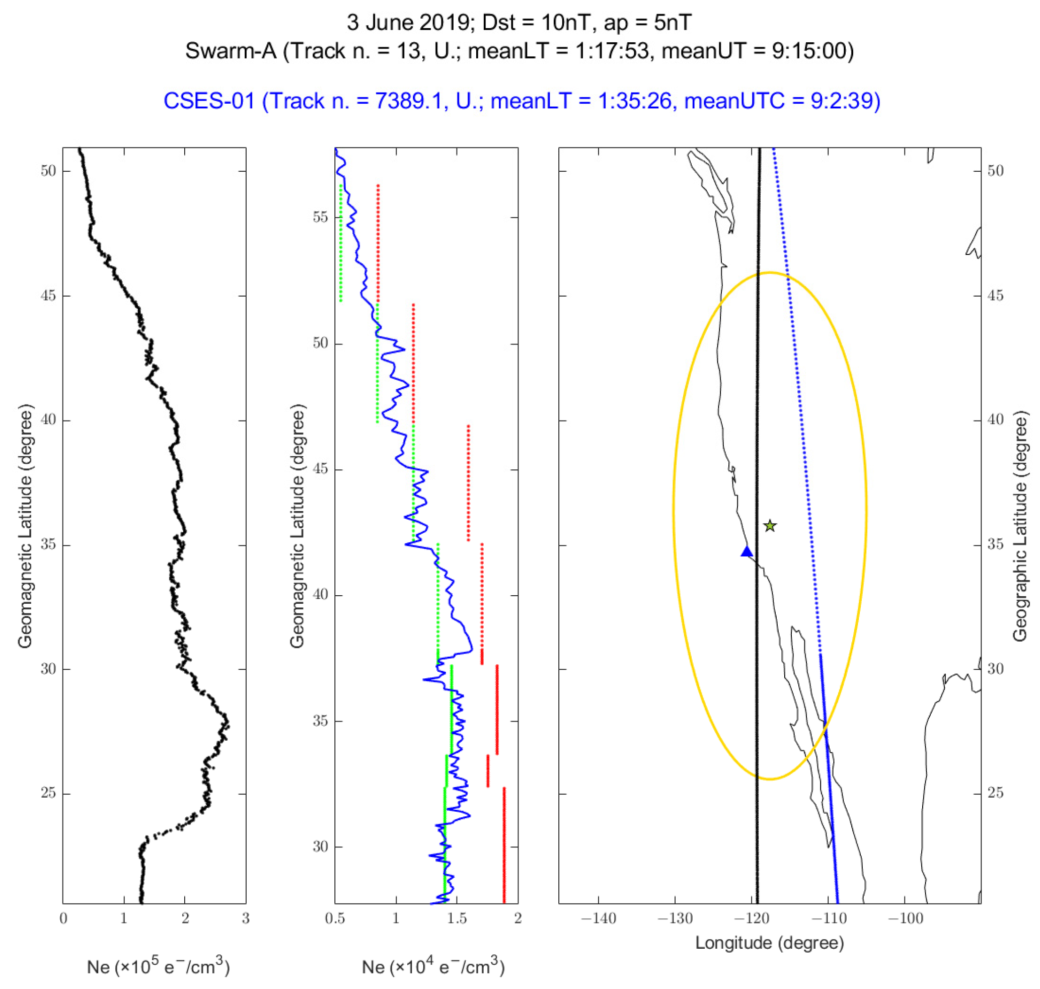
2.2. Mw = 7.1 Ridgecrest (California, US) 6 July 2019 Earthquake

On 6 July 2019 at 3:19:53 UT, an earthquake of moment magnitude 7.1 was localised close to Ridgecrest in California (US). It was a result of the strike-slip focal mechanism, and its depth was estimated at ~8.0 km. De Santis et al. [14] claimed a chain of processes compatible with a LAIC and characteristics of complex systems, such as earthquakes. Furthermore, an increase of magnetic anomalies was detected by Swarm satellites about 220 days before the earthquake by Marchetti et al. [15], and anomalies in Total Electron Content and CSES-01 Ne data about one week before the mainshock by Xie et al. [16]. In addition, De Santis et al. [14] identified an increase of electron density 33 days prior to the mainshock as unique in several months of data investigation from Point Arguello ionosonde (whose position is represented by the blue triangle in the map in Figure 3) and Swarm Alpha, here reported in Figure 3. We also checked the electron density recorded by CSES-01 on the same night at a very short time difference (just 13 min before). The CSES satellite did not record any anomalous electron density value.
This apparent discrepancy can be explained in two different ways. The first is that the increase of electron density occurred only westward of the future epicentre. The second explanation could be that such an electron density increase, theorised to come from the internal layer (the lithosphere), did not reach the higher altitude of the CSES satellite (about 510 km) compared with that of Swarm Alpha at that time (about 470 km). We tend to exclude the possibility that the ionosphere could have changed in a much shorter time.

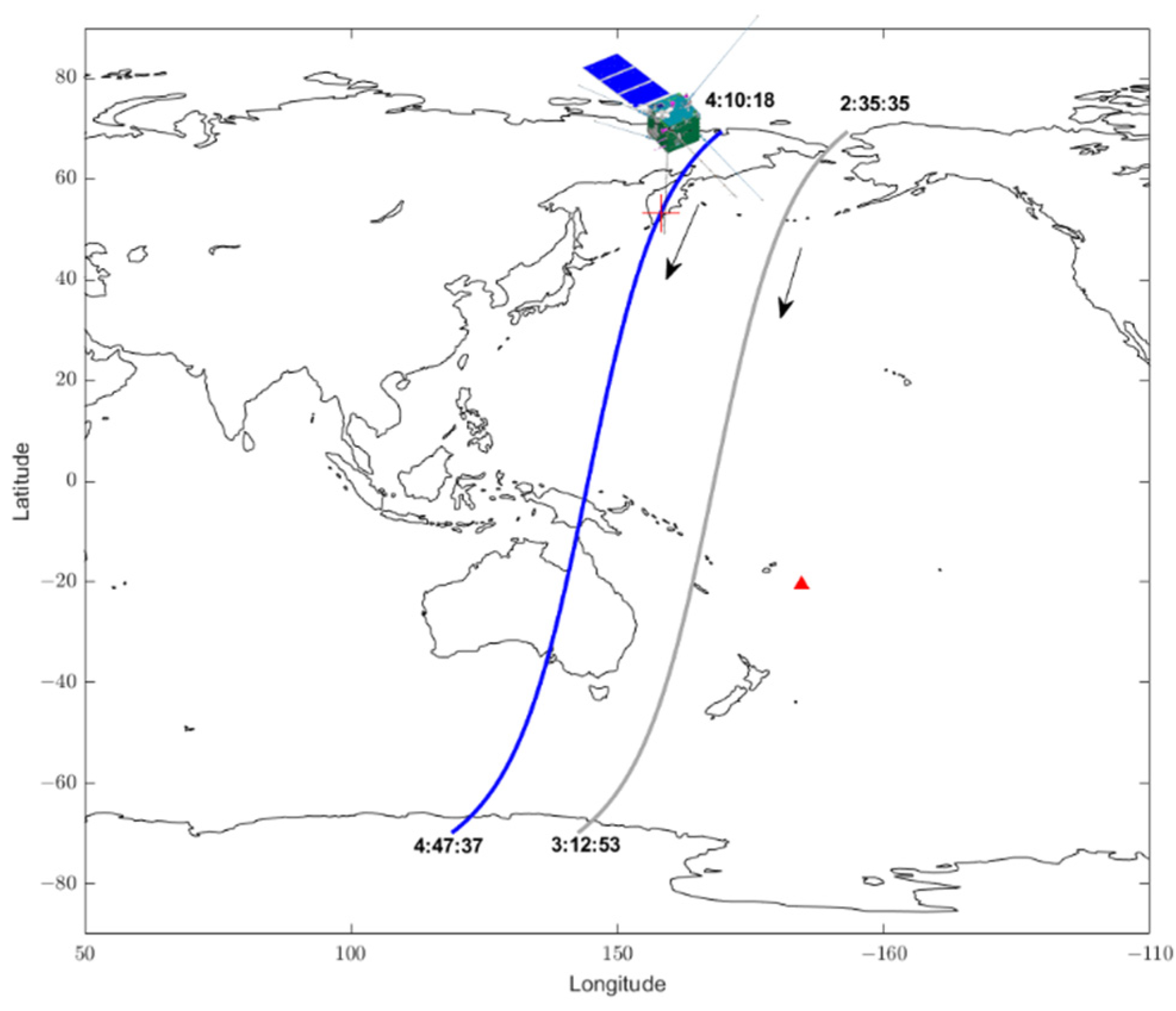
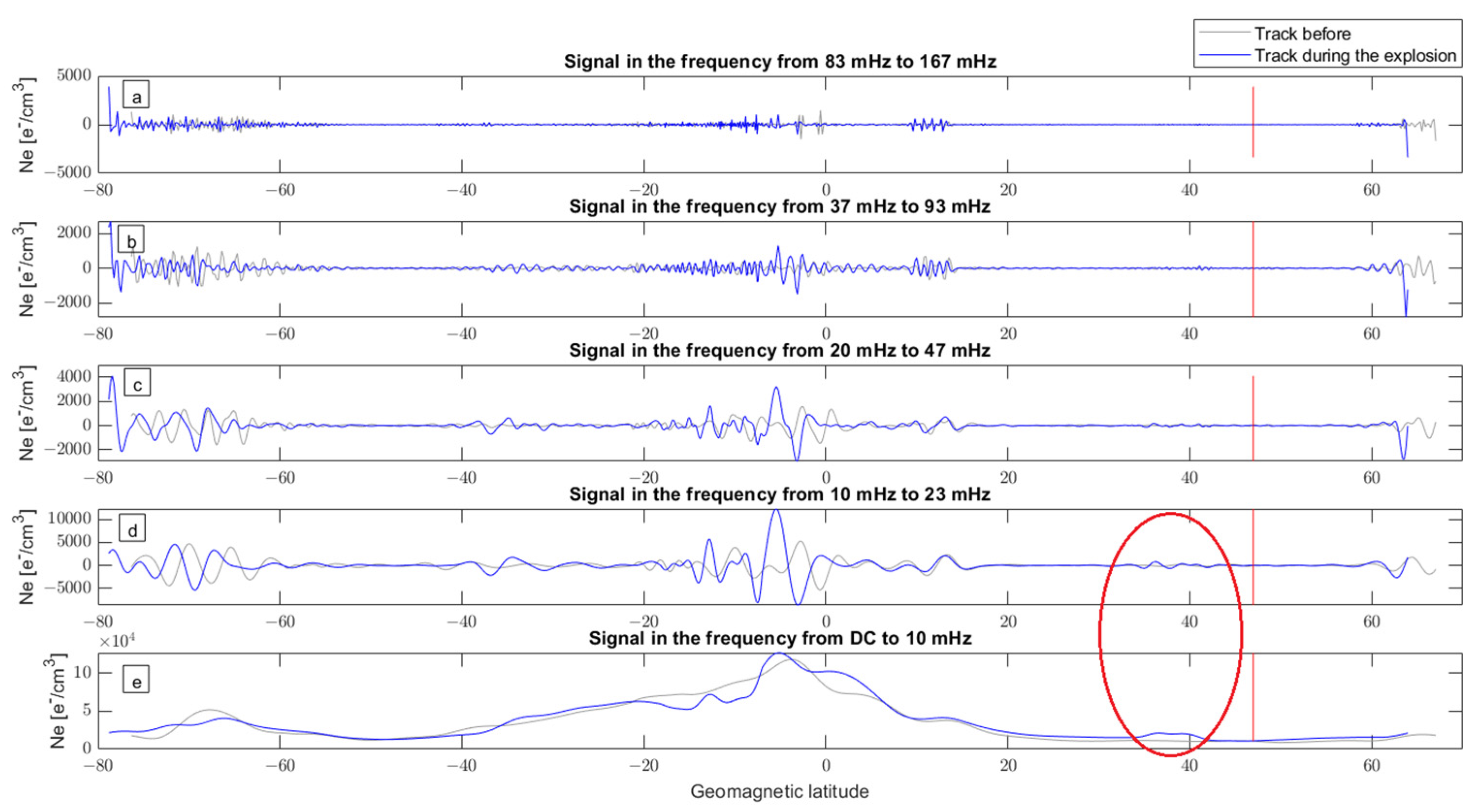
2.3. Hunga Tonga-Hunga Ha’apai Volcano Explosion Effect on the Ionosphere

On 15 January 2022, the submarine stratovolcano Hunga Tonga-Hunga Ha’Apai produced a wide explosion, estimated to have a Volcano Explosive Index (VEI) of about 6 [17]. Several studies have investigated such a large and rare geophysical event, considering that this is the first time it has been possible to monitor and observe such a geophysical event from several satellites [18,19,20]. Here, we further investigate the CSES satellite electron density measurements already presented by D’Arcangelo et al. [21]. During the volcano explosion (estimated from seismic data at 4:15:45 UTC), CSES-01 was flying westward of the volcano (see Figure 4). In order to search if the electron density profile could contain some signature of the volcano explosion, we compared the Ne profile with that of the previous track at the same local time (about 2:00 P.M.).
In particular, in Figure 5, we have decomposed the electron density latitudinal profiles in five different frequency bands from the continuum (DC) to half of the sampling frequency of 333 mHz. As the two orbits were descending, the time went from right to left. Therefore, the blue data at the left of the red vertical line (time of the explosion) were acquired after it, the blue on the right, and all the grey before it. In particular, we noted an increment of electron density and some slow oscillations (underlined by red oval) that were unique in the track after the explosion from about 44° N to 32° N, as visible in subpanels d and e of Figure 5. In the previous paper, this disturbance was underlined with a red circle and the number “1” in Figure 15 of [21]. We propose that such disturbance is the ionospheric shock induced by the explosion by electromagnetic coupling between the atmosphere/ocean (i.e., under the sea where the explosion originated) and the ionosphere. This can be explainable only by electromagnetic mechanisms due to the very short time period and the relatively far position of the satellite at the time of the explosion (overflying the Kamchatka Islands, see Figure 4).
Such a violent volcano explosion generated a pressure wave (Lamb wave) that propagated at the speed of sound all around the Earth and was globally recorded by barometric sensors [21,22,23]. In particular, the CSES-01 satellite orbit at around 10 UT passed almost tangent to the Lamb wavefront (see Figure 17 in [21]), and we provide further details of this orbit in Figure 6. We calculated a smoothed signal by a moving average window of 11 samples to remove the possible oscillation of the measurements that made it unclear whether they were due to the instrument or a real oscillation of the ionosphere. The distance of the satellite with respect to the front of the pressure wave was also calculated, taking into account that both the satellite and the front wave were moving simultaneously. The pressure wave was simplified as perfectly circular, and its speed was considered fixed at 1100 km/hour. In truth, the speed depends on air temperature and can be influenced by orography, but our calculus could be a first approximation. Finally, we calculated the correlation between the smoothed electron density and the surface atmospheric pressure provided by ECMWF ERA-5 [24]. The correlation between the two profiles is 36%, supporting the coupling between the atmosphere and the ionosphere. Even though the ionosphere electron density seems reasonably correlated (considering the distance of the geo-layers), only a part of the track could be affected by the Lamb wave that, in any case, seems to have perturbed the electron density in the ionosphere.

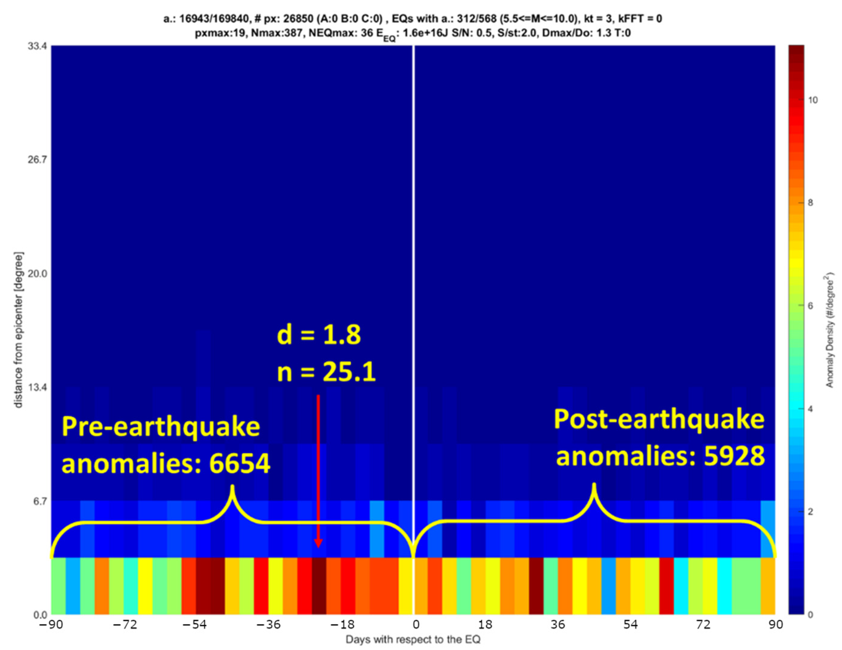
2.4. Worldwide Statistical Investigation of Ionospheric Electron Density Measured by CSES-01

A limitation of single case studies, as in the previous examples, is that some anomalies may appear before the geophysical hazard by chance but are not related to the incoming event. To address this problem, a statistical study on many events, such as the M5.5+ Worldwide earthquakes, can prove (or not) the relationship between ionospheric anomalies and earthquakes. De Santis et al. [11] and Marchetti et al. [12] provided strong evidence that not only a consistent number of M5.5+ shallow earthquakes are proceeded by Swarm magnetic and electron density anomalies, but also that the anticipation time increases with magnitude according to Rikitake’s law [10] and that the frequency of magnetic anomalies seems to depend on sea or land epicentre location. De Santis et al. [25] conducted a preliminary analysis of CSES Ne anomalies related to M5.5+ earthquakes that we extended to 24 months of data (i.e., two years).
Figure 7 shows the result of the Worldwide Statistical Correlation (WSC) algorithm (details of the methods in [11,12]) applied to CSES electron density data. The 5.5+ earthquakes were investigated in a symmetric period from 90 days before to 90 days after the 568 seismic events. We immediately note that the results present interesting features and are statistically significant. The analysis shows more pre-earthquake than post-earthquake anomalies. In addition, the absolute maximum concentration is located before the earthquakes. Despite a large number of total extracted anomalies (169,840), the statistical significance of the concentrations potentially related to the pre-earthquake process is relatively high (i.e., 1.8 higher than a random concentration as indicated by the “d” factor defined in [11,12]). Furthermore, it is notable that a significantly higher number of anomalies (6654) were located in the 90 days before the earthquakes compared to the lower number of anomalies (5928) in the 90 days following the same events. Finally, it seems that from about 56 days before the earthquakes, there is an activation of the ionosphere, showing a “swarm” of anomalies with a peak of about one month before the earthquake origin time. Future studies are necessary to further extend the analysis at 4.5 years (or more) of CSES mission data and thoroughly investigate the relationship between CSES anomalies and earthquakes with a similar approach already used for Swarm in [11,12].

3. Discussion and Conclusions

The study of ionospheric disturbances is often afforded by investigating a geophysical hazard event or by a statistical approach to a wide number of case studies. Both methodologies present advantages and disadvantages. The former permits us to thoroughly investigate what happened before the specific event by taking into account several factors, from the geomagnetic conditions to the tectonic and geological settings, while it is not able to distinguish if some alterations of the ionosphere are by chance or really related to the incoming event. A statical study such as the one we show in Figure 7 allows us to confirm whether a phenomenon is recurrent or not, but it lacks specific details. For example, we show evidence that about 20 days before 36 earthquakes, there was a significant concentration of CSES Ne anomalies 1.8 times higher than what was expected by chance. Still, the details, such as which LAIC mechanisms were involved, and whether or not a conjugate anomaly exists (as in the example shown in Figure 1), are missing. Finally, even if we confirm the existence of LAIC prior to earthquakes, future studies need to better understand the LAIC propagation mechanisms and the features that influence the LAIC, as partially done in [11,12].

Author Contributions

Conceptualisation, methodology, software, formal analysis, investigation, visualisation, writing—original draft preparation, D.M.; validation, supervision, project administration, funding acquisition, K.Z. and D.M.; data curation, D.M., R.Y., Z.Z. and X.S.; writing—review and editing, D.M., W.C., Y.C., M.F., T.W., J.W., D.Z., H.Z. and Y.Z. All authors have read and agreed to the published version of the manuscript.

Funding

This research was funded by the National Natural Science Foundation of China, grant number 41974084; the China Postdoctoral Science Foundation, grant number 2021M691190 and the International Cooperation Project of the Department of Science and Technology of Jilin Province, grant number 20200801036GH.

Institutional Review Board Statement

Not applicable.

Informed Consent Statement

Not applicable.

Data Availability Statement

Swarm data are freely available via ftp and http at swarm-diss.eo.esa.int server (last access on 27 July 2022). China Seismo Electromagnetic Satellite data are freely available at www.leos.ac.cn (last access on 15 December 2020) upon registration and approval.

Acknowledgments

We acknowledge Saioa Arquero Campuzano, Dario Sabbagh, Martina Orlando, Loredana Perrone, Rita Di Giovambattista, Giorgiana De Franceschi, Maurizio Soldani, Domenico Di Mauro, Adriano Nardi, Cristiano Fidani, Salvatore Roberto Maugeri, Alessandro Bonforte, Mauro Regi, Angelo De Santis, Serena D’Arcangelo, Gianfranco Cianchini and Alessandro Ippolito to have participated in some scientific discussions of the present work. D.M. and Z.Z. acknowledge the International Space Science Institute (ISSI at Bern, Switzerland) for supporting International Team 553 led by Essam Ghamry and Zeren Zhima.

Conflicts of Interest

The authors declare no conflict of interest. The funders had no role in the design of the study; in the collection, analyses, or interpretation of data; in the writing of the manuscript; or in the decision to publish the results.

References

  1. Mansouri Daneshvar, M.R.; Freund, F.T. Remote Sensing of Atmospheric and Ionospheric Signals Prior to the Mw 8.3 Illapel Earthquake, Chile 2015. Pure Appl. Geophys. 2017, 174, 11–45. [Google Scholar] [CrossRef]
  2. Parrot, M. Statistical Analysis of Automatically Detected Ion Density Variations Recorded by DEMETER and Their Relation to Seismic Activity. Ann. Geophys. 2012, 55, 149–155. [Google Scholar] [CrossRef]
  3. Yan, R.; Parrot, M.; Pinçon, J.-L. Statistical Study on Variations of the Ionospheric Ion Density Observed by DEMETER and Related to Seismic Activities: Ionospheric Density and Seismic Activity. J. Geophys. Res. Space Phys. 2017, 122, 12421–12429. [Google Scholar] [CrossRef]
  4. Pulinets, S.; Ouzounov, D. Lithosphere–Atmosphere–Ionosphere Coupling (LAIC) Model—An Unified Concept for Earthquake Precursors Validation. J. Asian Earth Sci. 2011, 41, 371–382. [Google Scholar] [CrossRef]
  5. Freund, F. Pre-Earthquake Signals: Underlying Physical Processes. J. Asian Earth Sci. 2011, 41, 383–400. [Google Scholar] [CrossRef]
  6. Molchanov, O.A.; Hayakawa, M. Generation of ULF Electromagnetic Emissions by Microfracturing. Geophys. Res. Lett. 1995, 22, 3091–3094. [Google Scholar] [CrossRef]
  7. Hayakawa, M.; Kasahara, Y.; Nakamura, T.; Hobara, Y.; Rozhnoi, A.; Solovieva, M.; Molchanov, O.; Korepanov, V. Atmospheric Gravity Waves as a Possible Candidate for Seismo-Ionospheric Perturbations. J. Atmos. Electr. 2011, 31, 129–140. [Google Scholar] [CrossRef]
  8. Dobrovolsky, I.P.; Zubkov, S.I.; Miachkin, V.I. Estimation of the Size of Earthquake Preparation Zones. Pure Appl. Geophys. 1979, 117, 1025–1044. [Google Scholar] [CrossRef]
  9. De Santis, A.; Marchetti, D.; Spogli, L.; Cianchini, G.; Pavón-Carrasco, F.J.; Franceschi, G.D.; Di Giovambattista, R.; Perrone, L.; Qamili, E.; Cesaroni, C.; et al. Magnetic Field and Electron Density Data Analysis from Swarm Satellites Searching for Ionospheric Effects by Great Earthquakes: 12 Case Studies from 2014 to 2016. Atmosphere 2019, 10, 371. [Google Scholar] [CrossRef]
  10. Rikitake, T. Earthquake Precursors in Japan: Precursor Time and Detectability. Tectonophysics 1987, 136, 265–282. [Google Scholar] [CrossRef]
  11. De Santis, A.; Marchetti, D.; Pavón-Carrasco, F.J.; Cianchini, G.; Perrone, L.; Abbattista, C.; Alfonsi, L.; Amoruso, L.; Campuzano, S.A.; Carbone, M.; et al. Precursory Worldwide Signatures of Earthquake Occurrences on Swarm Satellite Data. Sci. Rep. 2019, 9, 20287. [Google Scholar] [CrossRef]
  12. Marchetti, D.; De Santis, A.; Campuzano, S.A.; Zhu, K.; Soldani, M.; D’Arcangelo, S.; Orlando, M.; Wang, T.; Cianchini, G.; Di Mauro, D.; et al. Worldwide Statistical Correlation of Eight Years of Swarm Satellite Data with M5.5+ Earthquakes: New Hints about the Preseismic Phenomena from Space. Remote Sens. 2022, 14, 2649. [Google Scholar] [CrossRef]
  13. Liperovsky, V.A.; Pokhotelov, O.A.; Meister, C.-V.; Liperovskaya, E.V. Physical Models of Coupling in the Lithosphere-Atmosphere-Ionosphere System before Earthquakes. Geomagn. Aeron. 2008, 48, 795–806. [Google Scholar] [CrossRef]
  14. De Santis, A.; Cianchini, G.; Marchetti, D.; Piscini, A.; Sabbagh, D.; Perrone, L.; Campuzano, S.A.; Inan, S. A Multiparametric Approach to Study the Preparation Phase of the 2019 M7.1 Ridgecrest (California, United States) Earthquake. Front. Earth Sci. 2020, 8, 540398. [Google Scholar] [CrossRef]
  15. Marchetti, D.; De Santis, A.; Campuzano, S.A.; Soldani, M.; Piscini, A.; Sabbagh, D.; Cianchini, G.; Perrone, L.; Orlando, M. Swarm Satellite Magnetic Field Data Analysis Prior to 2019 Mw = 7.1 Ridgecrest (California, USA) Earthquake. Geosciences 2020, 10, 502. [Google Scholar] [CrossRef]
  16. Xie, T.; Chen, B.; Wu, L.; Dai, W.; Kuang, C.; Miao, Z. Detecting Seismo-Ionospheric Anomalies Possibly Associated With the 2019 Ridgecrest (California) Earthquakes by GNSS, CSES, and Swarm Observations. JGR Space Phys. 2021, 126, e2020JA028761. [Google Scholar] [CrossRef]
  17. Poli, P.; Shapiro, N.M. Rapid Characterization of Large Volcanic Eruptions: Measuring the Impulse of the Hunga Tonga Ha’apai Explosion From Teleseismic Waves. Geophys. Res. Lett. 2022, 49, e2022GL098123. [Google Scholar] [CrossRef]
  18. Heki, K. Ionospheric Signatures of Repeated Passages of Atmospheric Waves by the 2022 Jan. 15 Hunga Tonga Eruption Detected by QZSS-TEC Observations in Japan. Earth Planets Space 2022, 74, 1–12. [Google Scholar] [CrossRef]
  19. Matoza, R.S.; Fee, D.; Assink, J.D.; Iezzi, A.M.; Green, D.N.; Kim, K.; Toney, L.; Lecocq, T.; Krishnamoorthy, S.; Lalande, J.-M.; et al. Atmospheric Waves and Global Seismoacoustic Observations of the January 2022 Hunga Eruption, Tonga. Science 2022, 377, 95–100. [Google Scholar] [CrossRef]
  20. Yuen, D.A.; Scruggs, M.A.; Spera, F.J.; Zheng, Y.; Hu, H.; McNutt, S.R.; Thompson, G.; Mandli, K.; Keller, B.R.; Wei, S.S.; et al. Under the Surface: Pressure-Induced Planetary-Scale Waves, Volcanic Lightning, and Gaseous Clouds Caused by the Submarine Eruption of Hunga Tonga-Hunga Ha’apai Volcano. Earthq. Res. Adv. 2022, 2, 100134. [Google Scholar] [CrossRef]
  21. D’Arcangelo, S.; Bonforte, A.; De Santis, A.; Maugeri, S.R.; Perrone, L.; Soldani, M.; Arena, G.; Brogi, F.; Calcara, M.; Campuzano, S.A.; et al. A Multi-Parametric and Multi-Layer Study to Investigate the Largest 2022 Hunga Tonga–Hunga Ha’apai Eruptions. Remote Sens. 2022, 14, 3649. [Google Scholar] [CrossRef]
  22. Amores, A.; Monserrat, S.; Marcos, M.; Argüeso, D.; Villalonga, J.; Jordà, G.; Gomis, D. Numerical Simulation of Atmospheric Lamb Waves Generated by the 2022 Hunga-Tonga Volcanic Eruption. Geophys. Res. Lett. 2022, 49, e2022GL098240. [Google Scholar] [CrossRef]
  23. Lin, J.; Rajesh, P.K.; Lin, C.C.H.; Chou, M.; Liu, J.; Yue, J.; Hsiao, T.; Tsai, H.; Chao, H.; Kung, M. Rapid Conjugate Appearance of the Giant Ionospheric Lamb Wave Signatures in the Northern Hemisphere After Hunga-Tonga Volcano Eruptions. Geophys. Res. Lett. 2022, 49, e2022GL098222. [Google Scholar] [CrossRef]
  24. Hersbach, H.; Bell, B.; Berrisford, P.; Hirahara, S.; Horányi, A.; Muñoz-Sabater, J.; Nicolas, J.; Peubey, C.; Radu, R.; Schepers, D.; et al. The ERA5 Global Reanalysis. Q. J. R. Meteorol. Soc. 2020, 146, 1999–2049. [Google Scholar] [CrossRef]
  25. De Santis, A.; Marchetti, D.; Perrone, L.; Campuzano, S.A.; Cianchini, G. Statistical Correlation Analysis of Strong Earthquakes and Ionospheric Electron Density Anomalies as Observed by CSES-01. Il Nuovo Cim. C 2021, 44, 1–4. [Google Scholar] [CrossRef]
Figure 1. Swarm Alpha magnetic field residual, track 9 on 2 January 2015, i.e., 258 days before M8.3 Illapel (Chile) 2015 earthquake. The 3° latitude anomalous (kt = 2.5) windows are marked by red colour. The map of the region is represented with a yellow circle that shows the Dobrovolsky area of the earthquake, whose epicentre is marked with a green star and the satellite track projection by a brown line. The title indicates which satellite is represented (A = Alpha, B = Bravo, C = Charlie), the date of acquisition, track number, the direction of flying (U = Upward, D = Downward), local time (meanLT) and universal time (meanUT) at the middle of the plotted track. Geomagnetic indexes Dst and ap at acquisition time as also reported.
Proceedings 87 00034 g001
Figure 2. Tracks 11 (blue colour) and 13 (green colour) following Figure 1. As in Figure 1, the anomalies are marked by red lines, and the representation and the title information are the same of Figure 1. Track 13 has no “red” anomaly as it is outside the Dobrovolsky area and the code automatically excludes it.
Proceedings 87 00034 g002
Figure 3. Increase of electron density about one month before Mw = 7.1 Ridgecrest (California, US) 6 July 2019 earthquake. Electron Density (Ne) data are from Swarm Alpha (black) and CSES-01 (blue) satellites. The map and the title information are the same as in Figure 1.
Proceedings 87 00034 g003
Figure 4. Map with start and end UT times of CSES-01 satellite in the track before (grey) and during (blue) the explosion of Hunga Tonga-Hunga Ha’apai volcano, represented as a red triangle. The satellite’s position at the time of the explosion is marked with a red cross. Both tracks are in descending (daytime) directions as indicated by the black arrows.
Proceedings 87 00034 g004
Figure 5. Frequency investigation of the electron density profile of CSES acquired during the Hunga Tonga Hunga Ha’Apai volcano eruption of 15 January 2022 at 4:15:45 UTC. The blue and grey lines represent the signal acquired in the daytime orbits during and before the explosion, respectively. The signal has been decomposed into five frequency bands: (a) from 83 mHz to 167 mHz; (b) from 37 mHz to 93 mHz; (c) from 20 mHz to 47 mHz; (d) from 10 mHz to 23 mHz; (e) from DC to 10 mHz. The vertical red line represents the position of the CSES satellite at the eruption time. Both tracks are descending. The red circle underlines the particular signal recorded by CSES just after the eruption may be induced by the volcano explosion.
Proceedings 87 00034 g005
Figure 6. Detailed investigation of the electron density profile of the CSES-01 satellite likely affected by the ionospheric effect of the Lamb wave produced by the Hunga Tonga-Hunga Ha’apai volcano explosion of 15 January 2022.
Proceedings 87 00034 g006
Figure 7. WSC algorithm applied to CSES Ne anomalies (recorded in April, August and September 2018, in 2019 and from January to September 2020) correlated with M5.5+ earthquakes from 90 days before until 90 days after the event. The number of anomalies in the first row before and after the earthquakes is also reported. Two statistical parameters for the maximum anomaly concentration, “d” and “n”, are reported. “d” represents how many times higher the concentration was than the average random one and n represents by how many standard deviations of random simulation such concentration is higher (full definition and details in [11,12]).
Proceedings 87 00034 g007
Disclaimer/Publisher’s Note: The statements, opinions and data contained in all publications are solely those of the individual author(s) and contributor(s) and not of MDPI and/or the editor(s). MDPI and/or the editor(s) disclaim responsibility for any injury to people or property resulting from any ideas, methods, instructions or products referred to in the content.

