

Unmanned Aerial Vehicle 3D Path Planning Based on an Improved Artificial Fish Swarm Algorithm


1
State Key Laboratory of Public Big Data, Guizhou University, Guiyang 550025, China
2
College of Mechanical Engineering, Guizhou University, Guiyang 550025, China
*
Author to whom correspondence should be addressed.
Drones 2023, 7(10), 636; https://doi.org/10.3390/drones7100636
Submission received: 28 August 2023
/
Revised: 10 October 2023
/
Accepted: 11 October 2023
/
Published: 16 October 2023
(This article belongs to the Special Issue Drones Navigation and Orientation)
Abstract
:A well-organized path can assist unmanned aerial vehicles (UAVs) in performing tasks efficiently. The artificial fish swarm algorithm (AFSA) is a widely used intelligent optimization algorithm. However, the traditional AFSA exhibits issues of non-uniform population distribution and susceptibility to local optimization. Despite the numerous AFSA variants introduced in recent years, many of them still grapple with challenges like slow convergence rates. To tackle the UAV path planning problem more effectively, we present an improved AFSA algorithm (IAFSA), which is primarily rooted in the following considerations: (1) The prevailing AFSA variants have not entirely resolved concerns related to population distribution disparities and a predisposition for local optimization. (2) Recognizing the specific demands of the UAV path planning problem, an algorithm that can combine global search capabilities with swift convergence becomes imperative. To evaluate the performance of IAFSA, it was tested on 10 constrained benchmark functions from CEC2020; the effectiveness of the proposed strategy is verified on the UAV 3D path planning problem; and comparative algorithmic experiments of IAFSA are conducted in different maps. The results of the comparison experiments show that IAFSA has high global convergence ability and speed.
1. Introduction
UAVs have received significant attention and utilization in both civilian and military domains [1]. UAVs are autonomous or remotely controlled aircrafts that offer numerous advantages over manned aircraft, including cost-effectiveness, flexibility, and the ability to operate in challenging or hazardous environments. In the civilian sector, UAVs have revolutionized various fields, such as agricultural crop protection [2,3], aerial photography [4], express transportation [5,6], and ocean remote sensing [7]. In the military sector, they have become vital assets for intelligence gathering [8], reconnaissance surveillance [9], and other complex and dangerous missions. The role of UAVs in the delivery of essential supplies during seismic disaster relief operations in mountainous areas is of particular interest. Mountainous regions often involve challenges such as complex geological conditions and limited transportation options, which impede traditional supply/delivery methods. UAVs, with their speed and agility, can effectively transport relief materials to disaster-stricken areas, providing crucial support for rescue operations [10].
One fundamental requirement for a UAV to effectively accomplish its intended mission is effective path planning [11]. The path planning problem for UAVs involves generating a collision-free trajectory from the starting point to the target point that accounts for the given flight conditions and environmental constraints. The planned path should minimize the cost and comply with the relevant constraints. Due to the complexity of optimization problems with multiple constraints, traditional optimization strategies often face challenges in finding the best solution [12].
Sampling-oriented path planning algorithms have been widely studied and applied because of their low computational complexity when solving complex, high-dimensional problems. Tan Liguo uses the RRT algorithm to extend the node to address the time consumption and low success rate of UAV path planning in complex blockage environments [13]. The path planning solutions of RRT have better adaptability than traditional strategies, allowing them to cope with obstacle changes in dynamic environments and find feasible paths more quickly [14,15], but these methods may run indefinitely when paths do not exist.
In contrast, nature-inspired optimization algorithms offer distinct advantages when addressing intricate optimization problems like path planning. Unlike traditional gradient-based algorithms, natural heuristic algorithms do not rely on the gradient information of the objective function but search by directly evaluating the objective function values. These algorithms are not constrained by mathematical conditions such as continuous differentiability and can be applied to discrete optimization problems such as integer programming [16]. Even in nonlinear control systems, natural heuristic algorithms are effective for parameter estimation and control optimization [17,18]. Notable examples of these common heuristic algorithms encompass particle swarm optimization (PSO) [19,20,21], ant colony optimization (ACO) [22,23], artificial bee colony (ABC) [24,25,26], the genetic algorithm (GA) [27,28,29], beetle antennae search algorithm (BAS) [16], and Harris hawks optimization (HHO) [30], among others. Ref. [31] proposes a novel path planning approach integrating Voronoi diagram generation and Dijkstra’s shortest path algorithm, introducing an efficient PSO metaheuristic algorithm that improves solution quality compared to traditional PSO by simulating real-world scenarios, with enhancements ranging from 5% to 22% under different wind conditions. Ref. [32] explores the impact of common U-shaped obstacles in 3D space on path planning for UAVs and presents a self-heuristic ACO-based method. This method defines the entire space by constructing a grid workspace model and designing two different search strategies for selecting the next path node to avoid ACO algorithm deadlock, effectively addressing the path planning problem for UAVs encountering U-shaped obstacles in 3D space. Ref. [25] proposes an improved ABC algorithm based on multi-strategy synthesis for UAV path planning in complex urban environments and provides rapid and optimal paths. A feasible approach was proposed in [33] to solve the real-time path planning problem for UAVs, which meets the requirements of flight safety and improves the efficiency of path planning, especially in dynamic obstacle avoidance.
The methods proposed in the above literature include problems such as unrealistic map settings, ease of falling into local optimums, and unreasonable path optimization. Notably, the artificial fish swarm algorithm (AFSA) in the population intelligence algorithm is widely used for optimization because of its flexibility, insensitivity to initial parameter settings, and global search capability [34]. It stimulates the preying, following, and swarming behaviors of fish, utilizing multiple fish to collaboratively search and optimize functions or solve problems. Within AFSA, each fish makes various behavioral decisions based on the objective function information within their field of vision. Different fish interact through information exchange to achieve synergy, ultimately leading the fish population toward the optimal state. In comparison to the BAS algorithm, AFSA offers greater flexibility in adjusting search step lengths and striking a balance between local and global search through various behaviors. BAS, on the other hand, relies more on antenna length parameters. In contrast to HHO, AFSA features autonomous individuals within the fish population and lacks a distinct tracking-evading relationship, which helps prevent falling into local optima. In the context of the problem at hand, AFSA achieves collaborative search through information dissemination, while PSO depends on velocity to maintain search direction. The local interactions within AFSA can provide richer search information. Ref. [35] proposed incorporating directional operators and probabilistic weighting factors to enhance the path quality of autonomous surface vessels (ASVs). Ref. [36] addresses the path planning problem of ASVs under complete constraints by employing a cost expansion strategy. Ref. [37] introduces a novel approach combining an artificial fish school algorithm with continuous segmented Bessel curves to generate low-precision, high-quality paths with minimal inflection points and reduced length for robots.
However, relatively few reports discuss applying AFSAs to the path planning problem of UAV 3D environments. By analyzing and organizing the above literature, an improved artificial fish swarming algorithm (IAFSA) is proposed to address this problem and obtain the optimal path more effectively than other algorithms. The following are the contributions to this paper:
- A multi-strategy fusion IAFSA is proposed to improve the original AFSA. Specifically, the refractive opposition learning (ROL) strategy is introduced to address the issue of the uneven distribution of the fish swarm. Then, the adaptive spiral strategy (ASS) is employed to balance the trade-off between exploration and exploitation of the algorithm. Finally, the adaptive elimination and regeneration (AER) mechanism is implemented to effectively prevent the algorithm from converging to local optima. Through the integration of these strategies, the improved algorithm achieves superior performance compared to the original AFSA.
- Experiments on the effectiveness of the strategy are performed for the UAV path planning issue, and the experimental results are analyzed. Then, the suggested algorithm is compared with itself in maps of different complexity to explore the effect of the algorithm.
This manuscript is structured as follows: Section 2 describes the problem of UAV path planning. Section 3 introduces the standard AFSA, the proposed optimization idea, and the improvement method of the IAFSA. Section 4 presents the validation experiment, the strategy effectiveness experiment, and the algorithm comparison experiment on the test function. Section 5 presents the conclusions.
2. Problem Description for Path Planning
In this section, a mountainous environment model for UAVs is established, along with a corresponding UAV path planning model. A dual-objective model is formulated that accounts for both the minimization of UAV path length and the optimization of flight energy consumption. Additionally, trajectory optimization methods for UAVs are introduced.
2.1. 3D Scene Setting
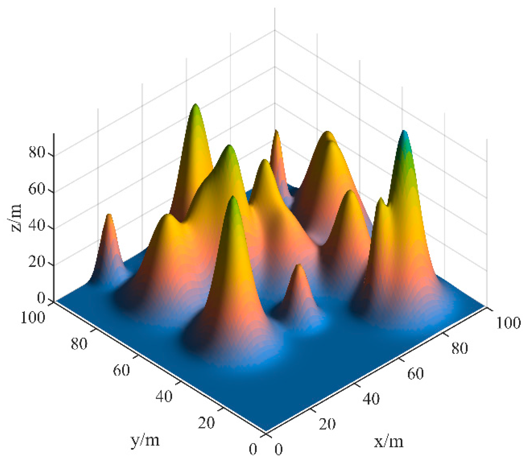
UAVs often operate in complex terrains in practical scenarios such as coastal search and disaster relief. The terrain model serves as a fundamental basis for UAV path planning. To better simulate real-world conditions, the complex 3D terrain can be described using the following exponential (1) function [39]:
The coordinates are utilized to represent the position in the two-dimensional plane. denotes the number of generated peaks, where correspond to the height control parameter and central coordinates of the respective peak. represents the rate of change in the peak along the -axis, while denotes the rate of change along the -axis. Additionally, denotes the exponential function.
This formulation enables multiple peaks to be created and manipulated within the given plane. The parameters , , , , and collectively contribute to the diverse and intricate landscape generated by the peaks.
Based on the model (1) formulation, ten randomly generated peaks were created within a 3D space of dimensions , as illustrated in Figure 1.
2.2. Establishment of the Multiobjective Fitness Function
Let the coordinates of the starting point in the aforementioned complex 3D environment be and the coordinates of the destination point be . The coordinates of the intermediate node are denoted as , where .
The objective function is to minimize the cost of the drone’s travel and energy consumption while executing the mission. Assuming that the total cost of completing a single mission by the drone is , the following equation is obtained.
where represent the cost of travel and energy consumption, respectively. and denote the weights assigned to these costs and satisfy the condition .
2.2.1. Cost of Travel
The flight distance covered by a UAV while completing each mission is determined by summing the Euclidean distances between adjacent path nodes, denoted as . The UAV departs from the starting point , passes through node , and reaches the destination point , with the expression of the cost of flight distance denoted as .
Equation (3) can be reformulated as follows:
2.2.2. Energy Consumption
Under constant velocity, power is primarily proportional to weight. Weight consists of three main components: airframe, battery, and payload. Therefore, increasing payload increases the overall weight of the aircraft, resulting in higher power consumption. Energy consumption is a crucial factor that limits the performance of UAVs as different behaviors of the aircraft result in differing amounts of power consumption. If the payload influence is not accounted for, the planned flight path may not be achievable in practical missions. Hence, an effective payload penalty coefficient, denoted as , is introduced.
According to research conducted by Song et al. [40], the flight time and energy consumption of UAVs increase linearly with the mass of the loaded product. Therefore, the effective payload penalty coefficient for logistics UAVs during delivery missions is assumed to be directly proportional to the payload quantity . represents the maximum payload capacity of the logistics UAVs, while represents the maximum value of the effective payload penalty coefficient.
Then, the effective payload penalty coefficient is expressed as follows:
The energy cost can be described as follows:
where and indicate the energy spent by UAVs during horizontal and vertical flight, respectively. The number represents the energy consumption per unit distance for horizontal flight. denotes the energy consumption generated per unit distance for vertical height. It is worth noting that in this model, a simplification of the same power consumption for ascent and descent has been made for the sake of reserving safe power.
2.3. Restrictions and Path Smoothing
To guarantee that the UAV’s flight route remains within the defined airspace, the following constraints must be satisfied:
where is the restricted space range.
In drone path planning, it is common to impose navigation angle constraints on unmanned aerial vehicles to restrict their flight direction and orientation [41,42,43].
The current position of the UAV is , and under the condition , the UAV following the turning angle can be described by Equation (10). In Equation (11), is the climb angle of the current position.
where is the maximum angle of turning, and is the maximum climb angle.
The use of mathematical expression constraints in UAV path planning poses significant challenges. These constraints make it challenging to precisely describe complex paths, often resulting in path discontinuities and a lack of smoothness. Simultaneously satisfying various constraints becomes a complex task, ultimately restricting path choices and hindering optimization. In contrast, spline curve methods offer a more optimized, smoother, and continuous approach to path planning. Spline curves reduce UAV vibrations and bumps, enhancing comfort and stability. They also provide a better simulation of natural curves, ensuring path harmonization. Utilizing optimization algorithms, these methods can efficiently identify optimal paths within specified constraints, significantly improving efficiency.
Spline Function Definition: Given an existing function , which satisfies a third-degree polynomial definition within each interval , where . The function is referred to as a spline function with nodes . If at the node , there exists an equation and the equation holds true throughout, then is termed a spline interpolation function.
In each subinterval satisfying the following:
where are the coefficient to be determined.
Faction has second-order continuous derivatives in the interval and thus satisfies at the nodes.
The boundary condition can be described as follows:
3. Algorithm Description
In the previous section, we built a 3D environment and established a fitness function that considers UAV path planning. We also proposed using spline interpolation to generate a smooth path. Among these, the process points between the start and end points are especially important, because the process points directly affect the final path quality. In order to obtain optimized process points, this section will introduce an IAFSA.
In this section, an overview of the traditional AFSA is provided, followed by a discussion on the four key improvements made in the IAFSA for UAV trajectory planning. The improvements include generating the initial population using an ROL strategy, enhancing convergence speed through adaptive spiral vision, incorporating social experience locations to reinforce following behavior, and implementing population regeneration to avoid local optima. Finally, the specific implementation steps of the IAFSA for UAV path planning are presented.
3.1. Traditional AFSA
The AFSA is a population intelligence algorithm that seeks optimization by imitating the feeding behavior of fish in a specified search area space. The AFSA uses a local-to-whole optimization approach. First, each artificial fish in a group of artificial fish performs a local optimization search and information transfer according to a set perceptual range and behavioral mechanism. Then, the overall optimization is achieved based on the distribution of fish locations.
In a school of fish, represents the state of the fish, and denotes the dimension of each individual. denotes the current food concentration, and two-norm represents the distance between two fish.
The AFSA consists of four main behaviors: prey behavior, swarming behavior, following behavior, and random behavior. Figure 2 shows the main behavioral mechanisms of a traditional AFSA. These behaviors are specifically described as follows:
3.1.1. Preying Behavior
In the traditional AFSA algorithm, the artificial fish randomly chooses a position within the visual range based on the current position . If the food concentration , the artificial fish moves one step size toward . Otherwise, it randomly chooses another position to compare the food concentration. After exploring for the maximum number of preying attempts times, if the conditions for advancement are not met, a random step is taken.
The position can be defined as (16) and provides a random position state in the visual range next to the current fish.
The fish moves toward if the food concentration . This is accomplished by the following:
3.1.2. Following Behavior
In the field of view, position corresponds to the food concentration , and the state of the position satisfies . This indicates that a fish in the school finds a better position, assuming that there are artificial fish in the field of view where , indicating that the position is not crowded. then moves toward (18).
The AFSA will engage in prey behavior if no neighbors are located in the field of view or the requirements are not met.
3.1.3. Swarming Behavior
The behavior of the artificial fish mimics the natural aggregation patterns observed in real fish, where they strive to move toward a central location during each iteration. This movement strategy enables artificial fish to concentrate in areas with high food density, facilitating efficient local exploitation. One method used to determine the central location is illustrated in Equation (19):
The artificial fish moves toward the central position as expressed in (20) if the food concentration and .
Otherwise, the artificial fish executes prey behavior.
3.1.4. Random Behavior
To mitigate the risk of becoming trapped in local optima, the artificial fish adopts a random behavior when it is unable to execute other predefined behaviors. This random behavior involves the artificial fish randomly selecting a state or position within its visual field and then swimming toward the chosen location. This procedure can be expressed as follows:
3.2. Improved AFSA
3.2.1. ROL Initialization Strategy
In the context of UAV path planning, finding the globally optimal path faces challenges in complex environments. During the early stages of algorithm evolution, exploration takes precedence over exploitation, as global exploration of the search space helps prevent premature convergence or becoming trapped in local optima. Therefore, to address this issue, the ROL strategy was introduced, aiming to expand the search range and prevent the algorithm from prematurely converging to local optima.
The ROL strategy is a mathematical idea inspired by the natural phenomenon of light deflection in the propagation direction due to different refractive indices in two media [44,45]. In the analogy between ray refraction and path planning, both involve the process of finding the optimal path in a target space. During light propagation, refraction occurs when interfaces with different refractive indices are encountered, thus changing the direction of propagation. Similarly, in path planning, when a better path is found, the path direction needs to be adjusted in time. The “refraction effect” occurs when an unobstructed region of space exists when generating the initial school of fish. This effect refracts the initial set of points as a target into a new set of points, ensuring correlation between the old and new sets of points. In contrast, randomized methods do not ensure this correlation because the new points may not be correlated at all. This helps avoid revisiting previously explored regions and extends the path to unexplored regions. This ensures that a more evenly distributed initial population of fish is generated, thus improving the performance of the algorithm.
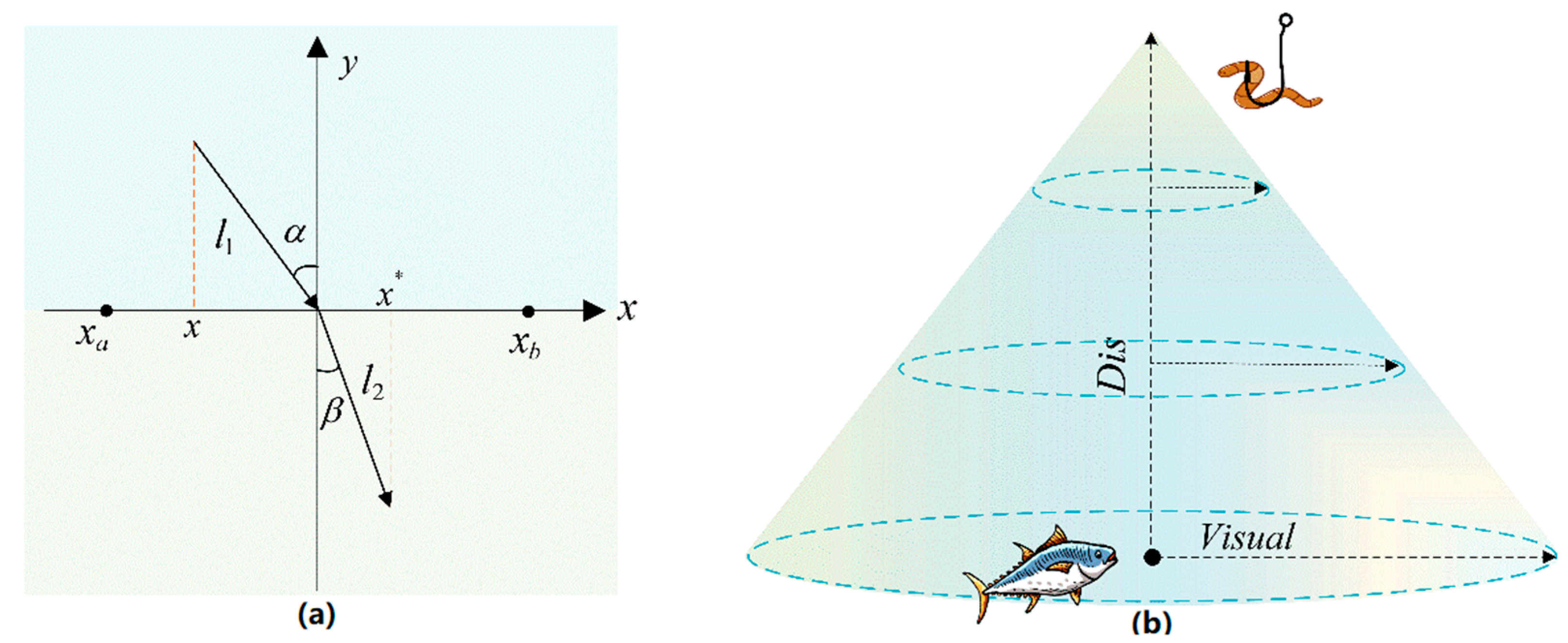
An optimization method is used to retain the more adaptive individual from the current set of solutions and from the set of opposing solutions. The concept of the ROL initialization strategy is illustrated in Figure 3a.
In Figure 3a, the -axis depicts the division between two distinct media, while the -axis represents the normal direction perpendicular to the -axis. The search range is denoted as , and the angles of incidence and refraction are represented by and , respectively, while and denote the lengths of the incident and refracted light, respectively. The point symbolizes a position within the incident region , while denotes the position of point after refraction. The lines depicted in Figure 3a illustrate the following geometric relationships:
Equation (24) defines the refraction rate .
Given , combining (24), we obtain the following, as shown in (25):
By taking in the general case and modifying Equation (25) to address the D-dimensional space problem, we obtain the following:
where is the position of the dimension of the individual. is refracted by through the refractive opposition method.
In the initialization process of the algorithm, the generated initial population is considered the incident light, and the population after refraction, where is the population size. The composition of the initial population can be expressed by (27):
The fitness of and is calculated to filter out the iterative population with high fitness, thereby improving global search ability and population diversity.
3.2.2. ASS Strategy
In UAV path planning, the path needs to be quickly adjusted in complex and dynamic environments. The IAFSA simulates the intelligent behaviors of fish in different environments, enabling dynamic path adjustments to suit various scenarios.
In this subsection, the ASS strategy is introduced to enhances the algorithm’s adaptability and improve the convergence speed and accuracy of the AFSA. This strategy adopts a spiral-shaped search path, which gradually decreases the step size in the search process and helps to approach the optimal solution quickly. This strategy has a large field of view in the initial search phase, and the field of view gradually decreases as the search proceeds striking a balance between global optimality and real-time responsiveness.
The ASS strategy is unique because it combines the characteristics of randomness and determinism, thus maintaining diversity in the search process. It can not only perform an accurate local search but also step out of local optimal solutions and search in the direction of the global optimal solution. Figure 3b shows a schematic diagram of the spiral field of the visual range. Figure 4a illustrates the preying behavior of the spiral field of the ASS strategy.
The ellipse in Figure 4a indicate that the range of an individual’s visual field varies in a spiral pattern. In the early stage of the algorithm, the range of field of view is larger, which is favorable for global search; in the later stage, the range of field of view gradually decreases, which is favorable for local fine search, and as the number of iterations increases, the range of the field of view and the step size of the fish individuals will gradually decrease when they are close to the local optimal solution. This realizes the adaptive transformation from global to local. In Figure 4b, the traditional AFSA fish will move directly toward the position closest to the food in the field of view. In IAFSA, the effect of the current global optimal solution (social experience position) is introduced while moving toward the optimal position in the field of view. The fish will move in the direction of the synthesis of the optimal position in the field of view and the socio-experiential position. This increases the ability to utilize global information.
represents the distance from the current artificial fish to the global optimum , and the value of the global optimum decreases as the exploration deepens. It is worth noting that the global optimal mentioned here refers to the optimal algorithm within the explored solution space, not the absolute optimal mathematical solution. is the spiral-shaped parameter, is the random number between , and is the initial field of view value.
3.2.3. Behavioral Enhancement
In the original pursuit behavior, the pursuit relied solely on the information of artificial fish within its visual range. However, when the visual range is limited, the artificial fish are prone to becoming trapped in local optima. In contrast, incorporating the social experience location broadens the search range, facilitating global exploration for the fish swarm. The social experience position refers to the potential global optimal solutions in the current number of iterations. These positions are selected based on the number of iterations of the algorithm and the current search state, one position at a time.
Compared to local information within the visual range, social experience offers comprehensive spatial distribution information. Therefore, by incorporating social experience positions into the pursuit behavior and integrating local and global information, fine-grained and broad-scale searches are combined.
Additionally, introducing moderate random perturbations enhances exploratory behavior, effectively improving the algorithm’s capability for global optimization. This modification adapts to the optimization needs of complex multimodal problems better than the original pursuit behavior that relied solely on local information. The enhanced following behavior is shown in Figure 4b.
The updated equation for the improved pursuit behavior’s position update is as follows:
where denotes the adaptive step factor.
3.2.4. AER Mechanism
In UAV planning, aiming for a global optimal path instead of a local one is essential, but achieving a globally optimal path search in complex environments is notably challenging.
During the search process, the mechanism randomly updates individual positions, preserving differentiation among individuals in the fish population. This approach prevents the algorithm from prematurely converging to a specific local optimum, enabling a balanced exploration of the entire search space. Maintaining diversity allows the algorithm to adapt better to complex problems and diverse environments, thereby improving global search effectiveness.
Specifically, this mechanism is triggered when the algorithm reaches a threshold value of iterations being trapped in local optima during the optimization process. The total number of individuals to be replaced is calculated according to Equation (32).
Here, the operation is used to round a number to the nearest integer. represents the current iteration count, and represents two positive real numbers. These parameters determine the proportions for updating the population.
Using the logistic mapping method shown in Equation (33), a random number sequence between is generated and mapped to integers in the range , where represents the population size, to determine which populations will be replaced.
represents the initial value.
The population is updated with the new generation using Equation (34).
where denotes the position of the individual, while denotes the updated position of the population. The random operator is generated using the t-distribution, and the global best value is denoted as .
3.2.5. IAFSA Implementation in UAV Path Planning
The previous section introduced the UAV route planning issue and the improvement strategy of IAFSA. This section discusses how to tackle the path planning problem using IAFSA in conjunction with the spline curve approach. To be more specific, the path comprises a series of interpolation points and control points, forming an ordered spline curve. The sequence starts from the initial point, followed by interpolation points, then control points, followed by interpolation points, then control points, and finally ends with interpolation points. These control points are determined through an iterative optimization process of the algorithm. The following is the specific interpolation process for generating a path:
- Use IAFSA to obtain interpolating nodes , and the sequence is given as an equivalent sequence .
- Split the coordinates of the M interpolated points into three sequences , ,
- Find the coordinate set and set , and calculate the corresponding spline interpolation function , , and .
- Calculate the corresponding values of , , and on to achieve values , , .
- is the desired path.
In the algorithm implementation, individual fish are defined with attributes, including position, path, and fitness. Position represents the location information of control points, and the initial positions are selected through the ROL strategy. Path represents the candidate path, which is obtained through the methods described above. Fitness indicates the fitness value, and once the path is obtained, we calculate the fitness value for each fish based on the objective function and accordingly update their fitness. The detailed steps of the algorithm are as follows:
- 1
- Given the initial position and the end position, generate the complex landscape map.
- 2
- Set the initialization parameters, including the number of fish , the initialization factor , the initial field of view , the adaptive step factor , the maximum number of preying tries , the crowding factor , and the maximum number of iterations .
- 3
- Randomly generate the artificial fish population according to Equation (26) to generate the opposing population , where represents the location information. Calculate the fitness value of each artificial fish corresponding to the path, filter the iterative population , and update the global optimal position .
- 4
- Calculate the field of view of the spiral search using Equation (28), with determined by Equation (31).
- 5
- Execute the swarming behavior; select each artificial fish in turn, and determine the number of artificial fish within the current artificial fish field of view and find the central location . Determine whether the location is crowded. If it is not crowded according to Equation (20), move one step toward ; otherwise, execute preying behavior.
- 6
- Perform the following behavior; determine the social experience position and the local optimal position . Determine whether the position is crowded. If it is not crowded according to Equation (30), update the current position; otherwise, perform foraging behavior.
- 7
- Compare the swarming behavior with the following behavior: update the optimal position, and obtain the target path.
- 8
- Determine whether collision occurs with the mountain. If collision occurs, expand the fitness value appropriately.
- 9
- Determine whether the population regeneration threshold is reached. If not, reach the threshold by Formulas (32)–(34) to update the population, and continue from step 4; otherwise, continue to execute steps 4–8 until the maximum number of iterations pass. End the iterations to find the optimal path.
- 10
- The IAFSA pseudocode is shown in Algorithm A1, Appendix A.
3.2.6. Time Complexity
The time complexity of this algorithm primarily consists of two main components: the ROL initialization strategy and the original AFSA. As previously explained, represents the population size, denotes the number of decision variables in the problem being solved, and represents the maximum number of algorithm iterations.
In the ROL initialization strategy, an opposing population is generated for the original population, and the individuals with the lowest fitness values are selected as the initial population. The time complexity of the initialization process comprises two parts: computing fitness values and sorting the population. Therefore, the time complexity of the initialization process can be expressed as .
The time complexity of the original AFSA mainly consists of three parts: the move step, the neighborhood search, and the fitness evaluation. In one iteration, both the moving step and the neighborhood search have a worst-case time complexity of , while the fitness evaluation has a time complexity of . Therefore, the time complexity of the original AFSA can be calculated as .
In summary, the time complexity of this algorithm is .
4. Experimental Results and Analysis
In this section, the effectiveness of the proposed IAFSA algorithm is evaluated using the 10 benchmark functions in CEC2020. The strategy effectiveness of the algorithm is also evaluated. In addition, the proposed model is simulated using the improved algorithm; for comprehensive analysis and validation, this algorithm is compared with various other algorithms based on the experimental results.
4.1. CEC2020 Experiments
The newest and most challenging numerical optimization contest, the CEC2020 benchmark function (see Table 1), was chosen for evaluating the performance of the IAFSA. This choice allows the capabilities of the proposed algorithm to be further observed. The benchmark test consists of 10 different functions categorized into single-mode, multimode, hybrid and combinatorial functions.
Numerical experiments were performed under conditions, and the proposed algorithm was compared with the original AFSA, PSO, IAFSA1 with probability weighting factors, IASA2 with integrated survey behavior, and IAFSA3 with an initialization strategy and adaptive strategy [47]. The experiments were conducted under the same conditions to attempt to provide a fair and reliable assessment of the performance of the algorithms. The experiments were conducted in a controlled environment using MATLAB 2021b on a Windows 10 operating system with an Intel(R) Core(TM) i9-12500H @ 3.1 GHz CPU and 16 GB RAM
The experimental parameters were set as follows: the number of populations was , the number of iterations was , the inertia weight of the PSO was set to , the social and cognitive weights were set to , and the particle velocity was set to . The following are IAFSA parameter settings: the factor , initial field of view , adaptive step factor , maximum number of preying tries , crowding factor , and spiral-shaped parameter . The main simulation parameters of AFSA were set as follows: ; the field of view ; the maximum number of prey trials ; and the crowding factor was set to . The other comparison algorithms were set to the same level as that of the AFSA, and the parameter settings were kept the same as those of the AFSA. Figure 5 shows the convergence curve on CEC2020. Table 2 reflects the experimental results of 30 iterations.
4.2. Strategy Validity Experiments
To assess the potential proposed strategy enhancement on the effectiveness of the AFSA in 3D path planning problems, a systematic investigation was conducted by selectively retaining specific improvement strategies or mechanisms. The aim of this investigation was to evaluate the impact of the retained strategies on the overall path planning effectiveness and to ascertain the individual contributions and significance of each component within the IAFSA framework.
The following IAFSA variations were considered for evaluation:
- IAFSA_S1: Exclusively employing the ROL initialization strategy.
- IAFSA_S2: Exclusively employing the ASS strategy.
- IAFSA_S3: Incorporating the behavioral reinforcement mechanism.
- IAFSA_S4: Implementing the AER mechanisms.
To obtain fair experimental results, the common parameters were set to be consistent across the variations: the start point coordinates were ; the end point coordinates were ; the number of populations was ; the maximum number of iterations was ; the initial field of view range was ; the maximum number of preying trials was ; and the crowding degree factor was . The adaptive step factor of IAFSA was . The spiral-shaped parameter was . The inertia weight of the particle swarm algorithm was ; the social weight and the cognitive weight were ; and the particle velocity was .
Figure 6 illustrates the comparative effectiveness of the proposed improvement strategy. The introduced strategies exhibit varying degrees of enhancement on the original algorithm. Among these variations, the IAFSA method, which combines each strategy, demonstrates the highest convergence speed and the strongest global search capability. The data on the longest path, shortest path, average path length, and standard deviation after employing the specified parameters and conducting 20 independent experiments are tabulated in Table 3.
The performance of the AFSA and the four improved schemes is compared using the data described in Table 3. The AFSA exhibits relatively large values of 178.6125 and 157.7066 for the worst and average fitness, respectively, with a standard deviation of 12.9958. This indicates that the algorithm is prone to local optimization, resulting in suboptimal and unstable path performance.
In contrast, the algorithms in the four improvement schemes exhibit different degrees of optimization in terms of fitness values and standard deviations. Specifically, the worst adaptation, the average adaptation, and the standard deviation of IAFSA_S1 are all better than those of the AFSA. These findings suggest that employing the improvement strategy enhances the search capability of the algorithm, which improves path quality and stability. IAFSA_S2, IAFSA_S2, and IAFSA_S4 also exhibit some reduction in adaptation, but the standard deviation is not significantly impacted.
Ultimately, the IAFSA incorporates multiple improvement strategies and exhibits the best performance, with the average path length reduced to approximately 26.5% of the AFSA value and the standard deviation reduced to 0.012. These results highlight that integrating these strategies significantly enhances the performance of the algorithm, which significantly increases the probability of finding the optimal path.
Synergy exists among the various mechanisms of the IAFSA; the optimal effect cannot be achieved by using only one mechanism. The design of the IAFSA is reasonable and necessary for its performance. The adopted comprehensive improvement strategy effectively enables the algorithm to achieve excellent performance and discover solutions with high stability.
4.3. Algorithm Comparison Experiment
In the previous section, the effectiveness of the proposed strategy was experimentally verified. To better present the advantages of the improved algorithm, it is compared with the AFSA, AFSA1, IAFSA2, and PSO in this section.
To verify the stability and effectiveness of the proposed algorithm parameters, three landscapes with different levels of complexity were selected for testing: scenario 1, scenario 2, and scenario 3. The parameter settings of IAFSA1 and IAFSA2 follow those of the previous section. The inertia weight of the particle swarm algorithm was ; the social weight and the cognitive weight were ; and the particle velocity was .
Figure 7, Figure 8 and Figure 9 reflect the path planning capabilities of each algorithm in different scenarios. It can be intuitively observed that all tested algorithms are capable of accomplishing the path planning task. However, the proposed IAFSA exhibits superior performance under all scenario maps, indicating that the algorithm is more robust and converges faster than the comparison algorithms in all tested cases.
The data in Table 4 illustrate that IAFSA consistently outperforms other methods in all scenarios, as it exhibits the lowest mean fitness values and standard deviations. This signifies that IAFSA excels at finding optimal solutions with high stability. In the simple scenario, IAFSA achieves a mean fitness of 111.9639, with its best and worst results recorded as 111.9465 and 112.0492, respectively, as well as a relatively low standard deviation of 0.0217. In contrast, AFSA achieves a higher mean fitness value of 134.9919 and a larger standard deviation of 1.3386.
IAFSA continues to demonstrate its effectiveness in the relatively complex scenario, where it yields a mean fitness of 114.9252. The best and worst results obtained are 110.9471 and 117.9821, respectively, and the standard deviation increases to 2.9398. Conversely, AFSA exhibits a lower mean fitness of 126.2389 but a higher standard deviation of 6.4789.
In complex scenarios, IAFSA maintains its strong performance, achieving a mean fitness of 112.6264. The best and worst results obtained are 110.9471 and 112.6554, respectively, with an impressively low standard deviation of 0.0095.
IAFSA1 performs well in simple scenarios, but its performance deteriorates significantly in complex scenarios, resulting in a mean path length of 137.3709 and a high standard deviation of 17.6507. These findings suggest that IAFSA1 is less adaptable to complex problems. Conversely, IAFSA2 demonstrates superior average fitness and standard deviation values, delivering competitive results. Additionally, PSO maintains stable performance across all scenarios, exhibiting mean path lengths ranging from 129.6669 to 138.0377 and moderate standard deviations.
5. Conclusions
In this study, 3D path planning optimization for UAVs is addressed, and an IAFSA that integrates four improvement strategies is proposed. Introducing the ROL strategy generates a better-distributed initial population. Integrating the ASA mechanism and improving the following behavior accelerates the convergence speed of the algorithm and balances the exploration and exploitation of the fish swarm. Meanwhile, introducing population regeneration avoids the algorithm becoming trapped in local optima. To verify the superiority of the IAFSA, three sets of experiments were designed. The first set was the benchmark test on the CEC2020 test set. The results show that the IAFSA outperforms the other IAFSAs, having better current performance on most test functions. The second set of experiments was designed to verify the effectiveness of the strategies. The results indicate that the proposed four strategies enhance the performance of the algorithm. Finally, in the comparative experiments on 3D path planning cases with different complexities, the simulation results demonstrate the prominent performance of the IAFSA on the 3D path planning problem for UAVs and the high quality of the flight paths generated by the IAFSA.
Future research directions include continuing to investigate different strategies for improving algorithm performance and path planning in dynamic obstacle environments and at the online level.
Author Contributions
Conceptualization, T.Z. and L.Y.; methodology, T.Z. and L.Y.; software, T.Z. and F.W.; validation, S.L., Q.S. and X.Z.; formal analysis, T.Z.; investigation, S.L. and Q.S.; resources, S.L.; data curation, T.Z. and L.Y.; writing—original draft preparation, T.Z.; writing—review and editing, T.Z., L.Y. and S.L.; visualization, T.Z.; supervision, L.Y.; project administration, S.L.; funding acquisition, S.L. All authors have read and agreed to the published version of the manuscript.
Funding
This research was partially funded by the General Project of National Natural Science Foundation of China (52275480), in part by the National Important Project under grant 2020YFB1713300, the Reserve Project of Central Guiding Local Science and Technology Development Funds (QKHZYD [2023]002), Guizhou Provincial Department of Education Project Support (Qian Jiaohe KY character [2020]005), Guiyang Science and Technology Project Funding (Zhuke Project [2023] No. 7).
Data Availability Statement
No new data were created.
Conflicts of Interest
The authors declare no conflict of interest.
Appendix A
| Algorithm A1 Pseudocode of Simulated Annealing Operation |
| Input: Number of fish , Initial visual range , Crowding factor , Maximum number of preying at tempts for a single fish , Total number of iterations , Learning rate . |
| Ensure: Path |
| 1 Set the map range and starting point , end point |
| 2 Initialize artificial fish population Initialize |
| 3 for do //ROL population initialization |
| 4 |
| 5 , ROL population |
| 6 if then |
| 7 else |
| 8 end if |
| 9 end for //Get the iterative population |
| 10 for do |
| 11 Calculating using Equation (28) |
| 12 |
| 13 Execute swarming behavior |
| 14 Perform following behavior |
| 15 Run preying behavior |
| 16 Select Update fish swarms |
| 17 while a collision has occurred do |
| 18 |
| 19 end while |
| 20 if trapped in a local optima and reaches a threshold value of then |
| 21 //The total number to be replaced |
| 22 for do |
| 23 //Determining which fish undergoes regeneration |
| 24 //Regenerated fish population |
| 25 end for |
| 26 end if |
| 27 end for |
References
- Jiang, X.; Sheng, M.; Zhao, N.; Xing, C.; Lu, W.; Wang, X. Green UAV communications for 6G: A survey. Chin. J. Aeronaut. 2022, 35, 19–34. [Google Scholar] [CrossRef]
- Li, Y.; Xu, Y.; Xue, X.; Liu, X.; Liu, X. Optimal spraying task assignment problem in crop protection with multi-UAV systems and its order irrelevant enumeration solution. Biosyst. Eng. 2022, 214, 177–192. [Google Scholar] [CrossRef]
- Chen, H.; Lan, Y.; Fritz, B.K.; Hoffmann, W.C.; Liu, S. Review of agricultural spraying technologies for plant protection using unmanned aerial vehicle (UAV). Int. J. Agric. Biol. Eng. 2021, 14, 38–49. [Google Scholar] [CrossRef]
- Cao, Y.; Cheng, X.; Mu, J. Concentrated coverage path planning algorithm of UAV formation for aerial photography. IEEE Sens. J. 2022, 22, 11098–11111. [Google Scholar] [CrossRef]
- Li, J.; Liu, H.; Lai, K.K.; Ram, B. Vehicle and UAV collaborative delivery path optimization model. Mathematics 2022, 10, 3744. [Google Scholar] [CrossRef]
- Liu, W.; Li, W.; Zhou, Q.; Die, Q.; Yang, Y. The optimization of the “UAV-vehicle” joint delivery route considering mountainous cities. PLoS ONE 2022, 17, e0265518. [Google Scholar] [CrossRef]
- Asadzadeh, S.; Oliveira, W.J.D.; Filho, C.R.D.S. UAV-based remote sensing for the petroleum industry and environmental monitoring: State-of-the-art and perspectives. J. Pet. Sci. Eng. 2022, 208, 109633. [Google Scholar] [CrossRef]
- Al-Hilo, A.; Samir, M.; Elhattab, M.; Assi, C.; Sharafeddine, S. RIS-assisted UAV for timely data collection in IoT networks. IEEE Syst. J. 2023, 17, 431–442. [Google Scholar] [CrossRef]
- Hosseinalipour, S.; Rahmati, A.; Eun, D.Y.; Dai, H. Energy-aware stochastic UAV-assisted surveillance. IEEE Trans. Wirel. Commun. 2021, 20, 2820–2837. [Google Scholar] [CrossRef]
- Silvagni, M.; Tonoli, A.; Zenerino, E.; Chiaberge, M. Multipurpose UAV for search and rescue operations in mountain avalanche events. Geomat. Nat. Hazards Risk 2017, 8, 18–33. [Google Scholar] [CrossRef]
- Jyoti, J.; Batth, R.S. Unmanned aerial vehicles (UAV) path planning approaches. In Proceedings of the 2021 International Conference on Computing Sciences (ICCS), Phagwara, India, 4–5 December 2021; pp. 76–82. [Google Scholar]
- Aljalaud, F.; Kurdi, H.; Youcef-Toumi, K. Bio-inspired multi-UAV path planning heuristics: A review. Mathematics 2023, 11, 2356. [Google Scholar] [CrossRef]
- Tan, L.; Zhang, Y.; Huo, J.; Song, S. UAV path planning simulating driver’s visual behavior with RRT algorithm. In Proceedings of the 2019 Chinese Automation Congress (CAC), Hangzhou, China, 22–24 November 2019; pp. 219–223. [Google Scholar]
- Lu, L.; Zong, C.; Lei, X.; Chen, B.; Zhao, P. Fixed-wing UAV path planning in a dynamic environment via dynamic RRT algorithm. In Mechanism and Machine Science. ASIAN MMS CCMMS 2016; Springer: Singapore, 2017; pp. 271–282. [Google Scholar]
- Wu, K.; Xi, T.; Wang, H. Real-time three-dimensional smooth path planning for unmanned aerial vehicles in completely unknown cluttered environments. In Proceedings of the TENCON 2017—2017 IEEE Region 10 Conference, Penang, Malaysia, 5–8 November 2017; pp. 2017–2022. [Google Scholar]
- Khan, A.H.; Cao, X.W.; Li, S.; Katsikis, V.N.; Liao, L.F. BAS-ADAM: An ADAM based approach to improve the performance of beetle antennae search optimizer. IEEE CAA J. Autom. Sin. 2020, 7, 461–471. [Google Scholar] [CrossRef]
- Khan, A.H.; Cao, X.; Xu, B.; Li, S. A Model-Free Approach for Online Optimization of Nonlinear Systems. IEEE Trans. Circuits Syst. II Express Briefs 2022, 69, 109–113. [Google Scholar] [CrossRef]
- Joseph, S.B.; Dada, E.G.; Abidemi, A.; Oyewola, D.O.; Khammas, B.M. Metaheuristic algorithms for PID controller parameters tuning: Review, approaches and open problems. Heliyon 2022, 8, e09399. [Google Scholar] [CrossRef] [PubMed]
- Aslan, M.F.; Durdu, A.; Sabanci, K. Goal distance-based UAV path planning approach, path optimization and learning-based path estimation: GDRRT*, PSO-GDRRT* and BiLSTM-PSO-GDRRT*. Appl. Soft Comput. 2023, 137, 110156. [Google Scholar] [CrossRef]
- Liu, Y.; Zhang, X.; Zhang, Y.; Guan, X. Collision free 4D path planning for multiple UAVs based on spatial refined voting mechanism and PSO approach. Chin. J. Aeronaut. 2019, 32, 1504–1519. [Google Scholar] [CrossRef]
- Shin, J.J.; Bang, H. UAV path planning under dynamic threats using an improved PSO algorithm. Int. J. Aerosp. Eng. 2020, 2020, 8820284. [Google Scholar] [CrossRef]
- Ji, X.; Hua, Q.; Li, C.; Tang, J.; Wang, A.; Chen, X.; Fang, D. 2-OptACO: An improvement of ant colony optimization for UAV path in disaster rescue. In Proceedings of the 2017 International Conference On Networking and Network Applications (NaNA), Kathmandu, Nepal, 16–19 October 2017; pp. 225–231. [Google Scholar]
- Li, H.; Chen, Y.; Chen, Z.; Wu, H. Multi-UAV cooperative 3D coverage path planning based on asynchronous ant colony optimization. In Proceedings of the 2021 40th Chinese Control Conference (CCC), Shanghai, China, 26–28 July 2021; pp. 4255–4260. [Google Scholar]
- Lv, M.; Liu, H.; Li, Y.; Li, L.; Gao, Y. The improved artificial bee colony method and its application on UAV disaster rescue. In Man-Machine-Environment System Engineering: Proceedings of the 21st International Conference on MMESE, Beijing, China, 23–25 October 2021; Springer: Singapore, 2022; pp. 375–381. [Google Scholar]
- Lin, S.; Li, F.; Li, X.; Jia, K.; Zhang, X. Improved artificial bee colony algorithm based on multi-strategy synthesis for UAV path planning. IEEE Access 2022, 10, 119269–119282. [Google Scholar] [CrossRef]
- Bai, X.; Wang, P.; Wang, Z.; Zhang, L. 3D multi-UAV collaboration based on the hybrid algorithm of artificial bee colony and A*. In Proceedings of the 2019 Chinese Control Conference (CCC), Guangzhou, China, 27–30 July 2019; pp. 3982–3987. [Google Scholar]
- Yan, P.; Yan, Z.; Zheng, H.; Guo, J. A fixed wing uav path planning algorithm based on genetic algorithm and dubins curve theory. MATEC Web Conf. 2018, 179, 03003. [Google Scholar] [CrossRef]
- Leng, S.; Sun, H. UAV path planning in 3D complex environments using genetic algorithms. In Proceedings of the 2021 33rd Chinese Control and Decision Conference (CCDC), Kunming, China, 22–24 May 2021; pp. 1324–1330. [Google Scholar]
- Shivgan, R.; Dong, Z. Energy-efficient drone coverage path planning using genetic algorithm. In Proceedings of the 2020 IEEE 21st International Conference on High Performance Switching and Routing (HPSR), Newark, NJ, USA, 11–14 May 2020; pp. 1–6. [Google Scholar]
- Altan, A. Performance of Metaheuristic Optimization Algorithms based on Swarm Intelligence in Attitude and Altitude Control of Unmanned Aerial Vehicle for Path Following. In Proceedings of the 2020 4th International Symposium on Multidisciplinary Studies and Innovative Technologies (ISMSIT), Istanbul, Turkey, 22–24 October 2020; pp. 1–6. [Google Scholar]
- Chan, Y.; Ng, K.K.; Lee, C.; Hsu, L.T.; Keung, K. Wind dynamic and energy-efficiency path planning for unmanned aerial vehicles in the lower-level airspace and urban air mobility context. Sustain. Energy Technol. Assess. 2023, 57, 103202. [Google Scholar] [CrossRef]
- Zhang, C.; Hu, C.; Feng, J.; Liu, Z.; Zhou, Y.; Zhang, Z. A self-heuristic ant-based method for path planning of unmanned aerial vehicle in complex 3-D space with dense U-Type obstacles. IEEE Access 2019, 7, 150775–150791. [Google Scholar] [CrossRef]
- Wu, Q.; Shen, X.; Jin, Y.; Chen, Z.; Li, S.; Khan, A.H.; Chen, D. Intelligent Beetle Antennae Search for UAV Sensing and Avoidance of Obstacles. Sensors 2019, 19, 1758. [Google Scholar] [CrossRef] [PubMed]
- Pourpanah, F.; Wang, R.; Lim, C.P.; Wang, X.Z.; Yazdani, D. A review of artificial fish swarm algorithms: Recent advances and applications. Artif. Intell. Rev. 2023, 56, 1867–1903. [Google Scholar] [CrossRef]
- Zhao, L.; Wang, F.; Bai, Y. Route planning for autonomous vessels based on improved artificial fish swarm algorithm. Sh. Offshore Struct. 2023, 18, 897–906. [Google Scholar] [CrossRef]
- Zhao, L.; Bai, Y.; Wang, F.; Bai, J. Path planning for autonomous surface vessels based on improved artificial fish swarm algorithm: A further study. Sh. Offshore Struct. 2022, 18, 1325–1337. [Google Scholar] [CrossRef]
- Li, F.F.; Du, Y.; Jia, K.-J. Path planning and smoothing of mobile robot based on improved artificial fish swarm algorithm. Sci. Rep. 2022, 12, 659. [Google Scholar] [CrossRef]
- Qiang, H.; Wang, Q.; Niu, H.; Wang, Z.; Zheng, J. A partial discharge localization method based on the improved artificial fish swarms algorithm. Energies 2023, 16, 2928. [Google Scholar] [CrossRef]
- Zhang, W.; Zhang, S.; Wu, F.; Wang, Y. Path planning of UAV based on improved adaptive grey wolf optimization algorithm. IEEE Access 2021, 9, 89400–89411. [Google Scholar] [CrossRef]
- Song, B.D.; Park, K.; Kim, J. Persistent UAV delivery logistics: MILP formulation and efficient heuristic. Comput. Ind. Eng. 2018, 120, 418–428. [Google Scholar] [CrossRef]
- Ma, M.; Wu, J.; Shi, Y.; Yue, L.; Yang, C.; Chen, X. Chaotic random opposition-based learning and Cauchy mutation improved moth-flame optimization algorithm for intelligent route planning of multiple UAVs. IEEE Access 2022, 10, 49385–49397. [Google Scholar] [CrossRef]
- Han, B.; Qu, T.; Tong, X.; Jiang, J.; Zlatanova, S.; Wang, H.; Cheng, C. Grid-optimized UAV indoor path planning algorithms in a complex environment. Int. J. Appl. Earth Obs. Geoinf. 2022, 111, 102857. [Google Scholar] [CrossRef]
- Li, H.; Long, T.; Xu, G.; Wang, Y. Coupling-degree-based heuristic prioritized planning method for UAV swarm path generation. In Proceedings of the 2019 Chinese Automation Congress (CAC), Hangzhou, China, 22–24 November 2019; pp. 3636–3641. [Google Scholar]
- Shao, P.; Yang, L.; Tan, L.; Li, G.; Peng, H. Enhancing artificial bee colony algorithm using refraction principle. Soft Comput. 2020, 24, 15291–15306. [Google Scholar] [CrossRef]
- Rahnamayan, S.; Tizhoosh, H.R.; Salama, M.M.A. Opposition-based differential evolution. IEEE Trans. Evol. Comput. 2008, 12, 64–79. [Google Scholar] [CrossRef]
- Wu, F.; Zhang, J.; Li, S.; Lv, D.; Li, M. An enhanced differential evolution algorithm with bernstein operator and refracted oppositional-mutual learning strategy. Entropy 2022, 24, 1205. [Google Scholar] [CrossRef]
- Tan, H.; Li, S.; Guo, W.; Zhao, R.; Xu, Z. A Self-healing Method of Distribution Network with Distributed Power Sources Based on Chaotic Adaptive Artificial Fish Swarm Algorithm. In Proceedings of the 2022 34th Chinese Control and Decision Conference (CCDC), Hefei, China, 15–17 August 2022; pp. 6325–6331. [Google Scholar] [CrossRef]
Figure 1.
Example map for modeling mountainous 3D environments.

Figure 2.
Illustration of traditional AFSA behavior: (a) prey behavior, (b) following behavior, and (c) swarming behavior.
Figure 2.
Illustration of traditional AFSA behavior: (a) prey behavior, (b) following behavior, and (c) swarming behavior.

Figure 3.
(a) Definition of ROL strategy. (b) Schematic of spiral field of visual range.

Figure 4.
(a) The preying behavior of the ASS strategy. (b) The enhanced following behavior.

Figure 5.
Comparison of convergence curves between IAFSA, IAFSA1, IAFSA2, IAFSA3, AFSA, and PSO. (a–j) shows F1–F10.
Figure 5.
Comparison of convergence curves between IAFSA, IAFSA1, IAFSA2, IAFSA3, AFSA, and PSO. (a–j) shows F1–F10.


Figure 6.
Comparative results of the effect of each improved strategy.

Figure 7.
Optimal path results for scenario 1.

Figure 8.
Optimal path results for scenario 2.

Figure 9.
Optimal path results for scenario 3.


Table 1.
The CEC2020 benchmark function [46].
Table 1.
The CEC2020 benchmark function [46].
| No | Functions | Best | |
|---|---|---|---|
| Unimodal Function | F1 | Shifted and Rotated Bent Cigar Function | 100 |
| Multimodal Shifted and Rotated Functions | F2 | Shifted and Rotated Schwefel’s Function | 1100 |
| F3 | Shifted and Rotated Lunacek bi-Rastrigin Function | 700 | |
| F4 | Expanded Rosenbrock’s Plus Griewangk’s Function | 1900 | |
| Hybrid Functions | F5 | Hybrid Function 1 | 1700 |
| F6 | Hybrid Function 2 | 1600 | |
| F7 | Hybrid Function 1 | 2100 | |
| Composition Functions | F8 | Composition Function 1 | 2200 |
| F9 | Composition Function 2 | 2400 | |
| F10 | Composition Function 3 | 2500 |
Table 2.
Result of the benchmark function test.
| No | Metric | IAFSA | AFSA | IAFSA1 | IAFSA2 | IAFSA3 | PSO | Is the IAFSA Optimal? |
|---|---|---|---|---|---|---|---|---|
| F1 | AVG | 0 | ||||||
| F2 | AVG | 1 | ||||||
| F3 | AVG | 0 | ||||||
| F4 | AVG | 1 | ||||||
| F5 | AVG | 1 | ||||||
| F6 | AVG | 1 | ||||||
| F7 | AVG | 1 | ||||||
| F8 | AVG | 1 | ||||||
| F9 | AVG | 0 | ||||||
| F10 | AVG | 1 |
Table 3.
Results of validity verification experiments.
| Algorithm | Worst | Best | AVG | SD |
|---|---|---|---|---|
| AFSA | 178.6125 | 131.0654 | 157.7066 | 12.9958 |
| IAFSA_S1 | 150.6914 | 115.9715 | 134.6592 | 10.5942 |
| IAFSA_S2 | 158.5450 | 115.9484 | 136.4199 | 15.0030 |
| IAFSA_S3 | 166.7379 | 115.9719 | 133.0554 | 14.1987 |
| IAFSA_S4 | 166.0142 | 118.1151 | 136.7992 | 12.1650 |
| IAFSA | 115.9788 | 115.9424 | 115.9603 | 0.0122 |
Table 4.
Comparative results of the algorithms for each scenario.
| Method | Results | Scenario 1 | Scenario 2 | Scenario 3 |
|---|---|---|---|---|
| IAFSA | AVG Best Worst SD | |||
| AFSA | AVG Best Worst SD | |||
| IAFSA1 | AVG Best Worst SD | |||
| IAFSA2 | AVG Best Worst SD | |||
| PSO | AVG Best Worst SD |
Disclaimer/Publisher’s Note: The statements, opinions and data contained in all publications are solely those of the individual author(s) and contributor(s) and not of MDPI and/or the editor(s). MDPI and/or the editor(s) disclaim responsibility for any injury to people or property resulting from any ideas, methods, instructions or products referred to in the content. |
© 2023 by the authors. Licensee MDPI, Basel, Switzerland. This article is an open access article distributed under the terms and conditions of the Creative Commons Attribution (CC BY) license (https://creativecommons.org/licenses/by/4.0/).
Share and Cite
MDPI and ACS Style
Zhang, T.; Yu, L.; Li, S.; Wu, F.; Song, Q.; Zhang, X. Unmanned Aerial Vehicle 3D Path Planning Based on an Improved Artificial Fish Swarm Algorithm. Drones 2023, 7, 636. https://doi.org/10.3390/drones7100636
AMA Style
Zhang T, Yu L, Li S, Wu F, Song Q, Zhang X. Unmanned Aerial Vehicle 3D Path Planning Based on an Improved Artificial Fish Swarm Algorithm. Drones. 2023; 7(10):636. https://doi.org/10.3390/drones7100636
Chicago/Turabian StyleZhang, Tao, Liya Yu, Shaobo Li, Fengbin Wu, Qisong Song, and Xingxing Zhang. 2023. "Unmanned Aerial Vehicle 3D Path Planning Based on an Improved Artificial Fish Swarm Algorithm" Drones 7, no. 10: 636. https://doi.org/10.3390/drones7100636