
Extended State Observer-Based Sliding-Mode Control for Aircraft in Tight Formation Considering Wake Vortices and Uncertainty

1
Department of Automatic Control, Northwestern Polytechnical University, Xi’an 710129, China
2
Department of Precision Instrument, Tsinghua University, Beijing 100084, China
*
Author to whom correspondence should be addressed.
Drones 2024, 8(4), 165; https://doi.org/10.3390/drones8040165
Submission received: 29 February 2024
/
Revised: 6 April 2024
/
Accepted: 17 April 2024
/
Published: 21 April 2024
(This article belongs to the Special Issue Path Planning, Trajectory Tracking and Guidance for UAVs)
Abstract
:The tight formation of unmanned aerial vehicles (UAVs) provides numerous advantages in practical applications, increasing not only their range but also their efficiency during missions. However, the wingman aerodynamics are affected by the tail vortices generated by the leading aircraft in a tight formation, resulting in unpredictable interference. In this study, a mathematical model of wake vortex was developed, and the aerodynamic characteristics of a tight formation were simulated using Xflow software. A robust control method for tight formations was constructed, in which the disturbance is first estimated with an extended state observer, and then a sliding mode controller (SMC) was designed, enabling the wingman to accurately track the position under conditions of wake vortex from the leading aircraft. The stability of the designed controller was confirmed. Finally, the controller was simulated and verified in mathematical simulation and semi-physical simulation platforms, and the experimental results showed that the controller has high tight formation accuracy and is robust.
1. Introduction
In recent years, UAVs have been widely used in forest fire prevention, geological exploration, military applications, and other fields due to their low-cost, casualty-free, and flexible characteristics [1,2,3,4]. Multiple UAVs flying in formation are capable of dealing with more complex tasks than a single UAV and can increase the mission success rate [5]. When multiple UAVs fly in close formation, fuel consumption is reduced and therefore range is increased [6,7].
The notion of close-formation flight originated from migratory birds [8]. When migratory birds depart from their roosts, adopting a V formation or other forms of coordinated flight can substantially lengthen the flock’s overall travel distance. Through extensive observation and study, researchers have determined that a flock consisting of 25 birds flying in formation cover 71% more distance than an individual bird flying solo [9]. The flight of the lead bird can generate upwash wake, and other birds flying in the correct position can minimize their energy consumption, thereby facilitating the conservation of physical strength and expanding the flock’s activity range [10,11]. Tight-formation flight is defined as when the lateral distance between two aircraft is less than twice the span, and the aerodynamic coupling between the aircraft affects the wingmen’s dynamics system. The aerodynamic forces and moments of the wingman are widely different from those of a single airplane, as demonstrated by Cho et al.’s experimentation with two small jet aircraft in a subsonic wind tunnel [12]. Researchers at NASA’s Dryden Flight Research Center conducted tight-formation flight tests with two F/A-18s [13], with the wingman flying within the wingtip vortex of the leading aircraft; they found that the wingman’s drag was reduced by more than 20 percent, and the maximum fuel reduction was more than 18 percent. Through aerodynamic calculations, Blake et al. found that the range of a formation of five aircraft could be increased by 60 percent, relative to that of one aircraft [14].
Researchers, including Thomas E. Kent, conducted a comprehensive case study on a representative sample of 210 transatlantic routes. The findings revealed that two-aircraft formations consumed less fuel by approximately 8.7% on average, whereas three-aircraft formations used even less fuel, with savings of 13.1%, compared with that of single-aircraft operations [15]. The C-17 [16] transport formation, studied by Pahle et al., involves two aircraft flying at a speed of 275 knots and an altitude of 25,000 ft. The wingmen were positioned 1000 and 3000 ft behind the lead aircraft. The replacement of the drag reduction with the consideration of fuel consumption and thrust in level flight achieved maximum average decreases in fuel consumption and thrust of approximately 6.8–7.8% and 9.2%, respectively, on both the left and right sides. The Air Force Research Laboratory and the U.S. Department of Defense’s Advanced Research Projects Agency conducted a close-formation study based on the surfing aircraft vortex energy (SAVE) concept, resulting in fuel consumption savings exceeding 10 percent over a duration surpassing 90 min [17]. The National Aeronautics and Space Administration (NASA) Armstrong Flight Research Center (Edwards, CA, USA) completed a series of studies, in which a NASA Gulfstream C-20A airplane (Gulfstream Aerospace, Savannah, GA, USA) was flown as the trail airplane within the wake of a NASA Gulfstream III (G-III) airplane. The results showed fuel reductions in formation ranging from 3.5 to 8 percent, compared with that of a single aircraft [18]. The optimal positioning of a flying wing aircraft behind a refueling plane was extensively investigated by Okolo et al. [19], who revealed that any deviation from the static sweet spot, whether in the vertical or lateral direction, results in reductions in the lift-to-drag ratio benefit. The wingtip vortex field generated during leading-aircraft flight can strongly impact the wingman’s aerodynamic performance. When the wingman is in the upwash area, the upwash velocity increases the wingman’s angle of attack, which reduces drag and increases lift [20].
The desired formation flight involves placing the wingman in the optimal position when the wingman is under the maximum induced lift-to-drag ratio [21,22]. Keeping the UAV formation stable and using the aerodynamic benefits of the formation have become research challenges. Many researchers have studied the effects of wake vortices in tight formations and the control of UAVs [23]. Using suitable controllers on an airplane can reduce the operator’s burden of operation. Zheng et al. [24] used a model predictive controller to control UAVs in tight formation. Zhang et al. studied a two-aircraft formation during level and straight flight and designed an adaptive controller, which was robust to external interference to some extent [25].
Pachter et al. [26] used a proportional–integral (PI) controller to allow the following UAV to maintain an optimal position during tight-formation flight; however, the robustness of the designed proportional–integral outer-loop controller was weak, due to the inaccuracy of the modeling of the wake vortex. Researchers [27,28] have used the extreme value search algorithm to study a linear formation controller to design an outer-loop navigation controller to guide the following UAV to follow at the optimal position during tight-formation flight. However, the use of the extreme value search algorithm is limited in practice: to ensure the convergence of the extreme value search algorithm, researchers added high-frequency oscillating signals to the extreme value control, which is unsuitable for controlling UAVs. These control algorithms share the assumption that the aerodynamic characteristics of tight formations are known or bounded, which are actually uncertain in practice, limiting the use of these control algorithms. The results of theoretical analyses [29,30] suggest that tracking accuracy can be increased and the tracking error reduced by using uncertainty and disturbance estimators. This paper presents the design of a new and robust tight formation controller that uses an expanded state observer to estimate uncertain disturbances in the system.
Sliding-mode variable structure control algorithms are widely used in control systems in various industries due to their simplicity, robustness, and reliability. Ren et al. applied sliding mode control for the trajectory tracking of a robot and designed a controller to control the trajectory of the robot [31]. Ding et al. controlled the speed of a permanent magnet synchronous motor in which a sliding mode control method was used. The results showed that the anti-interference performance of sliding mode control was strong [32]. However, sliding mode controllers are not always robust, not performing well during increased disturbances. In this study, an extended state observer was used to estimate the induced velocity to which the wingman is subjected. Then, a sliding mode controller was designed to control the tight formation, which includes interference compensation with a larger robust stability margin. The designed controller accurately estimated the value of the induced velocity when unknown to achieve high-accuracy and robust control performance. The main contributions of this study can be summarized as follows:
- A mathematical model of the wake vortex was established, and the flight characteristics of two UAVs were calculated using Xflow software(The version number of the software is 2020x), which confirmed that the established mathematical model was relatively accurate.
- A sliding mode controller based on an extended state observer was designed, through which tight-formation flights were accurately controlled.
- Numerical simulations with the designed controller were conducted in MATLAB, and an experiment was conducted on a semi-physical platform, to verify the feasibility and reliability of the designed controller.
The remainder of this paper is organized as follows: In Section 2, the modeling of the induced wake vortices for tight-formation flight is described. In Section 3, the design of the controller is explained, and the stability and accuracy of the controller are demonstrated. In Section 4, the experimental results are provided with their analysis. In Section 5, the paper is summarized, and areas of future research are outlined.
2. Aerodynamic Modeling of Close-Formation UAVs
2.1. Vortex Mathematical Modeling
The studied UAV was XQ7B; three views of this UAV are shown in Figure 1.
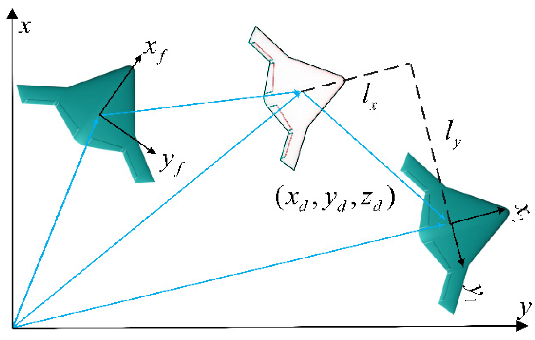
As shown in Figure 2, the geometry of the UAV formation is determined by the wingman’s position relative to the leading aircraft: longitudinal distance lx, lateral distance ly, and vertical distance lz. In tight-formation flight, the effect of the longitudinal distance lx on the induced forces and moments is much weaker than that of the lateral distance ly and vertical distance lz. Therefore, we do not discuss the effect of the longitudinal distance lx on the wake vortex here.
First, the induced velocity of the wake vortex was investigated. The induced velocity model used in this study is given in Equation (1). The vortex model [33] is based on a detailed analysis of LiDAR vortex tangential velocity observations, which draws conclusions that are valuable as a reference for the study of wake vortices in leading aircraft.
where Γ0 is the vortex strength of the wake vortex, b is the wing span, rc is the radius of the vortex nucleus (generally rc = 5.82%b) [34], and r is the vertical distance from the point of induced velocity to the vortex line.
The vortex strength is calculated using Equation (2):
where is the lift coefficient of the leader, b is the wing span and S is the wing area.
Suppose one point located on the wing of the following aircraft is at distance s from the right wingtip. At this point, the induced upwash velocity produced by the left tail vortex of the leading aircraft is , where , .
Similarly, the induced upwash velocity produced by the right tail vortex of the leading aircraft at this point is , where , .
The total velocity is
As such, the average induced upwash velocity on the wing of the wingman is calculated by integrating Equation (3), as shown in Equation (4):
As a result of the induced velocity, the lift force exerted on the wing of the wingman rotates, as shown in Figure 3.
V is the speed of the following aircraft, w is the induced upwash, and is the velocity of the wingman’s wing surface air. The initial lift and drag are denoted by L and D, respectively; the rotated lift and drag vectors are denoted by L’ and D’, respectively. Figure 3 shows that the change in the angle of attack of the aircraft is .
Because is small, Equation (5) can be approximated as . Figure 3 shows that the rotation of the lift force leads to a change in the value of the drag force to be
The increase in the drag coefficient is
The following aircraft’s increase in lift coefficient is
where is the slope of the following aircraft’s lift coefficient.
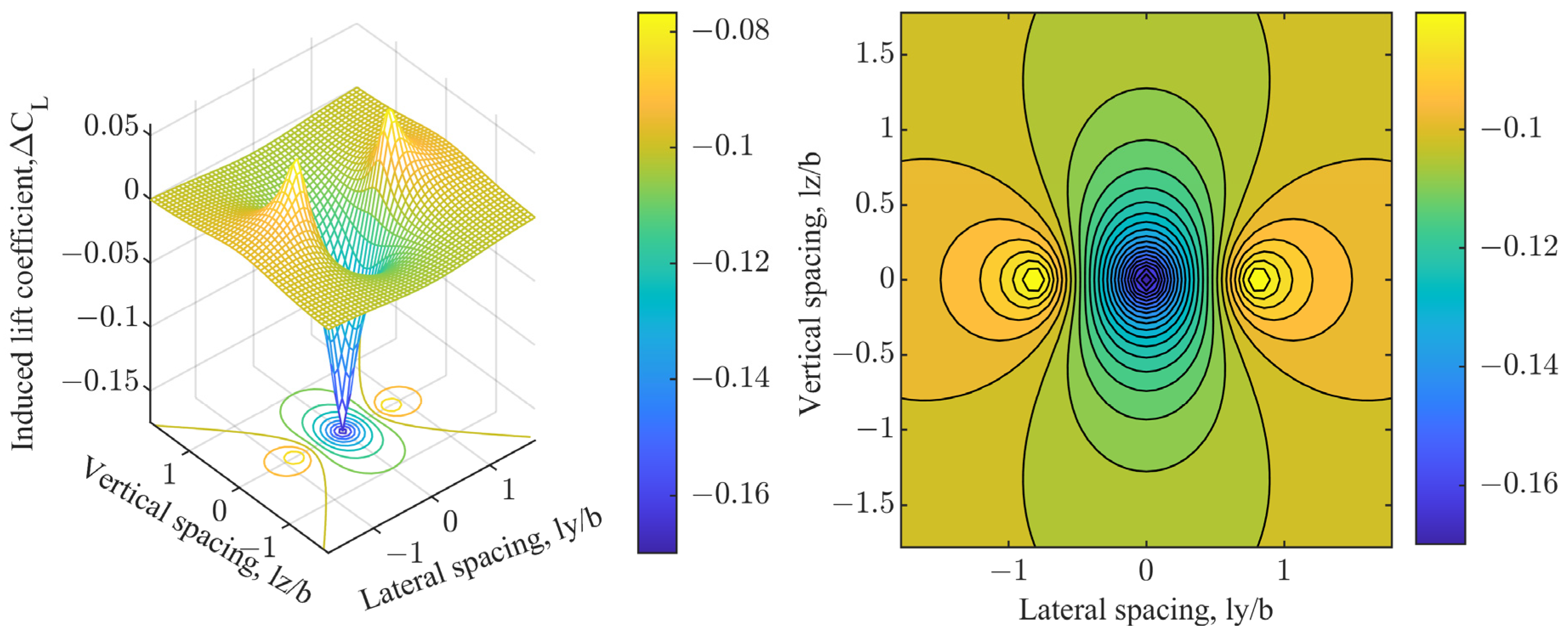
A schematic of the induced lift coefficients and the induced drag coefficients are shown in Figure 4 and Figure 5, respectively. The figures show two maximum values of the induced lift coefficient and two minimum values of the induced drag coefficient, which both occur close to the wingtip of the leading aircraft and are symmetrical between the left and right. Therefore, when studying the flight of aircraft in close formation, only the characteristics of one of the sides of the leading aircraft need to be studied. The induced lift coefficient reaches its maximum near and ; the induced drag coefficient reaches its minimum near and . To obtain both the maximum induced lift and maximum drag reduction, the lateral distance and vertical distance from the optimum point should be kept within 10% and 5% of the wingspan, respectively.
2.2. XFlow Software Calculation
Two UAVs flying in close formation were simulated using XFlow software, which allows the simulation of real atmospheric conditions through the setting of particle density. In the software, the wingman was placed to the right behind the leading aircraft, and the states of the leader and wingman at different positions were calculated by changing the relative positions of the wingman and leading aircraft. The main parameter settings of the XFlow software are shown in Table 1.
The lift and drag coefficients of the leader and wingman are shown in Figure 6 and Figure 7, respectively. When lx = 2b, lz = 0, by varying the relative positions of the wingman and leading aircraft, the maximum value of the lift coefficient occurs at ly = 0.875b (i.e., the wingtips of the leader and follower coincide by approximately 0.125b). Similarly, the minimum drag coefficient occurs at t ly = 0.875b. The results match those obtained with the developed mathematical model, with the aircraft obtaining the maximum tail vortex benefit when the wings of the two aircraft coincide at approximately 0.125b.
The following section describes the design of the robust controller that ensures that the follower maintains stable flight even in the presence of wake turbulence, thereby maximizing the advantages of flying in formation.
3. Design of Tight Formation Controller
The nonlinear kinematic equations for wingmen in close formation are shown in Equation (9).
where is the wingman’s position coordinates in the inertial coordinate system; are the airspeed, flight path, and heading angle, respectively; and is the induced wake velocity without considering external wind.
The formation flight system is described in an inertial coordinate system, as shown in Figure 8, where is the position of the leading aircraft in the inertial coordinate system; is the desired position for the wingman to follow, i.e., the optimal position for the follower in the formation flight system; and is the position of the follower in the inertial coordinate system. can be obtained from Equation (10).
where is the rotation matrix
The follower-to-desired-position error is projected on the aircraft’s body axis as
where is the desired heading angle of the following aircraft
After differentiating Equation (11), we obtain
3.1. Design of Extended State Observer
Equation (12) can be written as follows
where , , .
A nonlinear perturbation is used to estimate the disturbance of the wake vortex to which the follower is subjected, whereby the perturbation acting on the wingman is expanded into new state variable .
The system shown in Equation (13) is expanded into the new control system shown in Equation (14).
The uncertainty term is involved as a state variable, and the following expansion state observer was built for the system:
where , .
The error of the state observer is discussed next. From Equations (14) and (15), the error system can be obtained as
This error system ultimately reaches a steady state. When the positions of the two aircraft are established, . As such, we have
Furthermore, we can conclude that
Thus, as long as is sufficiently larger than , these steady-state errors are of the same order of magnitude as .
3.2. Design of Sliding Mode Controller
The designed extended state observer accurately estimated the perturbation experienced by the wingman, i.e., . By subtracting the estimated value of the disturbance from the control system, the controlled system is as follows:
Lemma 1
Lemma 1 is substantiated in [35] with a comprehensive proof.
In the subsequent analysis, the controller was designed to ensure that ex, ey, and ez in Equation (17) converge to zero. The detailed design procedure and stability proof of the controller for lateral error ey are presented below, with similar approaches applicable to the longitudinal and vertical errors.
The design sliding mode function .
where is the tracking error, .
We designed the control instruction as
where is a constant.
The stability was analyzed as follows:
Define the Lyapunov function as
Therefore,
From Lemma 1, we obtain
So,
Substituting the control law Equation (19) into Equation (22) produces
where .
The solution to inequality is
As such, . The asymptotic convergence of is proved.
After adding the disturbance compensation, the total control command is
Similarly, the control commands for the flight path angle and speed are respectively
4. Simulation and Experimental Verification
We built upon the results of previous studies, where the nonlinear model of the aircraft was previously developed, and each aircraft had a separate inner-loop flight control system. The tight-formation flight control system is shown in Figure 9. In this study, the mathematical model of the studied wake vortex was added as a disturbance to the aerodynamic model of the following aircraft. Then, the designed tight formation controller was verified via mathematical and semi-physical simulations. The leading aircraft was flying on a predetermined trajectory, and the initial position of the following aircraft was far from the leading aircraft. By comparing the designed tight-formation controller with the previous controller, the reliability and practicability of the sliding mode control method based on the expanded state observer were verified. The parameters of the aircraft are presented in Table 2.
4.1. Numerical Simulation
The numerical simulations were performed on the Simulink platform of MATLAB.
The initial states of the leading aircraft are , , , , , , , , , ; Whereas the initial states of the following aircraft are , , , , , , , , , , .
The relative positions of the aircraft at different moments of the formation flight are shown in Figure 10, and the aircraft trajectories are shown in Figure 11. From 0 to 250 s, the leading aircraft was flying straight and level, the following aircraft’s initial lateral distance from the leading aircraft was 1000 m, the wingman’s heading angle was negative (to reduce the lateral distance error), and, at 70 s, the lateral error was 0. At approximately 100 s, the longitudinal error reduced to zero. At this point, the following aircraft completed the approach to the leading aircraft from a far distance, and the two aircraft executed a tight formation. From 250 to 750 s, the aircraft turned, and the relative positions of the two aircraft slightly wavered but within acceptable ranges.
The comparison of the results of the sliding mode control effect, with and without ESO, are shown in Figure 12, Figure 13 and Figure 14. The results all indicate that the sliding mode control with ESO is more accurate, more strongly suppresses the influence of wake vortices, and shows more robustness. In comparing the model predictive control (MPC) algorithm with the proposed control algorithm in this paper, we see the robust controller designed in this paper provides advantages, including faster convergence and smaller static errors.
4.2. Experiments with Semi-physical Simulation Platform
The platform comprised the flight control system, radio communication equipment, UAV computer processing unit, and visual display unit, the structure of which is depicted in Figure 15. The flight control system generated precise control commands to govern the aircraft’s movements. The radio facilitated seamless communication between the leading and following UAVs. The computer was responsible for solving complex UAV data computations (airspeed, angle of attack, sideslip angle, rolling angular rates, pitching angular rates, yawing angular rates, roll angle, pitch angle, yaw angle, flight-path angle, and positional coordinates of the aircraft). The visual display unit provided real-time information on the formation’s position and status.
The simulation results of the tight formation were displayed with Tacview software (The version number of the software is 1.9.3), as shown in Figure 16. Tacview is a versatile tool for analyzing flight data. Within this experimental platform, Tacview receives data from the UAV computer and presents detailed information on the formation’s position and attitude.
The following aircraft consistently maintained the optimal relative position to the leading aircraft. According to the aforementioned experimental results, the proposed controller effectively mitigated interference and increased system robustness. The real-time nature of the system and the practicality of the control method were validated through experiments conducted on a distributed semi-physical simulation platform.
The semi-physical simulation verification demonstrated that the designed controller can successfully operate on this hardware platform and that the computational speed of the flight control board is sufficient for the control system. Communication delay is a critical factor for a formation system, as excessive communication delay can cause the instability in the tight formation flight system. The radios used in the semi-physical simulation experiments were capable of fulfilling the requirements of the control system.
5. Conclusions
This study investigated the scenario in which two aircraft fly in close formation. First, a mathematical model of the wake vortex was established. Second, Xflow software was employed to simulate the formation characteristics of the two UAVs. From the simulation results, we found that when the distance between the two UAVs is (lx = 2b, ly = 0.875b, lz = 0), the wingman experiences the maximum formation aerodynamic benefit. This finding aligns with the conclusion derived from studying wake vortex. Third, the disturbance of the wake vortex experienced by the wingman was then added to the wingman’s system, and a formation controller was developed that combines the extended state observer and sliding mode control methods. The controller considerably mitigated the effects on the following aircraft and enabled the following aircraft to maintain its optimal relative position to the leading aircraft. The designed formation control was validated, thus achieving the objectives through numerical and semi-physical simulations. In future studies, we will investigate the complex mechanisms of close-formation flight and the collision avoidance problems between the leading and following aircraft. Additionally, we will prepare for real close-formation flight experiments.
Author Contributions
Conceptualization, R.Z. and Q.Z.; Data curation, R.Z. and Y.L.; Methodology, R.Z. and S.H.; Software, R.Z. and Z.D.; Validation, R.Z. and J.S.; Writing—original draft, R.Z. All authors have read and agreed to the published version of the manuscript.
Funding
This research was funded by the National Natural Science Foundation of China, grant number 62373301 and 62173277; the Natural Science Foundation of Shaanxi Province, grant number 2023-JC-YB-526; the Aeronautical Science Foundation of China, grant number 20220058053002; and the Shaanxi Province Key Laboratory of Flight Control and Simulation Technology.
Data Availability Statement
The data presented in this study are available on request from the corresponding author.
Conflicts of Interest
The authors declare no conflicts of interest.
Nomenclature
| Γ0 | Vortex circulation |
| Lift coefficient of the leader | |
| The position coordinates of the leading aircraft | |
| The position coordinates of the following aircraft | |
| The bank, flight path, and heading angles | |
| The induced wake velocity | |
| S | Wing area |
| b | Wing span |
| Mean aerodynamic chord | |
| m | Gross mass |
| Ix | Roll moment of inertia |
| Iy | Pitch moment of inertia |
| Iz | Yaw moment of inertia |
| Ixz | Product moment of inertia |
References
- Li, W.-H.; Shi, J.-P.; Wu, Y.-Y.; Wang, Y.-P.; Lyu, Y.-X. A Multi-UCAV cooperative occupation method based on weapon engagement zones for beyond-visual-range air combat. Def. Technol. 2022, 18, 1006–1022. [Google Scholar] [CrossRef]
- Zhang, Q.; Liu, H.H.T. Aerodynamic model-based robust adaptive control for close formation flight. Aerosp. Sci. Technol. 2018, 79, 5–16. [Google Scholar] [CrossRef]
- Zhang, Q.; Liu, H.H. Robust Design of Close Formation Flight Control via Uncertainty and Disturbance Estimator. In Proceedings of the AIAA Guidance, Navigation, and Control Conference, San Diego, CA, USA, 4–8 January 2016. [Google Scholar]
- Frew, E.W.; Lawrence, D.A.; Morris, S. Coordinated standoff tracking of moving targets using Lyapunov guidance vector fields. J. Guid. Control Dyn. 2008, 31, 290–306. [Google Scholar] [CrossRef]
- Hansen, J.L.; Cobleigh, B.R. Induced Moment Effects of Formation Flight Using Two F/A-18 Aircraft. In Proceedings of the AIAA Atmospheric Flight Mechanics Conference and Exhibit, Monterey, CA, USA, 5–8 August 2002. [Google Scholar]
- Zheng, R.; Shi, J.; Qu, X. Modeling, Simulation and Control of Close Formation Flight. In Proceedings of the 2021 China Automation Congress (CAC), Beijing, China, 22–24 October 2021; pp. 3902–3907. [Google Scholar]
- Saban, D.; Whidborne, J.F.; Cooke, A.K. Simulation of wake vortex effects for UAVs in close formation flight. Aeronaut. J.-New Ser. 2009, 113, 727–738. [Google Scholar] [CrossRef]
- Lissaman, P.B.; Shollenberger, C.A. Formation flight of birds. Science 1970, 168, 1003–1005. [Google Scholar] [CrossRef] [PubMed]
- Cutts, C.J.; Speakman, J.R. Energy Savings in Formation Flight of Pink-Footed Geese. J. Exp. Biol. 1994, 189, 251–261. [Google Scholar] [CrossRef] [PubMed]
- Rayner, J. Estimating power curves of flying vertebrates. J. Exp. Biol. 1999, 202, 3449–3461. [Google Scholar] [CrossRef] [PubMed]
- Weimerskirch, H.; Martin, J.; Clerquin, Y.; Alexandre, P.; Jiraskova, S. Energy saving in flight formation. Nature 2001, 413, 697–698. [Google Scholar] [CrossRef] [PubMed]
- Cho, H.; Han, C. Effect of sideslip angle on the aerodynamic characteristics of a following aircraft in close formation flight. J. Mech. Sci. Technol. 2015, 29, 3691–3698. [Google Scholar] [CrossRef]
- Vachon, M.J.; Ray, R.J.; Walsh, K.R.; Ennix, K. F/A-18 Performance Benefits Measured during the Autonomous Formation Flight Project; Armstrong Flight Research Center: Edwards Air Force Base, CA, USA, 2013. [Google Scholar]
- Vicroy, D.; Vijgen, P.; Reimer, H.; Gallegos, J.; Spalart, P. Recent NASA wake-vortex flight tests, flow-physics database and wake-development analysis. In Proceedings of the AIAA and SAE, 1998 World Aviation Conference, Anaheim, CA, USA, 28–30 September 1998. [Google Scholar]
- Kent, T.E.; Richards, A.G. Analytic approach to optimal routing for commercial formation flight. J. Guid. Control Dyn. 2015, 38, 1872–1884. [Google Scholar] [CrossRef]
- Pahle, J.; Berger, D.; Venti, M.; Duggan, C.; Faber, J.; Cardinal, K. An initial flight investigation of formation flight for drag reduction on the C-17 aircraft. In Proceedings of the AIAA Atmospheric Flight Mechanics Conference, Minneapolis, MN, USA, 13–16 August 2012; p. 4802. [Google Scholar]
- Bieniawski, S.R.; Rosenzweig, S.; Blake, W.B. Summary of flight testing and results for the formation flight for aerodynamic benefit program. In Proceedings of the 52nd Aerospace Sciences Meeting, National Harbor, MD, USA, 13–17 January 2014; p. 1457. [Google Scholar]
- Hanson, C.E.; Pahle, J.; Reynolds, J.R.; Andrade, S.; Nelson, B. Experimental measurements of fuel savings during aircraft wake surfing. In Proceedings of the 2018 Atmospheric Flight Mechanics Conference, Atlanta, GA, USA, 25–29 June 2018; p. 3560. [Google Scholar]
- Okolo, W.; Dogan, A.; Blake, W. Effect of trail aircraft trim on optimum location in formation flight. J. Aircr. 2015, 52, 1201–1213. [Google Scholar] [CrossRef]
- Zhang, Q.; Pan, W.; Reppa, V. Model-reference reinforcement learning for collision-free tracking control of autonomous surface vehicles. IEEE Trans. Intell. Transp. Syst. 2021, 23, 8770–8781. [Google Scholar] [CrossRef]
- Blake, W.B.; Gingras, D.R. Comparison of Predicted and Measured Formation Flight Interference Effects. J. Aircr. 2004, 41, 201–207. [Google Scholar] [CrossRef]
- Ray, R.; Cobleigh, B.; Vachon, M.; St. John, C. Flight Test Techniques used to Evaluate Performance Benefits During Formation Flight. In Proceedings of the AIAA Atmospheric Flight Mechanics Conference and Exhibit, Monterey, CA, USA, 5–8 August 2002.
- Wilson, D.B.; Goktogan, A.H.; Sukkarieh, S. A Vision Based Relative Navigation Framework for Formation Flight. In Proceedings of the 2014 IEEE International Conference on Robotics & Automation (ICRA), Hong Kong, China, 31 May–7 June 2014. [Google Scholar]
- Zheng, R.; Lyu, Y. Nonlinear tight formation control of multiple UAVs based on model predictive control. Def. Technol. 2023, 25, 69–75. [Google Scholar] [CrossRef]
- Zhang, Q.; Liu, H.H.T. Robust Nonlinear Close Formation Control of Multiple Fixed-Wing Aircraft. J. Guid. Control Dyn. 2021, 44, 572–586. [Google Scholar] [CrossRef]
- Pachter, M.; D’Azzo, J.J.; Proud, A.W. Tight formation flight control. J. Guid. Control Dyn. 2001, 24, 246–254. [Google Scholar] [CrossRef]
- Binetti, P.; Ariyur, K.B.; Krstic, M.; Bernelli, F. Formation flight optimization using extremum seeking feedback. J. Guid. Control Dyn. 2003, 26, 132–142. [Google Scholar] [CrossRef]
- Chichka, D.F.; Speyer, J.L.; Fanti, C.; Park, C.G. Peak-seeking control for drag reduction in formation flight. J. Guid. Control Dyn. 2006, 29, 1221–1230. [Google Scholar] [CrossRef]
- Zhang, Q.; Liu, H.H.T. UDE-Based Robust Command Filtered Backstepping Control for Close Formation Flight. IEEE Trans. Ind. Electron. 2018, 65, 8818–8827. [Google Scholar] [CrossRef]
- Zhang, Q.; Liu, H.H. Robust cooperative close formation flight control of multiple unmanned aerial vehicles. In Proceedings of the Advances in Motion Sensing and Control for Robotic Applications: Selected Papers from the Symposium on Mechatronics, Robotics, and Control (SMRC’18)-CSME International Congress 2018, Toronto, ON, Canada, 27–30 May 2018; Springer: Cham, Switzerland, 2019; pp. 61–74. [Google Scholar]
- Ren, C.; Li, X.; Yang, X.; Ma, S. Extended state observer-based sliding mode control of an omnidirectional mobile robot with friction compensation. IEEE Trans. Ind. Electron. 2019, 66, 9480–9489. [Google Scholar] [CrossRef]
- Ding, S.; Hou, Q.; Wang, H. Disturbance-observer-based second-order sliding mode controller for speed control of PMSM drives. IEEE Trans. Energy Convers. 2022, 38, 100–110. [Google Scholar] [CrossRef]
- Proctor, F.; Hamilton, D.; Han, J. Wake vortex transport and decay in ground effect-Vortex linking with the ground. In Proceedings of the 38th Aerospace Sciences Meeting and Exhibit, Reno, NV, USA, 10–13 January 2000; p. 757. [Google Scholar]
- Proctor, F. Numerical simulation of wake vortices measured during the Idaho Falls and Memphis field programs. In Proceedings of the 14th Applied Aerodynamics Conference, New Orleans, LA, USA, 17–20 June 1996; p. 2496. [Google Scholar]
- Polycarpou, M.M.; Ioannou, P.A. A robust adaptive nonlinear control design. In Proceedings of the 1993 American Control Conference, San Francisco, CA, USA, 2–4 June 1993; pp. 1365–1369. [Google Scholar]
Figure 1.
Three views of the aircraft.

Figure 2.
Three views of the aircraft.

Figure 3.
Side view of wingman’s wing lift rotation.

Figure 4.
Variations in induced lift coefficient with lateral and vertical spacing.

Figure 5.
Variations in induced drag coefficient with lateral and vertical spacing.

Figure 6.
Lift coefficients for leader and follower (lx = 2b, lz = 0).

Figure 7.
Drag coefficients for leader and follower (lx = 2b, lz = 0).

Figure 8.
Schematic of the formation flight.

Figure 9.
Schematic of tight formation flight control system.

Figure 10.
Relative positions of aircraft at different times during formation flight.

Figure 11.
Formation trajectory.

Figure 12.
Longitudinal tracking error.

Figure 13.
Lateral tracking error.

Figure 14.
Vertical tracking error.

Figure 15.
Architecture diagram of distributed semi-physical simulation platform.

Figure 16.
Display of close formation flights in Tacview software.


Table 1.
Parameters of the XFlow software.
| Parameter | Value | Unit |
|---|---|---|
| Velocity | 27.8 | m/s |
| Mach number | 0.082 | |
| Reynolds number | 827,600 | |
| Particle resolution (Far field) | 1.28 | m |
| Particle resolution (Near field) | 0.0025 | m |
| Reference area | 0.11175 | m2 |
| Simulation time | 0.06 | s |
Table 2.
Parameters of the UAV.
| Parameter | Symbol | Value | Unit |
|---|---|---|---|
| Wing area | S | 1.546 | m2 |
| Wing span | b | 2.808 | m |
| Mean aerodynamic chord | 0.78 | m | |
| Gross mass | m | 15 | kg |
| Roll moment of inertia | Ix | 2.369 | Kg·m2 |
| Pitch moment of inertia | Iy | 1.211 | Kg·m2 |
| Yaw moment of inertia | Iz | 3.522 | Kg·m2 |
| Product moment of inertia | Ixz | 0.022 | Kg·m2 |
Disclaimer/Publisher’s Note: The statements, opinions and data contained in all publications are solely those of the individual author(s) and contributor(s) and not of MDPI and/or the editor(s). MDPI and/or the editor(s) disclaim responsibility for any injury to people or property resulting from any ideas, methods, instructions or products referred to in the content. |
© 2024 by the authors. Licensee MDPI, Basel, Switzerland. This article is an open access article distributed under the terms and conditions of the Creative Commons Attribution (CC BY) license (https://creativecommons.org/licenses/by/4.0/).
Share and Cite
MDPI and ACS Style
Zheng, R.; Zhu, Q.; Huang, S.; Du, Z.; Shi, J.; Lyu, Y. Extended State Observer-Based Sliding-Mode Control for Aircraft in Tight Formation Considering Wake Vortices and Uncertainty. Drones 2024, 8, 165. https://doi.org/10.3390/drones8040165
AMA Style
Zheng R, Zhu Q, Huang S, Du Z, Shi J, Lyu Y. Extended State Observer-Based Sliding-Mode Control for Aircraft in Tight Formation Considering Wake Vortices and Uncertainty. Drones. 2024; 8(4):165. https://doi.org/10.3390/drones8040165
Chicago/Turabian StyleZheng, Ruiping, Qi Zhu, Shan Huang, Zhihui Du, Jingping Shi, and Yongxi Lyu. 2024. "Extended State Observer-Based Sliding-Mode Control for Aircraft in Tight Formation Considering Wake Vortices and Uncertainty" Drones 8, no. 4: 165. https://doi.org/10.3390/drones8040165