Distributed Localization for UAV–UGV Cooperative Systems Using Information Consensus Filter

Abstract

In the evolving landscape of autonomous systems, the integration of unmanned aerial vehicles (UAVs) and unmanned ground vehicles (UGVs) has emerged as a promising solution for improving the localization accuracy and operational efficiency for diverse applications. This study introduces an Information Consensus Filter (ICF)-based decentralized control system for UAVs, incorporating the Control Barrier Function–Control Lyapunov Function (CBF–CLF) strategy aimed at enhancing operational safety and efficiency. At the core of our approach lies an ICF-based decentralized control algorithm that allows UAVs to autonomously adjust their flight controls in real time based on inter-UAV communication. This facilitates cohesive movement operation, significantly improving the system resilience and adaptability. Meanwhile, the UAV is equipped with a visual recognition system designed for tracking and locating the UGV. According to the experiments proposed in the paper, the precision of this visual recognition system correlates significantly with the operational distance. The proposed CBF–CLF strategy dynamically adjusts the control inputs to maintain safe distances between the UAV and UGV, thereby enhancing the accuracy of the visual system. The effectiveness and robustness of the proposed system are demonstrated through extensive simulations and experiments, highlighting its potential for widespread application in UAV operational domains.

1. Introduction

In recent years, Unmanned Aerial Vehicles (UAVs) and Unmanned Ground Vehicles (UGVs) have captured increasing attention and interest. These vehicles have shown significant potential in various domains, such as search and rescue, surveillance, and environmental monitoring [1]. UAVs and UGVs are typically equipped with a variety of sensors, cameras, and other devices, enabling them to perform tasks including conducting search and rescue operations at disaster sites, monitoring potential danger zones, and environmental surveillance [2]. Their unmanned nature allows them to execute hazardous tasks, thus avoiding risks to human lives [3].

When these UAVs and UGVs form a cooperative system, they complement each other’s capabilities, leveraging their respective strengths to accomplish more complex missions [4]. For instance, UAVs can provide high-altitude perspectives and rapid response capabilities [5], while UGVs can offer a stable platform and longer duration of sustained operations [6]. Their collaboration enhances the efficiency of the entire system, improving the effectiveness and accuracy of the work [7].

However, operating these vehicles in a coordinated manner proves to be a challenging task, especially in dynamic and uncertain environments [8]. Localizing UAVs becomes a specific challenge when they operate in tandem with other UAVs or UGVs, particularly in situations where Global Positioning System (GPS) signals are unavailable [9]. This urgent need for localization has led to the emergence of pioneering studies aimed at addressing this challenge [10]. Moreover, an algorithm is proposed to localize the UAVs using satellite images in [11]. The objective of these studies is to devise inventive solutions that empower UAVs to ascertain their position with precision, even in environments devoid of GPS signals.

Accurate localization information is essential for collaborative operations involving multiple unmanned vehicles. Hence, advancements in sensor technology have played an important role in enhancing the localization capabilities of UAVs and UGVs [12]. For instance, the integration of visual odometry, which relies on the analysis of camera images to estimate the motion of a vehicle, has emerged as a promising approach in environments where traditional GPS-based navigation is ineffective. Additionally, the use of Light Detection and Ranging (LiDAR) and radar technologies for mapping and navigation in complex terrains has gained traction [13]. These technologies enable UAVs and UGVs to create high-resolution maps of their surroundings, facilitating more precise positioning and maneuvering. Nevertheless, sensor technology may face limitations in precision, leading to less accurate data acquisition and consequently impacting the precision of localization information. Moreover, some sensors may exhibit sensitivity to environmental conditions such as changes in weather and variations in lighting, potentially compromising the sensor performance and, in turn, affecting the localization accuracy [14].

Simultaneously, machine learning algorithms, specifically within deep learning, have significantly advanced the localization capabilities of UAVs and UGVs. In [15], a vision-based algorithm is introduced to localize the targets using the UAV–UGV cooperative systems. Through the utilization of neural networks, these vehicles are now capable of processing extensive sensor data in real time, enabling them to make more precise and adaptable decisions [16]. Such capability proves critical in scenarios characterized by rapidly changing environmental conditions [17]. Conversely, deep learning algorithms often necessitate extensive datasets for training to achieve precise models [18]. Acquiring substantial training data in UAVs and UGVs might be constrained, particularly in intricate or perilous environments. Deep learning models might exhibit sensitivity to alterations in the environment, necessitating retraining or recalibration when the environmental conditions fluctuate, potentially impacting the accuracy of the localization information.

Furthermore, the integration of UAVs and UGVs into cooperative systems also offers prospects for leveraging swarm intelligence [19]. Through coordinated operations, these vehicles can exchange localization data and insights, enhancing the accuracy and efficiency of their endeavors. This swarm-based approach not only bolsters the capabilities of individual vehicles but also extends their operational scope and resilience in demanding environments [20]. In [21], a coalition formation game approach is proposed to localize the UAV swarm in a GNSS-denied environment.

Moreover, the establishment of standardized communication protocols and interoperable software frameworks is imperative for the smooth integration of UAVs and UGVs into a collaborative system [22]. These frameworks guarantee dependable and efficient data exchange and coordination among diverse vehicle types, thereby contributing their overall performance as a collective entity.

To cope with the aforementioned challenges, the expanding potential applications of UAVs and UGVs within cooperative systems signify a significant advancement in autonomous technology. Their versatility across various sectors, from agricultural monitoring [23] to urban planning [24], demonstrates their adaptability to diverse environments and tasks. Particularly notable is their ability to operate effectively in GPS-denied environments, overcoming the existing limitations and unlocking new opportunities for these technologies. This adaptability is crucial in addressing the challenges posed by inaccessible or compromised GPS signals, ensuring uninterrupted operations and broadening the application scope for UAVs and UGVs. Consequently, their capability to autonomously navigate and perform tasks in such conditions represents an essential step forward in the evolution of autonomous vehicle technology.

Recently, numerous solutions for UAV–UGV collaboration have emerged. UAVs and UGVs have garnered attention for their potential in high-risk missions, necessitating an effective cooperative control framework to optimize mission completion and resource utilization, particularly in applications like wildfire fighting [25]. However, their adaptability to dynamic environments may pose constraints, and relying on a central mobile mission controller for decisionmaking and planning could elevate the risk of system failure due to a single point of failure. In hazardous industrial settings, a decentralized scheme employs a drone to lead ground mobile robots transporting objects, with one robot navigating obstacles using drone-provided waypoints and a human operator while the others maintain distance and bearing through predictive vision-based tracking [26]. However, this scheme places high demands on the reliability and precision of both the drone and human operator, potentially leading to a lack of robustness. Failures or errors regarding either the drone or the operator could adversely affect the overall performance of the system. Reference [27] presents a cooperative UAV–UGV team for aerial tasks, proposing a control framework validated experimentally for efficient operation and reduced energy use. While UAVs and UGVs can assist each other, ensuring they do not cause damage or pose danger during task execution remains a challenge in real-world environments.

Distributed algorithms are computational procedures designed for systems consisting of multiple computing nodes [28]. These algorithms distribute tasks among the nodes, enabling them to collaborate and communicate in achieving a common objective. Each node in a distributed system possesses its own computational resources and local state [29]. Distributed algorithms play a critical role in the coordination and operation of UAVs and UGVs. In [30], a distributed solution mechanism is employed to determine the information-maximizing trajectories subject to the constraints of individual vehicle and sensor sub-systems. Additionally, ref. [31] demonstrates a considerable advantage of distributed UGVs over the static placement of control stations. These distributed algorithms facilitate communication and collaboration among the UAVs and UGV, allowing them to work together effectively to accomplish tasks.

The Information Consensus Filter (ICF) is a distributed algorithm used in multi-agent systems for estimating a common state [32]. It iteratively updates each agent’s estimate based on the local observations and received information from neighboring agents, using a consensus matrix to determine the weights of these updates. Through iterative consensus iterations, the ICF enables the agents to converge towards a consistent estimate of the common state, making it valuable for distributed estimation and control in dynamic environments. The ICF in UAV and UGV systems promotes information exchange and maintains state coherence across various Unmanned Aerial Vehicles and Unmanned Ground Vehicles. By fostering communication and collaboration among individual UAVs and UGVs, the ICF ensures a unified estimation of the shared states, thereby optimizing the task performance and resource utilization. Its implementation bolsters the system coordination and resilience, allowing for adept navigation in intricate environments and expanded utility across diverse applications. In [33], a distributed information filter algorithm is developed for each UGV to locally estimate the position and velocity of the quadrotor using its information and information from neighboring UGVs. Despite the pioneering advantages, the aforementioned research overlooks the integration of localization and control in unmanned vehicles.

1.1. Motivations

Improving the robustness and reliability of cooperative UAV–UGV systems is driven by the need to overcome challenges. This involves lessening the burdens on individual drones and human operators, ensuring adaptability to changing environments, and decreasing dependence on centralized control. The goal is to enhance the overall performance and safety of these systems in real-world scenarios. In response to the complexities of coordinating vehicle operations and guaranteeing precise localization data, we devised and executed a cost-effective vision-centered collaborative framework. While fully considering the superiority of distributed algorithms such as the ICF, our framework draws inspiration from the integration of UAVs and UGVs into cooperative systems and also incorporates the establishment of standardized communication protocols. It is engineered to dynamically adapt to changing environmental conditions, prioritize vehicle safety, and establish a reliable and efficient communication infrastructure. Additionally, it is engineered to accommodate multiple vehicles and facilitate seamless collaboration among them.

1.2. Contributions

We have developed and implemented a system that incorporates an advanced decentralized control algorithm and employs a Control Barrier Function–Control Lyapunov Function (CBF–CLF) strategy for UAVs, aimed at enhancing safety and efficiency. The efficacy of our system is validated through simulations of real-world scenarios.

In summary, the contributions are elaborated as follows:

• Distributed Algorithm Design: Our system integrates an advanced decentralized control algorithm, allowing UAVs to autonomously adapt control inputs in real time by leveraging data from the Information Consensus Filter (ICF). This decentralized strategy enables each UAV to function independently yet maintain cohesion within a larger fleet, bolstering system resilience and adaptability.
• Control Algorithm Design: At the core of our system is the Control Barrier Function–Control Lyapunov Function (CBF–CLF) strategy. This innovative control scheme emphasizes the safety of UAVs, which is essential for ensuring operational integrity. By enforcing safe separation distances between UAVs and obstacles, the CBF–CLF strategy minimizes collision risks. The continuous adjustment of control inputs, informed by real-time assessments of the vehicle’s state and surroundings, ensures effective implementation.
• Real-World Implementation: We evaluated the effectiveness and robustness of our system through extensive simulations in various real-world scenarios. This practical testing confirms the readiness of our system for real-world applications and sets the stage for its deployment in diverse UAV operational domains.

In comparison to the existing research methods, our system addresses several key limitations. Despite the high demands placed on the reliability and precision of both the drone and human operator, which could potentially lead to a lack of robustness, our system mitigates this risk through the incorporation of an advanced decentralized control algorithm. This algorithm enables UAVs to independently adjust the control inputs in real time via the Information Consensus Filter (ICF), reducing the dependency on precise human intervention and enhancing the overall system resilience. Additionally, while their adaptability to dynamic environments may pose constraints, our system’s decentralized approach allows for greater flexibility in responding to changing conditions. Furthermore, the reliance on a central mobile mission controller for decisionmaking and planning, which could elevate the risk of system failure due to a single point of failure, is minimized in our system by distributing the decisionmaking processes across the UAV fleet. Finally, while UAVs and UGVs can assist each other, ensuring that they do not cause damage or pose danger during task execution remains a challenge in real-world environments. However, our system addresses this challenge through the implementation of the Control Barrier Function–Control Lyapunov Function (CBF–CLF) strategy, which prioritizes UAV safety by enforcing safe separation distances from obstacles, thereby reducing collision risks. Through extensive simulation-based evaluations across various real-world scenarios, our system’s effectiveness and robustness were confirmed, affirming its readiness for diverse UAV operational domains.

The rest of this paper is organized as follows. Section 2.1 describes the preliminary knowledge of the distributed information for the cooperative systems and Control Lyapunov/Barrier Function. Afterwards, Section 2.2 provides the details regarding the proposed ICF-based Distributed UAV–UGV Cooperative System, including the system overview, dynamics, ICF for UAVs, and CBF–CLF for UAV–UGV Coopeative System. After that, extensive experimental results are presented in Section 3. Finally, the conclusion is provided in Section 4.

2. Materials and Methods

2.1. Preliminary Knowledge

2.1.1. Information-Weighted Consensus Filter

In the field of distributed systems, the ICF algorithm has emerged as a powerful algorithm for achieving consensus among multiple agents, even with limited communication and information exchange. It enables distributed entities to collaboratively estimate a common state or variable, utilizing local measurements and restricted information sharing.

Envision a distributed system consisting of N agents, indicated as $A_1,A_2,\dots ,A_N$. Every agent $A_i$ conducts its own local measurement and assesses the overarching state or variable. The ICF’s objective is to foster a consensus on this global state estimation through a process of iterative updates and reciprocal information sharing among the agents. The system’s linear dynamic system is characterized as follows:

$$\mathit{x}(t+1)=\varphi \mathit{x}\left(t\right)+\mathit{\gamma }\left(t\right),$$

(1)

where $\mathit{x}$ is the state vector, $\varphi$ is the state transfer matrix, $\mathit{\gamma }\in (0,Q)$ is the process noise, and $\mathit{Q}$ is the process covariance.

At time t, node $A_i$ possesses the following inputs: prior state estimation $\widehat{\mathit{x}}{i}^{-}\left(t\right)$, prior information matrix $\mathit{J}{i}^{-}\left(t\right)$, observation matrix ${\mathit{H}}_i$, consensus rate parameter $ϵ$, and total consensus iterations K. Upon acquiring the measurement value ${\mathit{z}}_i$ and the measurement covariance matrix ${\mathit{R}}_{\mathit{i}}^{-1}$, the initialization of the consistency information parameters will be conducted using the following equation:

$${\mathit{V}}_i^0\leftarrow \frac{1}{N}{\mathit{J}}_i^{-}\left(t\right)+{\mathit{H}}_i^T{\mathit{R}}_i^{-1}{\mathit{H}}_i,$$

(2)

$${\mathit{v}}_i^0\leftarrow \frac{1}{N}{\mathit{J}}_i^{-}\left(t\right){\widehat{\mathit{x}}}_i^{-}\left(t\right)+{\mathit{H}}_i^T{\mathit{R}}_i^{-1}{\mathit{z}}_i.$$

(3)

Here, ${\mathit{V}}_i^0$ and ${\mathit{v}}_i^0$ represent the initial information matrix and vector, respectively. Subsequently, ${\mathit{V}}_i^{k-1}$ and ${\mathit{v}}_i^{k-1}$ are updated using the average consistency algorithm over K iterations. During each iteration, node $A_{i^{\prime }}$ transmits ${\mathit{V}}_i^{k-1}$ and ${\mathit{v}}_i^{k-1}$ to all neighboring nodes $A_{i^{\prime }}$, while simultaneously receives ${\mathit{V}}_{i^{\prime }}^{k-1}$ and ${\mathit{v}}_{i^{\prime }}^{k-1}$ sent from all neighboring nodes. The information is updated according to the following equation:

$${\mathit{V}}_i^{\kappa }\leftarrow {\mathit{V}}_i^{\kappa -1}+ϵ\sum _{i^{\prime }\in {\mathcal{N}}_i}({\mathit{V}}_{i^{\prime }}^{\kappa -1}-{\mathit{V}}_i^{\kappa -1}),$$

(4)

$${\mathit{v}}_i^{\kappa }\leftarrow {\mathit{v}}_i^{\kappa -1}+ϵ\sum _{i^{\prime }\in {\mathcal{N}}_i}({\mathit{v}}_{i^{\prime }}^{\kappa -1}-{\mathit{v}}_i^{\kappa -1}).$$

(5)

Next, the posterior state estimate and information matrix for time t can be computed using the information vector and information matrix after iterative updating. The equations are as follows:

$${\widehat{\mathit{x}}}_i^{+}\left(t\right)\leftarrow {\left({\mathit{V}}_i^K\right)}^{-1}{\mathit{v}}_i^K,$$

(6)

$${\mathit{J}}_i^{+}\left(t\right)\leftarrow N{\mathit{V}}_i^K.$$

(7)

Finally, state information for time $t+1$ can be predicted using following equation:

$${\widehat{\mathit{x}}}_i^{-}(t+1)\leftarrow \mathit{\varphi }{\widehat{\mathit{x}}}_i^{+}\left(t\right),$$

(8)

$${\mathit{J}}_i^{-}(t+1)\leftarrow {(\mathit{\varphi }{\left({\mathit{J}}_i^{+}\left(t\right)\right)}^{-1}{\mathit{\varphi }}^T+\mathit{Q})}^{-1}.$$

(9)

The ICF refines each agent’s estimates by incorporating the weighted average of estimates from neighboring agents. Through continuous information exchange and iterative updates, the agents progressively converge to reach a consensus on the estimated global state or variable.

In the subsequent sections, we will delve into the practical applications of the ICF in distributed systems.

2.1.2. Control Lyapunov/Barrier Function

For a continuous-time affine control system $\dot{\mathit{x}}=F(t,\mathit{x},u)$, where $\mathit{x}\in {\mathbb{R}}^n$ represents the state vector and $u\in {\mathbb{R}}^m$ denotes the control input, if F is Lipschitz continuous with respect to $\mathit{x}$ and u, and time t is piecewise continuous while u is also piecewise continuous at time t, then, given the initial conditions, the trajectory exists and remains unique. Given a dynamical system where $f:{\mathbb{R}}^n⟶{\mathbb{R}}^n$, $g:{\mathbb{R}}^n⟶{\mathbb{R}}^{n\times m}$ and $\mathit{x}$ is Lipschitz continuous

$$\dot{\mathit{x}}=f\left(\mathit{x}\right)+g\left(\mathit{x}\right)u.$$

(10)

If there exists a constant C such that the continuous differential function $V\left(\mathit{x}\right)$ satisfies the following conditions, then $V\left(\mathit{x}\right)$ is considered a Control Lyapunov Function with respect to $\mathit{x}$:

• ${\Omega }_c$:= { $\mathit{x}\in {\mathbb{R}}^{n}V\left(\mathit{x}\right):\le C$ }
• $V\left(\mathit{x}\right)>0,\forall s\in {\mathbb{R}}^n\setminus \{{\mathit{x}}_e\},V\left({\mathit{x}}_{\mathit{e}}\right)=0$
• ${inf}_{u\in U}\dot{V}(\mathit{x},u)<0,\forall \mathit{x}\in {\Omega }_c,\setminus \left\{{\mathit{x}}_e\right\}$.

If $V\left(\mathit{x}\right):{\mathbb{R}}^n⟶\mathbb{R}$ is continuously differentiable, positive definite, and radially unbounded, then $V\left(\mathit{x}\right)$ can be proven to be an Exponentially Stabilizing Control Lyapunov Function (ESCLF) using the equation, where $\lambda$ represents the upper bound on the decay rate of the Lyapunov function:

$$\exists u\in U,\lambda >0,\dot{V}(\mathit{x},u)+\lambda V\left(\mathit{x}\right)\le 0.$$

(11)

When $\mathit{x}$ belongs to the following set and $\dot{h\left(\mathit{x}\right)}\ge 0$, then $h\left(\mathit{x}\right)$ is considered to satisfy the conditions of Control Barrier Function:

• $\mathcal{C}=\mathit{x}\in D\subset {\mathbb{R}}^n:h\left(\mathit{x}\right)\ge 0$
• $\partial \mathcal{C}=\mathit{x}\in D\subset {\mathbb{R}}^n:h\left(\mathit{x}\right)=0$
• $Int\left(\mathcal{C}\right)=\mathit{x}\in D\subset {\mathbb{R}}^n:h\left(\mathit{x}\right)>0$

In practical systems, a lower bound on the attenuation rate $\gamma$ is usually specified for the system if $B\left(\mathit{x}\right):{\mathbb{R}}^n⟶\mathbb{R}$ is continuously differentiable, and u making $B\left(\mathit{x}\right)$ satisfy Equation (12) will keep the system safe at all times.

$$\exists u\in U,\gamma >0,\dot{B}(\mathit{x},u)+\gamma B\left(\mathit{x}\right)\ge 0.$$

(12)

CLF ensures stability of the controller, whereas CBF guarantees that the system meets safety constraints. Integrating these two approaches allows for the formulation of a quadratic programming problem.

The CBF–CLF QP function is defined as

$$\begin{array}{cc}\hfill & u^{*}=arg\underset{u={[u,\delta ]}^T}{min}\frac{1}{2}{u}^T\mathit{H}u+{\mathit{F}}^{T}u\hfill \\ \hfill & s.t.\left\{\begin{array}{cc}\hfill & L_{f}V\left(\mathit{x}\right)+L_{g}V\left(\mathit{x}\right)u+\lambda V\left(\mathit{x}\right)\le \delta ,\hfill \\ \hfill & L_{f}B\left(\mathit{x}\right)+L_{g}B\left(\mathit{x}\right)u+\gamma B\left(\mathit{x}\right)\ge 0,\hfill \end{array}\right.\hfill \end{array}$$

(13)

where $V\left(\mathit{x}\right)$ is the CLF function, $B\left(\mathit{x}\right)$ is the CBF function, $\mathit{H}$ is a positive definite matrix, while $\mathit{F}\in {\mathbb{R}}^{n\times m}$, $\delta$ serves as a relaxation factor.

The CBF–CLF QP function offers a computationally efficient method to ensure both safety and stability of the controlled system. By resolving the quadratic program, an optimal control input can be derived to minimize the cost function while satisfying the safety and input constraints.

In the subsequent sections, we will delve into the theoretical foundations and practical applications of the CBF–CLF QP function in control systems.

As shown in  Figure 1, the system configuration comprises two UAVs assigned to track a UGV, with an “Armor” object mounted on the UGV for positioning purposes. This setup allows the UAV’s camera to utilize visual algorithms to calculate the UGV’s pose. Initial visual experiments indicate that maintaining a specific range between the UAVs and the UGV yields optimal performance. Leveraging this observation, the CBF–CLF equation is developed. Moreover, to improve the precision of the gathered data, the two UAVs exchange information and refine the collected data using the ICF algorithm.

2.1.3. Vision-Based Localization for UAVs

Image processing is carried out using OpenCV—4.8.1 https://opencv.org/ (accessed on 27 September 2023, developed by Intel, Santa Clara, CA, USA). The camera captures an image, which is then converted to grayscale. The contours of the light bars are detected, and an algorithm is utilized to precisely identify the four vertices of the light bars for localization purposes, along with extracting other pertinent information.

The visual feature, denoted as “Armor” and employed for identification in this experiment, is illustrated in Figure 2. It consists of two light bars mounted parallel on a rectangular plate, both of equal length and width. Upon capturing the contours, the OpenCV boundingRect function is utilized to determine the minimum bounding rectangle encompassing the light bars. In an image, aside from the target identification object, various noise may be present, which can be eliminated by applying filters based on the geometric characteristics of the contours.

Considering variations in the distance and angles between the UAVs and UGV during movement, the mentioned constraints can be suitably relaxed within a specific range. The contours acquired after filtering should precisely depict the target light bars. By mathematical sorting, the highest and lowest points on the contours of the two light bars are discerned, determining the four boundary points of the rectangle. These points are subsequently employed for pose calculation.

In this paper, the PNP algorithm is used to calculate the camera’s pose. To enhance the accuracy and stability of the PNP solution, we base our calculations on the following assumption, where $l_1$ is the Armor plane, $l_2$ is the groud, $l_3$ is the camera plane.

Assumption 1.

$\left|\overrightarrow{AB}\right|$ is known and $l_1\Vert l_2\Vert l_3$, while $\overrightarrow{AB}\stackrel{\left|\right|}{=}\overrightarrow{DC}$.

Assumption 2.

Each UAV can communicate with its neighbors, transferring the relative position of moving target.

PNP, commonly used in 3D reconstruction and camera pose estimation, follows a typical 3D–2D pose estimation process. It requires real coordinates of N spatial points in a known world coordinate system and their projections onto the image plane. At least three pairs of points are necessary for this process. In this scenario, the 3D points in the world coordinate system and the 2D points in the image coordinate system are known, while the camera pose remains unknown.

In this paper, we employ the Direct Linear Transform (DLT) method for pose calculation, specifically using the solvePNP function in OpenCV. Geometric structure of PNP is shown in Figure 3.

The 3D coordinates of the Armor on the UGV in the world coordinate system can be expressed as

$$\begin{array}{c}\mathit{c}={\left[\begin{array}{c}{x}_w,y_w,z_w,1\end{array}\right]}^T.\end{array}$$

(14)

The 2D projected point of Armor in the image coordinate system can be expressed as

$$\begin{array}{c}\mathit{h}={\left[\begin{array}{c}u,v,1\end{array}\right]}^T.\end{array}$$

(15)

The intrinsic matrix of the camera can be expressed as

$$\mathit{w}=\begin{array}{c}\left[\begin{array}{ccc}{f}_x& 0& c_x\\ 0& f_y& c_y\\ 0& 0& 1\end{array}\right]\end{array}.$$

(16)

Therefore, the relationship between 2D points in camera image and 3D points in real world can be expressed as

$$\begin{array}{c}\lambda \left[\begin{array}{c}u\\ v\\ 1\end{array}\right]=\left[\begin{array}{ccc}{f}_x& 0& c_x\\ 0& f_y& c_y\\ 0& 0& 1\end{array}\right]\left[\begin{array}{cc}\mathit{R}& \mathit{t}\end{array}\right]\left[\begin{array}{c}{x}_w\\ y_w\\ z_w\\ 1\end{array}\right]\end{array},$$

(17)

where $\mathit{R}$ and $\mathit{t}$ represent the rotation matrix and translation vector, respectively, describing the Armor pose to be determined. Substituting the four sets of solutions will yield the final pose solution.

2.2. Methodology

2.2.1. Icf-Based Distributed UAV–UGV Cooperative System

UAV–UGV cooperative systems often operate in dynamic and unpredictable environments. Adapting localization algorithms to maintain accuracy in real time poses a considerable challenge. Techniques for restricting UAV within the working range for optimal camera performance while ensuring computational efficiency are needed. Additionally, as the number of UAVs and UGVs in the cooperative system increases, the complexity of distributed localization grows exponentially. Algorithms capable of handling large-scale deployments while maintaining accuracy and robustness are essential. Meanwhile, ensuring the resilience of the localization system to sensor failures and communication disruptions is critical to information processing.

Based on the previous discussion, we have innovatively proposed the ICF-based Distributed UAV–UGV Cooperative System, providing a solution to the above-mentioned problems. The implementation of CBF–CLF equations serves to regulate the distance between the UAVs and UGV, ensuring data accuracy and integrity. By limiting the distance, each sensor operates within its optimal performance range. Moreover, to achieve complete coverage within the UAV’s FOV, we increase the number of UAVs and strategically position them. Additionally, we employ the ICF algorithm to facilitate data exchange among UAVs, enabling data fusion to address the issue of naive nodes and enhance state estimation. In essence, the two algorithms in the proposed system run independently, providing a practical dual guarantee of data accuracy from different aspects, optimizing individual camera data computations while ensuring data integrity and robust state estimation. The schematic diagram of ICF-based Distributed UAV–UGV Cooperative System is shown in Figure 4.

2.2.2. Dynamics

We commence by formulating the system dynamics. Our model assumes linear trajectories for both the UAV and the UGV, with both vehicles consistently maintaining aligned directions.

The velocity of UGV ${\mathit{v}}_l\left(t\right)$ can be calculated using Equation (18), where $\mathit{D}\left(t\right)$ is the relative displacement of the UGV, ${\mathit{v}}_f$ is the velocity of UAV, and $\Delta T$ is the time interval between t and $t+1$.

$${\mathit{v}}_l\left(t\right)={\mathit{v}}_f\left(t\right)+\frac{\mathit{D}\left(t\right)-\mathit{D}(t-1)}{△T}.$$

(18)

During the simulation, ${\mathit{v}}_f\left(t\right)$ will be updated at each time t using ${\mathit{\alpha }}_l\left(t\right)$, the acceleration of UAV. It can be updated by

$${\mathit{v}}_f\left(t\right)={\mathit{v}}_f(t+1)+{\mathit{\alpha }}_f\left(t\right)△T.$$

(19)

The acceleration of the UAV is represented as

$${\mathit{\alpha }}_f\left(t\right)=\frac{u\left(t\right)-F_r\left({\mathit{v}}_f\left(t\right)\right)}{M}.$$

(20)

The dynamics of the system can be expressed as

$$\dot{\mathit{x}}\left(t\right)=\underset{f\left({\mathit{x}}_i\right)\left(t\right)}{\underbrace{\left[\begin{array}{c}-F_r\left({\mathit{v}}_f\left(t\right)\right)/M\\ {\mathit{\alpha }}_f\left(t\right)\\ {\mathit{v}}_l\left(t\right)-{\mathit{v}}_f\left(t\right)\end{array}\right]}}+\underset{g\left({\mathit{x}}_i\right)\left(t\right)}{\underbrace{\left[\begin{array}{c}1/M\\ 0\\ 0\end{array}\right]}}u\left(t\right).$$

(21)

Here, $x=(x_1,x_2,x_3)=({\mathit{v}}_f\left(t\right),{\mathit{v}}_l\left(t\right),\mathit{D}\left(t\right))$, M is the mass of the UAV, and $u\left(t\right)$ is the control input of UAV. In this equation, ${\mathit{v}}_f\left(t\right)$ can be regulated by feedback through $u\left(t\right)$. The aerodynamic drag values with constants $f_0$, $f_1$, and $f_2$ determined empirically are expressed as

$$F_r\left({\mathit{v}}_f\left(t\right)\right)=f_0+f_1{\mathit{v}}_f\left(t\right)+f_2{\mathit{v}}_f^2\left(t\right).$$

(22)

2.2.3. ICF for UAVs

The field of view (FOV) of a camera is typically limited. To ensure comprehensive coverage, it is common practice to deploy two or more UAVs equipped with cameras for tracking and measurement purposes. This arrangement guarantees that the trajectory of the UGV can be fully observed, and the fusion of measurement data from multiple UAVs significantly enhances the accuracy of the measurements.

We consider a continuous linear motion model with constant velocity:

$$\mathit{x}(t+1)=\mathit{M}\mathit{x}\left(t\right)+\mathit{\gamma }\left(t\right),$$

(23)

where $\mathit{M}$ is the state transition matrix, while $\mathit{\gamma }\left(t\right)\in N(0,\mathit{Q})$ is Gaussian process noise with positive definite covariance matrix $\mathit{Q}$.

During each time step t during the operation of the ICF, it requires K iterations to achieve consensus with neighboring UAVs regarding the current estimate of the UGV trajectory and the associated information matrix. This process is designed to maintain alignment with the neighboring estimates and pertinent information matrices related to the current UGV trajectory. Through multiple iterations, the ICF endeavors to synchronize and update information, thereby enhancing the overall consensus.

Simultaneously, it is crucial to ensure that the UGV remains continuously within the FOV of the UAVs. Importantly, it suffices for the UGV to be within the FOV of any UAV. Through the exchange of information with neighboring UAVs, the algorithm can partially extend the observation range, thereby maintaining data integrity. This characteristic represents a significant advantage of the algorithm. The average consensus algorithm is articulated as follows:

$${\mathit{x}}_i^{\kappa }\leftarrow {\mathit{x}}_i^{\kappa -1}+ϵ\sum _{j\in {\mathcal{N}}_i}({\mathit{x}}_j^{\kappa -1}-{\mathit{x}}_i^{\kappa -1}).$$

(24)

Prediction for the next time step t can be expressed as

$${\widehat{\mathit{x}}}_i^{-}(t+1)\leftarrow \mathit{M}{\widehat{\mathit{x}}}_i^{+}\left(t\right),$$

(25)

$${\mathit{G}}_i^{-}(t+1)\leftarrow {(\mathit{M}{\left({\mathit{G}}_i^{+}\left(t\right)\right)}^{-1}{\mathit{M}}^T+\mathit{Q})}^{-1}.$$

(26)

Therefore, we obtain the ICF-based UAV–UGV cooperative system in Algorithm 1.

Algorithm 1: ICF at UAV i relative to UGV r at time step k

2.2.4. CBF–CLF for UAV–UGV Coopeative System

Based on the system’s dynamics model, we propose a soft constraint for the system, aiming to enable the UAV to achieve a desired speed.

$$V\left(\mathit{x}\right)={({\mathit{v}}_f-{\mathit{v}}_d)}^2.$$

(27)

Here, $V\left(\mathit{x}\right)$ is a continuously differentiable function, and, for any $c>0$, if the following inequality (28) holds, then $V\left(\mathit{x}\right)$ is a qualified CLF.

$$\underset{\mathit{u}\in \mathbb{R}}{inf}\left[{\mathcal{L}}_{f}V\left(\mathit{x}\right)+{\mathcal{L}}_{g}V\left(\mathit{x}\right)u+cV\left(\mathit{x}\right)\right]\le 0.$$

(28)

Next, we detail the hard constraints of this system. As previously mentioned, we aim for the distance between the UAVs and the UGV to remain within a specified range to ensure the high accuracy of data measured by the vision algorithm. We define these constraints as follows:

$$\begin{array}{c}\hfill \mathit{D}\ge {\tau }_1{\mathit{v}}_f,\\ \hfill \mathit{D}\le {\tau }_2{\mathit{v}}_f.\end{array}$$

(29)

Here, we propose two hard constraints: ${\tau }_1$ is the time when the UAV catches up with the UGV and the the distance exceeds $D_{max}$, and ${\tau }_2$ is the time when the UAV moves away from the UGV and distance narrows to within $D_{min}$. We consider the function $h_1\left(\mathit{x}\right)=\mathit{D}-{\mathit{v}}_f{\tau }_1$ and $h_2\left(\mathit{x}\right)={\mathit{v}}_f{\tau }_2-\mathit{D}$. Therefore, a candidate CBF can be expressed as

$$\begin{array}{cc}\hfill & B\left(\mathit{x}\right)=-log\left(\frac{h_1\left(\mathit{x}\right)}{1+h_1\left(\mathit{x}\right)}\right),\hfill \\ \hfill & C\left(\mathit{x}\right)=-log\left(\frac{h_2\left(\mathit{x}\right)}{1+h_2\left(\mathit{x}\right)}\right).\hfill \end{array}$$

(30)

We set $\gamma =1$ in the following equation, thus verifying that $B\left(\mathit{x}\right)$ and $C\left(\mathit{x}\right)$ are qualified CBFs.

$$\begin{array}{cc}\hfill & \underset{u\in \mathbb{R}}{inf}\left[{\mathcal{L}}_{f}B\left(\mathit{x}\right)+{\mathcal{L}}_{g}B\left(\mathit{x}\right)u-\frac{\gamma }{B\left(\mathit{x}\right)}\right]\le 0,\hfill \\ \hfill & \underset{u\in \mathbb{R}}{inf}\left[{\mathcal{L}}_{f}C\left(\mathit{x}\right)+{\mathcal{L}}_{g}C\left(\mathit{x}\right)u-\frac{\gamma }{C\left(\mathit{x}\right)}\right]\le 0.\hfill \end{array}$$

(31)

From this, we build the CLF–CBF QP problem based on the constraints established above.

$$\begin{array}{cc}\hfill & u^{*}=arg\underset{u={[u,\delta ]}^T}{min}\frac{1}{2}{u}^T{\mathit{H}}_{ag}u+{\mathit{F}}_{ag}^{T}u\hfill \\ \hfill & s.t.\left\{\begin{array}{cc}\hfill & {\mathit{A}}_{clf}u\le {\mathit{b}}_{clf},\hfill \\ \hfill & {\mathit{A}}_{cbf}u\le {\mathit{b}}_{cbf},\hfill \end{array}\right.\hfill \end{array}$$

(32)

where

$$\begin{array}{cc}\hfill & {\mathit{A}}_{clf}=\left[\begin{array}{cc}{\mathcal{L}}_{g}V\left(\mathit{x}\right)& -1\end{array}\right],\hfill \\ \hfill & {\mathit{A}}_{cbf}=\left[\begin{array}{cc}{\mathcal{L}}_{g}B\left(\mathit{x}\right)& 0\\ {\mathcal{L}}_{g}C\left(\mathit{x}\right)& 0\end{array}\right],\hfill \end{array}$$

(33)

$$\begin{array}{cc}\hfill & {\mathit{b}}_{\mathrm{clf}}=\left[\begin{array}{c}-L_{f}V\left(\mathit{x}\right)-cV\left(\mathit{x}\right)\end{array}\right],\hfill \\ \hfill & {\mathit{b}}_{\mathrm{cbf}}=\left[\begin{array}{c}-{\mathcal{L}}_{f}B\left(\mathit{x}\right)+\gamma \frac{1}{B\left(\mathit{x}\right)}\\ -{\mathcal{L}}_{f}C\left(\mathit{x}\right)+\gamma \frac{1}{C\left(\mathit{x}\right)}\end{array}\right],\hfill \end{array}$$

(34)

$$\begin{array}{c}\hfill \left\{\begin{array}{cc}\hfill & {\mathcal{L}}_{g}V\left(\mathit{x}\right)=\frac{2({\mathit{v}}_f-{\mathit{v}}_d)}{M},\hfill \\ \hfill & {\mathcal{L}}_{f}V\left(\mathit{x}\right)=\frac{2F_r({\mathit{v}}_f-{\mathit{v}}_d)}{M},\hfill \end{array}\right.\end{array}$$

(35)

$$\begin{array}{c}\hfill \left\{\begin{array}{cc}\hfill & {\mathcal{L}}_{g}B\left(\mathit{x}\right)=\frac{{\tau }_1}{M(1+h_1\left(\mathit{x}\right))h_1\left(\mathit{x}\right)},\hfill \\ \hfill & {\mathcal{L}}_{f}B\left(\mathit{x}\right)=\frac{-{\tau }_1{F}_r/M+{\mathit{v}}_l-{\mathit{v}}_f}{(1+h_1\left(\mathit{x}\right))h_1\left(\mathit{x}\right)},\hfill \end{array}\right.\end{array}$$

(36)

$$\begin{array}{c}\hfill \left\{\begin{array}{cc}\hfill & {\mathcal{L}}_{g}C\left(\mathit{x}\right)=\frac{-{\tau }_2}{M(1+h_2\left(\mathit{x}\right))h_2\left(\mathit{x}\right)},\hfill \\ \hfill & {\mathcal{L}}_{f}C\left(\mathit{x}\right)=\frac{{\tau }_2{F}_r/M+{\mathit{v}}_f-{\mathit{v}}_l}{(1+h_2\left(\mathit{x}\right))h_2\left(\mathit{x}\right)}.\hfill \end{array}\right.\end{array}$$

(37)

In Equation (32), $\delta$ represents the relaxation factor. Setting $\delta$ to zero enforces precise exponential convergence at the rate c. Under these conditions, the constraints imposed by the CLF become more stringent, complicating the acquisition of suitable solutions for the QP equation. Meanwhile, the CLF converts the stability issue of the system into an optimization problem, aiming to minimize or satisfy specific performance metrics, articulated through a cost function. The construction of the CLF begins with partially linearizing the system using the feedback $u=F_r+M\mathsf{\mu }$. Consequently, the cost function for this control mechanism is expressed as follows:

$$\mathsf{\mu }{\mathsf{\mu }}^T={|(F_r-u)/M|}^2=\frac{1}{M^2}\left(F_r^2+u^2-2u{F}_r\right).$$

(38)

This can then be converted into Equation (39), where $p_{sc}$ is the weight for the relaxation $\delta$.

$${\mathit{H}}_{ag}=2\left[\begin{array}{cc}\frac{1}{M^2}& 0\\ 0& p_{sc}\end{array}\right],{\mathit{F}}_{ag}=-2\left[\begin{array}{c}{F}_r/M^2\\ 0\end{array}\right].$$

(39)

Therefore, we obtain the CBF–CLF Tracking system in Algoritm 2.

Algorithm 2: CBF–CLF Tracking Algorithm.

3. Results

3.1. Vision-Based Localization

In the practical scenario where a UAV tracks a UGV, the UAV often needs to acquire the pose of the UGV for self-adjustment and decisionmaking. Computer vision algorithms are frequently employed to recognize the object’s pose. However, due to the limitations in the sensor precision and the inherent design of these algorithms, the computed results often exhibit errors. This issue becomes particularly pronounced in distance measurements using the Perspective-n-Point (PnP) algorithm, where increased distance can cause objects to appear blurry or smaller in the image. Consequently, this leads to the visual features used for localization becoming less distinct or sparse, challenging the algorithm’s ability to accurately match these feature points and affecting the precision of the pose estimation.

Given the aforementioned considerations, it is imperative to investigate the impact of distance variation on visual computation. With the knowledge of the camera’s performance across different distances, it becomes possible to regulate the accuracy of the data acquisition by adjusting the observation distance, thus optimizing the system performance. The parameters used for experiment are shown in

Table 1. Parameters for experiment.

Parameters Description	Value
Camera Model	MV-SUA133GC-T 1
Calibration error	0.24 pixel
The height of Armor	125 mm
The width of Armor	150 mm

¹ MindVision USB 3.0 Industrial Camera, Shenzhen, China.

.

The camera was positioned at various distances and angles relative to the Armor, and the previously mentioned visual algorithm was employed to identify the light bars on the Armor and calculate their poses and angles. The distance between the camera and the Armor was computed, and the measurement error was then compared with the actual distance. The positions of the UAVs in the experiment are predetermined based on the distribution of the experimental variables, and each position is carefully measured and set. In this way, the error of the algorithm can be accurately calculated. The experimental setup is shown in Figure 5.

The experiment involved two variables: distance and angle. The distance varied from 3 m to 5 m, in increments of ten centimeters, resulting in 11 groups. The angle started with the camera facing the Armor at 0 degrees and ranged up to 40 degrees to the left, in increments of ten degrees, creating five groups. Considering the symmetry in the recognition of the left and right deviations, focusing solely on the left deviations was deemed sufficient for meeting the research objective. Consequently, this experiment comprised a total of 110 datasets.

Considering that an excessively large yaw angle could result in the loss of one side of the light bars, thereby making it impossible to form the visual features necessary for the Armor recognition, the experiment avoided overly large angles. Consequently, 40 degrees was selected as the maximum angle for this experiment.

As depicted in Figure 6, the error margin of the measurement data tends to widen as the distance increases. Within the range of 300 to 410 cm, the measurement error mostly fluctuates within 5 cm. Beginning at 420 cm, the measurement error starts to escalate, exhibiting significant deviations from previous values, with fluctuations between 10 and 15 cm. Consequently, we identify 410 cm as the threshold for accurate measurement. Beyond this distance, the camera pose estimation regarding the UAVs is deemed inaccurate, whereas, within this range, the estimation is considered to be reasonably accurate.

Meanwhile, the results in Figure 6 indicate that the deviations in angles have a relatively minor impact on the accuracy. The change in the yaw angle of the UAV relative to the UGV from 0 to 40 degrees has a negligible effect on the measurement data, which is theoretically justifiable. The algorithm functions by extracting the features from the upper and lower vertices of two light bars and then obtaining the rectangle corners through sorting. Consequently, the accuracy of the calculation is not dependent on the thickness of the light bars. Although an increase in the yaw angle may cause the captured light bars to appear thinner, it does not hinder the calculation process. However, excessively large yaw angles may lead to one side of the light bar becoming invisible, thereby creating an unsolvable scenario. Consequently, it is imperative to maintain the yaw angle below a critical threshold to ensure continuous observation and data integrity.

3.2. ICF

The tracking system described in this paper closely resembles a linear system. Regarding the algorithm performance, we posit that the ICF is somewhat less effective than the Centralized Kalman Filter (CKF). In the CKF, the sensor nodes collect a substantial amount of target information, facilitating the high-precision data processing of the accumulated information.

However, a significant characteristic of the CKF is its high-dimensional state space, which leads to a marked increase in computational complexity. This makes it challenging to fulfill the real-time requirements of navigation systems. Moreover, the fault tolerance of the CKF is relatively low. Should any node within the system fail, its impact spreads through the filter, affecting the other states and making the navigation information output of the combined system unreliable. Therefore, in practical applications, the ICF is preferred for mobile systems due to these considerations.

Based on the analysis above, if the average error curve of the ICF closely approximates that of the CKF, it is considered that the ICF has achieved a satisfactory performance. In this section, we evaluate the performance of the proposed ICF simulation in MATLAB 2023a and compare it with that of the CKF. The simulation of the tracking trajectory computed by the ICF algorithm is shown in Figure 7.

Initially, we investigate the influence of the number of cameras on the experimental results. Given the hardware limitations, the FOV of the cameras remains constant. To ensure comprehensive UGV observations, increasing the number of cameras and strategically placing them becomes imperative for accurate UGV tracking. It is essential that the UAV trajectory falls within the FOV of at least one camera; otherwise, it is considered unobservable and disregarded.

In this paper, we introduce two experimental variables: Process Covariance $\mathit{Q}$ and Number of Consensus Iterations K. The UAVs are symmetrically distributed on both sides of the UGV. The input variables encompass the random refreshing of the UGV’s position and an initial distance of 2 m between each UAV and the UGV. The velocity of the UGV is set to 1.5 m/s, with both the UAV’s tracking speed and the UGV’s leading speed undergoing slight random variations. Consequently, the inputs for the simulation can be denoted as $\mathit{x}=(x_i,y_i,v_x,v_y)$. The observation matrix ${\mathit{H}}_i$ and state transition matrix $\mathit{M}$ are defined as follows:

$${\mathit{H}}_i=\left[\begin{array}{cccc}1& 0& 0& 0\\ 0& 1& 0& 0\end{array}\right],\mathit{M}=\left[\begin{array}{cccc}1& 0& 1& 0\\ 0& 1& 0& 1\\ 0& 0& 1& 0\\ 0& 0& 0& 1\end{array}\right].$$

(40)

3.2.1. Process Covariance Q

The elements on the diagonal of the noise matrix represent the variance of measurement errors in the system’s corresponding state variables. The magnitude of these diagonal elements significantly influences the filter’s estimation accuracy of the system state. Larger diagonal elements usually indicate higher measurement noise in the corresponding state variables, rendering the system more sensitive to the impact of measurement noise. In this experiment, we have configured four sets of variables:

$$\begin{array}{cc}\hfill & {\mathit{Q}}_1=\mathrm{Diag}(0.01,0.01,1,1),\hfill \\ \hfill & {\mathit{Q}}_2=\mathrm{Diag}(0.1,0.1,1,1),\hfill \\ \hfill & {\mathit{Q}}_3=\mathrm{Diag}(1,1,1,1),\hfill \\ \hfill & {\mathit{Q}}_4=\mathrm{Diag}(10,10,1,1).\hfill \end{array}$$

(41)

In Figure 8, the CKF error curve shows that the error values across all the datasets are predominantly within ten, maintaining a consistently low level. For the ICF error curve, the first dataset displays the lowest error values, with the errors generally staying within 10 and peaking at 12 at most. Initially, the ICF error curve closely mirrors the CKF curve, indicating the efficient performance of the ICF. However, as the noise values on the diagonal escalate, there is a corresponding increase in the error values, leading to a divergence between the ICF and CKF curves. In the fourth dataset, the ICF’s error values notably exceed 20, occasionally nearing 30, and the curve predominantly deviates from the CKF curve.

3.2.2. Consensus Iterations K

The parameter “total number of consensus iterations K” dictates the number of consensus iterations the algorithm undertakes throughout the process, significantly impacting the convergence and performance of the algorithm. The purpose of these consensus iterations is to ensure uniformity among the various nodes in a distributed system, allowing them to collaboratively estimate or deduce the system’s state. As illustrated in Figure 9, the error curve of the ICF initially shows a significant deviation from the CKF error curve. However, as the number of iterations increases, specifically after $K=4$, the error curve of the ICF effectively converges and becomes comparable to the CKF curve. Beyond this point, further increasing the number of iterations does not result in a marked improvement in the ICF’s performance.

A higher value of K denotes more iterations, which aids in bolstering the algorithm’s stability in achieving consensus, but this can lead to prolonged computation times, consequently affecting the algorithm’s convergence speed. Augmenting the number of consensus iterations could impose additional computational demands; hence, choosing an optimal K value necessitates a balance between algorithm performance and computational efficiency. Given the dynamic nature of system states, the selection of K should also consider these dynamics. Larger K values are preferable in scenarios where the system states evolve gradually.

3.3. CBF–CLF

The findings from the preceding visual experiments suggest that maintaining a reasonable distance between UAVs and UGV is crucial to ensure the integrity and clarity of the Armor imaging. This experiment was simulated in MATLAB 2023a, and the parameters in this experiment are shown in

Table 2. Parameters for experiment.

Parameters Description	Value	Parameters Description	Value
M	10 $\mathrm{kg}$	$v_f^0$ (case 1)	1.0 $\mathrm{m}/\mathrm{s}$
$f_0$	0.1 $\mathrm{N}$	$v_l^0$ (case 1)	1.5 $\mathrm{m}/\mathrm{s}$
${\mathit{f}}_{\mathbf{1}}$	5 $\mathrm{Ns}/\mathrm{m}$	${\mathit{v}}_{\mathit{f}}^{\mathbf{0}}$ (case 2)	0.9 $\mathrm{m}/\mathrm{s}$
${\mathit{f}}_{\mathbf{2}}$	0.25 ${\mathrm{Ns}}^2/\mathrm{m}$	${\mathit{v}}_{\mathit{l}}^{\mathbf{0}}$ (case 2)	0.5 $\mathrm{m}/\mathrm{s}$
${\mathit{\tau }}_{\mathbf{1}}$	1 s	${\mathit{p}}_{\mathit{sc}}$	10
${\mathit{\tau }}_{\mathbf{2}}$	3 s	$\mathit{c}$	4
$\Delta \mathit{t}$	1 s	${\mathit{D}}_{\mathbf{0}}$	10
${\mathit{v}}_{\mathit{d}}$	$v_l$ + 0.1 $\mathrm{m}/\mathrm{s}$	$\mathit{g}$	9.81 $\mathrm{m}/\mathrm{s}$

. The initial velocities of the UAV and UGV are selected under the consideration of platform capabilities, safety, and efficiency.

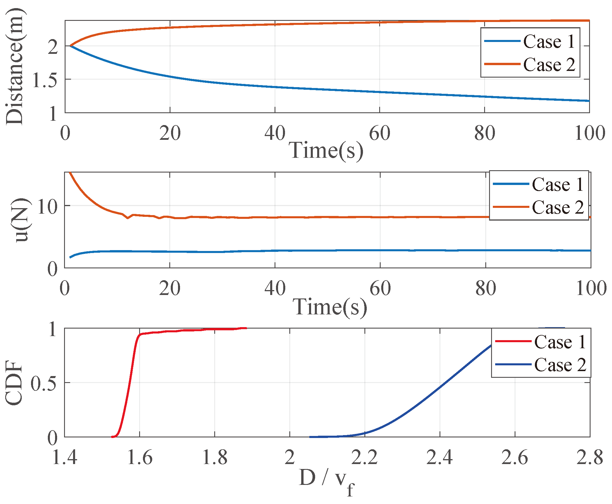
In this paper, we consider the following two cases:

Case 1: the initial velocity of the UGV is greater than that of the UAV:

As depicted in Figure 10, the UGV tends to move away from the UAV. To close the distance gap while ensuring that the Armor imaging remains sufficiently large in the frame, the UAV increases its speed to catch up with the UGV. In the initial 0–10 s, the UAV’s velocity, denoted as ${\mathit{v}}_f$, exponentially increases as it swiftly narrows the gap with the UGV. Between 20 and 60 s, ${\mathit{v}}_f$ gradually aligns with the UGV’s velocity, denoted as ${\mathit{v}}_l$, and achieves stability. After 60 s, ${\mathit{v}}_f$ and ${\mathit{v}}_l$ essentially equalize. Figure 11 (top) illustrates that the distance between the UAV and UGV stabilizes at a value not exceeding 2.4 m. Meanwhile, Figure 11 (bottom) presents the cumulative distribution function (CDF) of $\mathit{D}/{\mathit{v}}_f$, indicating that the UAV can catch up with the UGV within ${\tau }_1$. This constraint naturally regulates the UAV’s horizontal speed to ensure the continuous tracking of the UGV.

Case 2: the initial velocity of the UAV is less than that of the UGV:

As is shown in Figure 10, the UGV tends to move closer to the UAV. To increase the distance while preserving the integrity of the Armor imaging in the entire image and avoid scenarios where it becomes unrecognizable, the UAV decreases its velocity. In the initial 0–10 s, ${\mathit{v}}_f$ exponentially decreases as the UAV slows down to match the UGV’s pace. Between 20 and 60 s, the UAV’s velocity gradually aligns with the UGV’s velocity and stabilizes. After 60 s, ${\mathit{v}}_f$ and ${\mathit{v}}_l$ essentially become consistent, achieving the desired speed. Figure 11 indicates that the distance between the UAV and UGV stabilizes at a value not less than 1 m, while Figure 11 (bottom) displays the CDF of $\mathit{D}/{\mathit{v}}_f$, demonstrating that the UAV can catch up with the UGV within ${\tau }_2$.

4. Conclusions

This study explores the prospects of a decentralized control system through the integration of UAVs and UGVs in cooperative unmanned systems. The deployment of a decentralized control system, featuring the proposed CBF–CLF strategy, not only presents but also rigorously tests a method that substantially improves the operational safety and efficiency of the UAV swarm. Through the implementation of the ICF for the cooperative systems in real-time control adjustments, our proposed algorithm enables UAVs to operate independently. Additionally, the CBF–CLF strategy plays a crucial role in ensuring safety by automatically adjusting to keep the UAVs at safe distances from the UGVs. Extensive simulations across numerous real-world scenarios have proven the reliability of the proposed system and demonstrated its potential for extensive use in diverse UAV operational applications.

In future research, we could explore the application of anti-saturation fixed-time attitude tracking control in the cooperative systems to address the input saturation issues and ensure system stability. This approach integrates low-computation learning techniques to mitigate the impact of saturation and uncertainties. By incorporating anti-saturation fixed-time attitude tracking control into the cooperative systems, we can investigate its effectiveness in enhancing the control performance, robustness, and resilience against external disturbances.

References

- Alsamhi, S.H.; Shvetsov, A.V.; Kumar, S.; Shvetsova, S.V.; Alhartomi, M.A.; Hawbani, A.; Rajput, N.S.; Srivastava, S.; Saif, A.; Nyangaresi, V.O. UAV computing-assisted search and rescue mission framework for disaster and harsh environment mitigation. Drones 2022, 6, 154. [Google Scholar] [CrossRef]
- Wang, Y.; Chen, W.; Luan, T.H.; Su, Z.; Xu, Q.; Li, R.; Chen, N. Task offloading for post-disaster rescue in unmanned aerial vehicles networks. IEEE/ACM Trans. Netw. 2022, 30, 1525–1539. [Google Scholar] [CrossRef]
- De Almeida Barbosa Franco, J.; Domingues, A.M.; de Almeida Africano, N.; Deus, R.M.; Battistelle, R.A.G. Sustainability in the civil construction sector supported by industry 4.0 technologies: Challenges and opportunities. Infrastructures 2022, 7, 43. [Google Scholar] [CrossRef]
- Niu, G.; Yang, Q.; Gao, Y.; Pun, M.O. Vision-based autonomous landing for unmanned aerial and ground vehicles cooperative systems. IEEE Robot. Autom. Lett. 2021, 7, 6234–6241. [Google Scholar] [CrossRef]
- Motlagh, N.H.; Taleb, T.; Arouk, O. Low-altitude unmanned aerial vehicles-based internet of things services: Comprehensive survey and future perspectives. IEEE Internet Things J. 2016, 3, 899–922. [Google Scholar] [CrossRef]
- Galar, D.; Kumar, U.; Seneviratne, D. Robots, Drones, UAVs and UGVs for Operation and Maintenance; CRC Press: Boca Raton, FL, USA, 2020. [Google Scholar]
- Liang, X.; Zhao, S.; Chen, G.; Meng, G.; Wang, Y. Design and development of ground station for UAV/UGV heterogeneous collaborative system. Ain Shams Eng. J. 2021, 12, 3879–3889. [Google Scholar] [CrossRef]
- Chen, J.; Zhang, X.; Xin, B.; Fang, H. Coordination between unmanned aerial and ground vehicles: A taxonomy and optimization perspective. IEEE Trans. Cybern. 2015, 46, 959–972. [Google Scholar] [CrossRef]
- Gupta, A.; Fernando, X. Simultaneous localization and mapping (slam) and data fusion in unmanned aerial vehicles: Recent advances and challenges. Drones 2022, 6, 85. [Google Scholar] [CrossRef]
- Miki, T.; Khrapchenkov, P.; Hori, K. UAV/UGV autonomous cooperation: UAV assists UGV to climb a cliff by attaching a tether. In Proceedings of the 2019 International Conference on Robotics and Automation (ICRA), IEEE, Montreal, QC, Canada, 20–24 May 2019; pp. 8041–8047. [Google Scholar]
- Bianchi, M.; Barfoot, T.D. UAV localization using autoencoded satellite images. IEEE Robot. Autom. Lett. 2021, 6, 1761–1768. [Google Scholar] [CrossRef]
- Wilson, A.; Kumar, A.; Jha, A.; Cenkeramaddi, L.R. Embedded sensors, communication technologies, computing platforms and machine learning for UAVs: A review. IEEE Sens. J. 2021, 22, 1807–1826. [Google Scholar] [CrossRef]
- Wang, X.; Pan, H.; Guo, K.; Yang, X.; Luo, S. The evolution of LiDAR and its application in high precision measurement. In Proceedings of the IOP Conference Series: Earth and Environmental Science, Beijing, China, 18–20 November 2019; Volume 502, p. 012008. [Google Scholar]
- Sinfield, J.V.; Fagerman, D.; Colic, O. Evaluation of sensing technologies for on-the-go detection of macro-nutrients in cultivated soils. Comput. Electron. Agric. 2010, 70, 1–18. [Google Scholar] [CrossRef]
- Minaeian, S.; Liu, J.; Son, Y.J. Vision-based target detection and localization via a team of cooperative UAV and UGVs. IEEE Trans. Syst. Man Cybern. Syst. 2015, 46, 1005–1016. [Google Scholar] [CrossRef]
- Yang, Q.; Shi, L.; Han, J.; Yu, J.; Huang, K. A near real-time deep learning approach for detecting rice phenology based on UAV images. Agric. For. Meteorol. 2020, 287, 107938. [Google Scholar] [CrossRef]
- Wang, D.; Li, W.; Liu, X.; Li, N.; Zhang, C. UAV environmental perception and autonomous obstacle avoidance: A deep learning and depth camera combined solution. Comput. Electron. Agric. 2020, 175, 105523. [Google Scholar] [CrossRef]
- Shrestha, A.; Mahmood, A. Review of deep learning algorithms and architectures. IEEE Access 2019, 7, 53040–53065. [Google Scholar] [CrossRef]
- Zhang, F.; Yu, J.; Lin, D.; Zhang, J. UnIC: Towards unmanned intelligent cluster and its integration into society. Engineering 2022, 12, 24–38. [Google Scholar] [CrossRef]
- Behjat, A.; Manjunatha, H.; Kumar, P.K.; Jani, A.; Collins, L.; Ghassemi, P.; Distefano, J.; Doermann, D.; Dantu, K.; Esfahani, E.; et al. Learning robot swarm tactics over complex adversarial environments. In Proceedings of the 2021 IEEE International Symposium on Multi-Robot and Multi-Agent Systems (MRS), Cambridge, UK, 4–5 November 2021; pp. 83–91. [Google Scholar]
- Ruan, L.; Li, G.; Dai, W.; Tian, S.; Fan, G.; Wang, J.; Dai, X. Cooperative relative localization for UAV swarm in GNSS-denied environment: A coalition formation game approach. IEEE Internet Things J. 2021, 9, 11560–11577. [Google Scholar] [CrossRef]
- Montecchiari, L. Hybrid Ground-Aerial Mesh Networks for IoT Monitoring Applications: Network Design and Software Platform Development. 2023. Available online: https://amsdottorato.unibo.it/10952/ (accessed on 20 June 2023).
- Mammarella, M.; Comba, L.; Biglia, A.; Dabbene, F.; Gay, P. Cooperative agricultural operations of aerial and ground unmanned vehicles. In Proceedings of the 2020 IEEE International Workshop on Metrology for Agriculture and Forestry (MetroAgriFor), Trento, Italy, 4–6 November 2020; pp. 224–229. [Google Scholar]
- Wu, Y.; Wu, S.; Hu, X. Cooperative path planning of UAVs & UGVs for a persistent surveillance task in urban environments. IEEE Internet Things J. 2020, 8, 4906–4919. [Google Scholar]
- Phan, C.; Liu, H.H. A cooperative UAV/UGV platform for wildfire detection and fighting. In Proceedings of the 2008 IEEE Asia Simulation Conference-7th International Conference on System Simulation and Scientific Computing, Beijing, China, 10–12 October 2008; pp. 494–498. [Google Scholar]
- Harik, E.H.C.; Guérin, F.; Guinand, F.; Brethé, J.F.; Pelvillain, H. UAV-UGV cooperation for objects transportation in an industrial area. In Proceedings of the 2015 IEEE International Conference on Industrial Technology (ICIT), Seville, Spain, 17–19 March 2015; pp. 547–552. [Google Scholar]
- Arbanas, B.; Ivanovic, A.; Car, M.; Orsag, M.; Petrovic, T.; Bogdan, S. Decentralized planning and control for UAV–UGV cooperative teams. Auton. Robot. 2018, 42, 1601–1618. [Google Scholar] [CrossRef]
- Kshemkalyani, A.D.; Singhal, M. Distributed Computing: Principles, Algorithms, and Systems; Cambridge University Press: Cambridge, UK, 2011. [Google Scholar]
- Haeberlen, A.; Kouznetsov, P.; Druschel, P. PeerReview: Practical accountability for distributed systems. ACM SIGOPS Oper. Syst. Rev. 2007, 41, 175–188. [Google Scholar] [CrossRef]
- Grocholsky, B.; Bayraktar, S.; Kumar, V.; Pappas, G. Uav and ugv collaboration for active ground feature search and localization. In Proceedings of the AIAA 3rd “Unmanned Unlimited” Technical Conference, Workshop and Exhibit, Chicago, IL, USA, 20–23 September 2004; p. 6565. [Google Scholar]
- Jayavelu, S.; Kandath, H.; Sundaram, S. Dynamic area coverage for multi-UAV using distributed UGVs: A two-stage density estimation approach. In Proceedings of the 2018 Second IEEE International Conference on Robotic Computing (IRC), Laguna Hills, CA, USA, 31 January–2 February 2018; pp. 165–166. [Google Scholar]
- Casbeer, D.W.; Beard, R. Distributed information filtering using consensus filters. In Proceedings of the 2009 IEEE American Control Conference, St. Louis, MO, USA, 10–12 June 2009; pp. 1882–1887. [Google Scholar]
- Omotuyi, O.; Pokhrel, S.; Sharma, R. Distributed quadrotor uav tracking using a team of unmanned ground vehicles. In Proceedings of the AIAA Scitech 2021 Forum, Virtual, 11–15 & 19–21 January 2021; p. 0266. [Google Scholar]
Figure 1.
The schematic diagram of UAV–UGV cooperative system.
Figure 2.
Armor (light bars are the main visual features; A, B, C, and D are four points used for solving pose).
Figure 3.
Geometric structure of PNP.