
Impact Analysis of Time Synchronization Error in Airborne Target Tracking Using a Heterogeneous Sensor Network


1
Department of Mechanical Engineering, Chung-Ang University, Seoul 06974, Republic of Korea
2
School of Aerospace, Manufacturing and Transport, Cranfield University, Bedford MK43 0AL, UK
3
Cho Chun Shik Graduate School of Mobility, Korea Advanced Institute of Science and Technology, Daejeon 34141, Republic of Korea
*
Author to whom correspondence should be addressed.
Drones 2024, 8(5), 167; https://doi.org/10.3390/drones8050167
Submission received: 5 March 2024
/
Revised: 8 April 2024
/
Accepted: 16 April 2024
/
Published: 23 April 2024
(This article belongs to the Special Issue Advances in Detection and Tracking Applications for Drones and UAM Systems)
Abstract
:This paper investigates the influence of time synchronization on sensor fusion and target tracking. As a benchmark, we design a target tracking system based on track-to-track fusion architecture. Heterogeneous sensors detect targets and transmit measurements through a communication network, while local tracking and track fusion are performed in the fusion center to integrate measurements from these sensors into a fused track. The time synchronization error is mathematically modeled, and local time is biased from the reference clock during the holdover phase. The influence of the time synchronization error on target tracking system components such as local association, filtering, and track fusion is discussed. The results demonstrate that an increase in the time synchronization error leads to deteriorating association and filtering performance. In addition, the results of the simulation study validate the impact of the time synchronization error on the sensor network.
1. Introduction
The use of unmanned aerial vehicles (UAVs) has attracted much attention in a broad range of applications. However, the ubiquitousness of UAVs in the airspace has introduced new risks arising from their potential misuse. For example, a drone intrusion disrupted Gatwick airport in December 2018, leading to a 33-h closure which resulted in an estimated loss of GBP 50 million [1]. These increased risks have necessitated the development of counter-unmanned aerial systems (CUAS) to identify UAVs, monitor their behaviors, and implement appropriate countermeasures. A CUAS typically deploys multiple heterogeneous sensors to accurately and promptly detect, identify, and collect target information for surveillance [2,3,4]. The distributed target data are then aggregated at the fusion center. In the sensor fusion process, a common notion of time across the sensors is essential, as correlations between the collected data are evaluated based on time information [5]. Therefore, tight synchronization across the heterogeneous sensor network is necessary to improve target tracking and sensor fusion.
Time synchronization aims to provide a common time shared between local sensors with unsynchronized clocks, thereby ensuring that all nodes in the sensor network are in alignment with a timing reference. Synchronization based on the global navigation satellite system (GNSS) is a typical solution, in which accurate time sources from satellites are used as the reference timing. In the context of time distribution, one-pulse-per-second (1-PPS) synchronizing signals from global positioning system (GPS) or GNSS receivers or synchronization protocols [6,7,8,9,10,11,12,13,14,15,16,17,18] allow local sensors to be aligned across the network through communication [17]. Although synchronization directly through GNSS clocks facilitates the realization of precise time accuracy, it requires additional equipment with access to the satellite signal from all local sensors. Time synchronization protocols are developed in order to distribute time over packet-switched networks and to synchronize distributed devices such as the network time protocol (NTP) [12] and precision time protocol (PTP) [13] for time-sensitive networking (TSN). Wireless TSN frameworks, such as reference broadcast synchronization (RBS) and time synchronization protocol for sensor networks (TPSN), have been developed as well [9,11,18]. However, GNSS-based synchronization relies on the GNSS system, and may be vulnerable to system failure, environmental interference such as urban canyons, and intentional disruptions such as jamming or spoofing with time error injection [7]. For example, in January 2021 GPS was noted to be unreliable within a 50-nautical-mile radius of the Denver International Airport, which caused disruptions to infrastructure and air traffic management applications. The incident lasted for 33 h, which led to drifting of the clocks for each subsystem during the disruption and caused the ground control station to become isolated [19]. To address concerns regarding GNSS reliability, it is necessary to use timing systems that do not directly rely on local GNSS receivers. An alternative is to use fault-tolerant clock synchronization based on redundant clock sources [8,9,10] or receiver-independent time synchronization [20].
Considering the importance of time synchronization in target tracking, it is essential to understand the potential correlation between time synchronization and target tracking performance. However, the existing studies have not extensively explored the effects of time synchronization. Typically, time synchronization and target tracking systems in sensor networks are designed independently. Previous studies have demonstrated that synchronization accuracy is influenced by several factors, including the quality of the clock source, the timestamp resolution, and the network topology. Additionally, characteristics of sensors such as radar, acoustic sensors, and cameras as well as their deployment in diverse environmental conditions, e.g., operations with various temperatures, and density or tracking systems applied to different domain such as underwater or aerial vehicles, can contribute to time synchronization errors [21]. A time synchronization protocol is typically established to meet a specified precision level, while target tracking systems are developed assuming that the time information is sufficiently accurate. Various filtering schemes aimed at improving state estimation in the presence of delayed measurements have been proposed [22,23,24], primarily focusing on state estimation within the target tracking system. In a target tracking system employing multiple sensors, data association and state estimation within the sensor fusion rely on temporal information from local sensors. In this regard, any imprecision in the time alignment among sensors can adversely affect these processes, leading to inconsistencies and compromised reliability in data fusion. Nevertheless, the influence of time synchronization errors on the target tracking system remains to be clarified. In light of the heightened demand for advanced tracking precision, particularly in the context of proximity operations for UAVs navigating dense urban environments, it is necessary to examine correlations between errors resulting from loose time synchronization and the overall performance of the target tracking system.
Therefore, the objective of this work is to investigate the impact of time synchronization errors on the performance of sensor fusion and target tracking. The target tracking system considered in this study consists of two system layers: a sensing layer using heterogeneous local sensors and a data processing and tracking layer located at the fusion center (FC). Similar to networked components, clocks are mathematically modeled in a linear form. The reference clock is accurate in the FC, while a time offset is assumed for each local clock to introduce errors to the timing in the network. Clock synchronization is assumed to occur when the time error between the local clock and the reference is within a predefined accuracy threshold, while time synchronization fails when the time error exceeds the threshold. Additionally, the influence of the time synchronization error on target tracking system components, such as local association, filtering, and track fusion, is discussed in order to clarify the correlation between the time error and the tracking performance. A simulation study is performed to validate the analytical results. Our findings indicate that the target tracking system performance can deteriorate due to increasing time synchronization errors. Notably, the system performance is evaluated against a number of target tracking performance metrics, including the root mean square error (RMSE), generalized optimal sub-pattern assignment (GOSPA) [25], and single integrated air picture (SIAP) [26].
The main contribution of this study lies in a systematic assessment of the influence of time synchronization errors on sensor fusion in target tracking systems. We design a sensor fusion system model that reflects time synchronization errors across sensor networks. Track-to-track fusion (T2TF) with time alignment in the local tracker is introduced to handle heterogeneous sensor characteristics. Moreover, we investigate the influence of time synchronization on individual components of the sensor fusion system, including filtering, association, and track fusion processes. Our analysis reveals observable performance degradation in terms of bias and error covariance. These findings suggest that the sensor fusion system experiences significant impairment when synchronization errors become non-negligible. Our simulation study provides empirical results illustrating the impact of synchronization errors on tracking performance. These insights can help to mitigate potential issues in target tracking systems that rely on sensor networks as well as in other network systems that require time synchronization [27,28].
The remainder of this paper is organized as follows: Section 2 details the time synchronization process and synchronization error considered in this study; Section 3 explains the target tracking system and sensor fusion technique; Section 4 discusses the influence of the time synchronization error on the target tracking system components; Section 5 presents the results of our numerical simulation; and Section 6 presents concluding remarks and recommendations for further work.
2. Preliminaries
This section introduces the time synchronization method using two-way communication and the time error model considered in this study. Figure 1 illustrates the network topology considered in this study, in which all sensor nodes are fully connected to a central node. The command and control (C2) serves as the central node; the server clock in C2 has access to a precision reference clock from a terrestrial source, serving as an alternate position, navigation, and timing (PNT) reference [10,17].
We assume that the server clock is accurate and serves as the reference clock . The local clock time can be expressed in the following first-order affine form [11]:
where the subscripts a and p represent active and passive sensor nodes, respectively, and is the time error, which can be time-varying as follows:
where refers to the clock drift due to frequency mismatch, refers to the previous synchronization time instance, is the initial offset calculated at , and contributes to stochastic uncertainties, including unmodeled errors. The drift coefficient indicates the increasing time error over time. Considering a worst-case scenario, we assume that the drift for active sensor is negative while that for passive sensor is positive. To synchronize slave clocks to the server, the server clock time is distributed to the slave clocks over a communication network and the local clock adjusts its offset as follows:
where is the approximate offset to be determined. The synchronization accuracy determines the error magnitude. Several synchronization protocols standardize the accuracy requirement [12,13], and synchronization procedures have been developed to achieve the synchronization requirements over the networks [14,15,16]. However, the time synchronization performance in practical applications may be impaired by various factors, such as GNSS receiving failures or variable and asymmetric latencies [29]. To address this issue, viable failover solutions are required in order to ensure resilient reference timing distributions. In these instances, an accurate time source is distributed to the network server to ensure that time error is maintained within the required offset bound . Similarly to the approach presented in [30,31,32], we conducted hardware experiments to obtain statistical results of time errors, for which the distribution is modeled as a normal distribution:
where and are the mean and standard deviation, respectively, and are set to 422 μs and 62.293 μs following experimental results. The required offset bound is set to ms for the worst-case analysis. In the worst-case scenario involving the largest time variation between local clocks, two synchronized clocks can drift from each other at a rate of at most , where . The time difference between node clocks is expressed as
To limit the relative offset to , the maximal holdover interval should be bounded as
If the local clocks are not synchronized, clock skew increases the time difference from the reference value during holdover. If the holdover period is longer than (6), then the time synchronization error exceeds the requirement. The synchronization error due to longer holdover periods is discussed in Section 4.
3. Target Tracking System
Figure 2 illustrates the target tracking system structure explored in this study. The sensing layer exchanges data with the tracking and data fusion layer through network communication. The sensing layer consists of active and passive sensors. Sensors are distributed on the surveillance site to detect target signals. The target measurements are timestamped by the local clock and sent to the tracking and fusion layer through the communication network. The tracking and fusion layer possesses a main sensor fusion architecture based on T2TF, wherein a local tracker processes target measurements into local tracks which are then integrated into fused tracks via track fusion. Notably, T2TF enables more effective data transmission through network communication than the measurement-to-track structure, and as such has found wide application [33,34,35,36]. Local measurements are first processed at local trackers to estimate and predict tracks. The FC placed at the end of the data process aggregates the local tracks and fuses them into central tracks. The heterogeneous T2TF algorithm based on practical decomposition [37] helps to associate local tracks with different dimensions and synthesize them into a global track. The update rates in the tracking and data fusion layer and active sensor are synchronous, while the update rates in the passive sensor are two times smaller than those in other modules. The clock in the tracking and fusion layer is assumed to be synchronized to GNSS and can serve as a reference clock or server clock.
3.1. Sensor Model
In the sensing layer, two heterogeneous sensors are used, i.e., active radar and passive radio frequency (RF) sensors, in light of their widespread adoption in CUAS surveillance systems [4,38,39,40]. The radar sensor provides target position measurements, whereas the RF sensor passively detects target position only in two-dimensional space. The two sensors are asynchronous, with the passive sensors having a smaller update rate than the active sensor. The radar periodically scans a search space with sampling time . In the k-th scan period, the radar may detect a target at and record the detected measurement timestamped using the current local time . The measurement in vector form can be expressed as follows:
where represents the target range, azimuth, and elevation angles expressed in the spherical coordinate system. Suppose that a target and the radar are located at and , respectively; then, the measurement variables exhibit the following relationships:
The measurement is performed until the scanning is complete and then transmitted to the local tracker through the network at , which inevitably introduces a time delay .
In contrast, the RF sensor takes only the target measurement expressed in two-dimensional space. Let be the sampling time for the RF sensor, which is larger than that of the radar, i.e., . The RF measurement can be expressed in vector form as follows:
If the RF sensor is located at , then the measurements can be rewritten in terms of the relative positions with the target:
The detected target measurements are sent to each local tracker in the tracking and fusion layer through the network. Table 1 summarizes the sensor specifications considered in this study.
3.2. Local Tracker
In the local tracker, sensor measurements received from local sensors are processed as local tracks. The state-space model is defined as
Depending on the sensor measurement, the local tracker exhibits different state and measurement variables, i.e., and , respectively. To simplify the notation, the current time step of the tracker is denoted by k and variables evaluated at are expressed with the subscript k. Each local tracker uses the association function to perform measurement-to-track association and performs filtering to estimate target states with time alignments of the measurement timestamp to the evaluation period. Association requires the discrimination of target measurements from clutter; the aim of the filtering process is to appropriately estimate the target states. At time step k, measurements taken at are timestamped as , which may lie in the track interval . Therefore, it is necessary to perform time alignment in order to address the time mismatch between measurements and the track time calculated according to the reference clock.
This study adopts the standard extended Kalman filter (EKF) technique [41] to estimate local track states in the presence of asynchronous timing between the measurement and track. Specifically, we include an intermediate time index in the track interval to define two sub-intervals and . Here, corresponds to the time instant at which the target measurement is obtained, i.e., .
3.2.1. Measurement-to-Track Association and Filtering
In the first period , a posteriori state estimates and covariance matrix, i.e., and at , respectively, are obtained using the standard EKF procedure. The target tracking algorithm in this period consists of a priori and measurement updates with measurement-to-track association. In the state prediction step, the track states in the previous step are predicted up to measurement update step to obtain a priori estimates. Let be the track estimates in the previous step. Using Equation (11), the a priori estimates and covariance matrix approximation using a linear model can be obtained as follows:
where represents the Jacobian matrix of the state transition function and is the process noise covariance matrix propagated from to .
At measurement update step , the standard EKF updates states and covariance matrix approximation are
where denotes the innovation term for measurement updates, is the Kalman gain, and is the innovation matrix. In a cluttered environment, multiple measurements may be mixed with actual data from the target and incorrect data resulting from noise or false alarms; therefore, it is necessary to distinguish correct target measurements from spurious data. In this study, a probabilistic approach using a joint probability data association (JPDA) algorithm is used [42,43,44]. The predicted measurement and covariance of innovation are obtained as follows:
where denotes the Jacobian matrix of the observation function. The association test between the predicted measurement and observations is performed by measuring the statistical distance
where is the total number of measurements. The set of validated measurements is defined as
where is the number of validated measurements in step k. The posterior probability distribution of each target obtained from the JPDA filter is a Gaussian mixture distribution. The state estimation is updated using a pseudo-innovation term
e.g., a weighted sum of the original innovation terms, where represents the marginal association probability from measurement j and is the predicted measurement track. Next, the pseudo-innovation term is applied to the standard EKF in the measurement update stage as follows:
where and
For track maintenance, history-based logic is used; in other words, a tentative track is confirmed to be a track if it is associated with at least one measurement N times out of M consecutive steps, while a confirmed track is eliminated if association fails n times out of m steps.
3.2.2. Track Update with Time Alignment
Considering the time discrepancy between the evaluation for estimation and the measurement timestamped , the measurement can be regarded as a delayed detection. In the second period [, a track update is performed using state prediction to time step k. For track fusion, all tracks must be evaluated at the same time in order to perform T2TF. Because each local tracker updates its measurement at , the posteriori should be further propagated such that all local tracks have the same time alignment. The main objective of the track update is to obtain the state prediction and covariance values, respectively and :
Notably, the large amount of clock offset due to synchronization failure may involve a measurement time step that is far from the current track interval. If the negative time offset involves for , then the measurements can be regarded as out-of-sequence measurements (OOSMs) such that the measurements obtained in the previous interval correspond to the current time step k. In this case, the OOSMs can be handled based on the approach presented in [45,46]. First, we consider the state estimates at k. The track automatically traverses the states and covariance from k − 1 to k and , as no measurement exists in the current update interval . In the retrodiction step, the current state and covariance are propagated back from k to :
where represents the backward state transition matrix from k to , is the covariance matrix for the process noise, and is defined as
In the second step, retro-correction is performed to correct the current state and state covariance using the OOSMs with a JPDA algorithm. The Kalman gain and innovation matrix at time step can be rewritten as
where is the observation Jacobian matrix and is the covariance matrix for the OOSMs. Now, the corrected state can be derived as follows:
where and
In contrast, a large positive time offset may involve . Because the tracker can only process measurement times smaller than the current time, the invalid measurement is intentionally delayed up to one step to ensure that it can be suitably processed.
3.3. Track Fusion
When the FC receives local tracks, the tracks are fused through track fusion to produce global tracks. Because local tracks have different state-space models with different dimensions, i.e., and , the association must be performed only on their shared state space. This study adopts a practical T2TF technique [37]. Track association first compares local tracks through the statistical association test. Considering the mapping , the state vector of the active sensor track can be partitioned as , where and are partitioned state vectors. The corresponding covariance matrix and can be expressed as
Based on the partition, the association test validates the statistical closeness between two tracks through comparison with the gating threshold:
where b is the gating threshold. If the hypothesis is validated, the two tracks can be fused using the intersection method [47]:
where represents a weight parameter chosen from within . After fusion in the shared state space, the complement state is added from the active sensor track as
4. Impact Analysis
4.1. Influence on Local Tracking and Association
The local tracker accommodates inaccurate measurement time information and may corrupt estimated tracks, thereby adversely influencing the estimation accuracy and association consistency. This section discusses the influence of the time error on the local tracking process. Here, is the ideal time index at which the measurement is taken, while represents the variables for the ideal case with .
4.1.1. Influence on Measurement-to-Track Association and Filtering
In phase , the time error may influence the association and filtering processes. For association, the predicted measurement track and covariance matrix should be propagated from the previous time step to . Supposing that the local track in the previous step is accurate and that the relation
is satisfied, then, considering the time error , the update interval for measurement prediction satisfies . The deviation between the predicted measurements and covariance for ideal and corrupted tracks are
where denotes the 2-norm and is the state transition error matrix. Equation (32) indicates that the predicted measurement error from the ideal case increases with respect to as it is amplified by . In turn, the incorrect measurement prediction affects the estimation accuracy. Furthermore, the covariance of innovation matrix can be defined as
Equation (33) reflects that the update to the innovation is minor in the corrupted track case. The small innovation update affects the association test, i.e.,
which may imply that the statistical distance with the same deviation between the actual measurement and prediction becomes significant with . This may lead to unsuccessful validation of the target measurement and deteriorate the consistency of the track association. In addition to the propagation error associated with kinematic mismatch and process error, the prediction error worsens as well.
4.1.2. Influence on Track Update with Time Alignment
In the track update phase, the updated track may be corrupted by the inaccurate update interval between and k. For simplicity, suppose that the synchronization error is negative and that the target measurement is validated as . The measurement update step corrects the state estimates and covariance matrix using latest measurement at . Given this information, we assume that the a posteriori estimates and covariance matrix are similar to those of the ideal case, as
Now, the track update propagates the posteriori to the current time k. According to Equation (19), the estimation error from ideal estimates satisfies
Equation (36) indicates that the deviation from the ideal track increases by . In particular, propagates the track further along the target velocity direction when . Furthermore, the covariance matrix can be written as
which means that the covariance grows as the time error acts on the local measurement. In turn, the prediction step for time alignment leads to deviation of the state estimates from the actual target, and this trend becomes more pronounced as the time offset increases.
4.2. Impact on Track-to-Track Association
As described in Section 4.1, the time synchronization error increases the tracking error and error covariance in local tracks. A larger time error leads to increased error covariance from the local filter, and the fused covariance is affected as well; therefore, the time error results in tracking degradation. In addition, the degraded quality of local tracks can affect the track-to-track association. The increase in time error reflects the deviation between the local track estimates and the reduced association between local tracks. Suppose that two local sensors detect the target at with different timestampings by local clocks; let and denote the measurement time steps corrupted by inaccurate local clocks. Then, Equation (36) yields
Considering the maximum time deviation between local clocks (9), the deviation between local tracks can be expressed as
Equation (39) implies that the deviation increases as amplifies the upper bounds between local tracks.
5. Simulation Study
Numerical simulations were performed to validate the impact analysis. We considered the scenario of an intruder drone being detected near an airport, as shown in Figure 3. The target is moving from with constant velocity . The radar is located at the center of the surveillance space, and is capable of 360-degree field of view functionality through the use of a rotating receiver antenna, while the RF sensors are distributed to continuously search the space. The sensor detects the target in the cluttered environment, and local trackers process the cluttered measurements and generate local tracks. The RF tracker receives measurements from the RF sensor once in two cycles. The tracker coasts the track alternately when the measurement is not transmitted. MATLAB Sensor Fusion Toolbox was used to model the sensors [48], and the sensor specifications and system parameters are summarized in Table 2.
For clock offsets, we consider the worst-case scenario, where the radar clock has negative time offset and the RF sensor has positive time offset. The local clocks are considered to be synchronized when the clock offsets are bounded below the criterion under the required accuracy ms, which is obtained from the statistical model (Equation (4)). Otherwise, the networks are unsynchronized. The time offsets are increased to monitor the qualitative trends of the performance with respect to the time error.
The performance is evaluated using three metrics. The average RMSE refers to the localization error of the track result compared with the ground truth. Lower RMSE scores correspond to higher tracking precision. In this study, the RMSE criterion is set as 2 m.
The GOSPA [25] is used to assess the tracking performance by simultaneously considering track completeness in terms of the localization error, miss target, and false tracks.
Lastly, we consider the single integrated air picture (SIAP) [26], which helps to separately examine the tracking quality in terms of consistency and correctness. This metric includes two metrics; the Completeness indicates the percentage of number of tracked targets to the number of actual targets related to missed targets, while the Spuriousness is the percentage of the number of false tracks out of the number of total tracks.
5.1. Comparison between Synchronized and Unsynchronized Sensor Networks
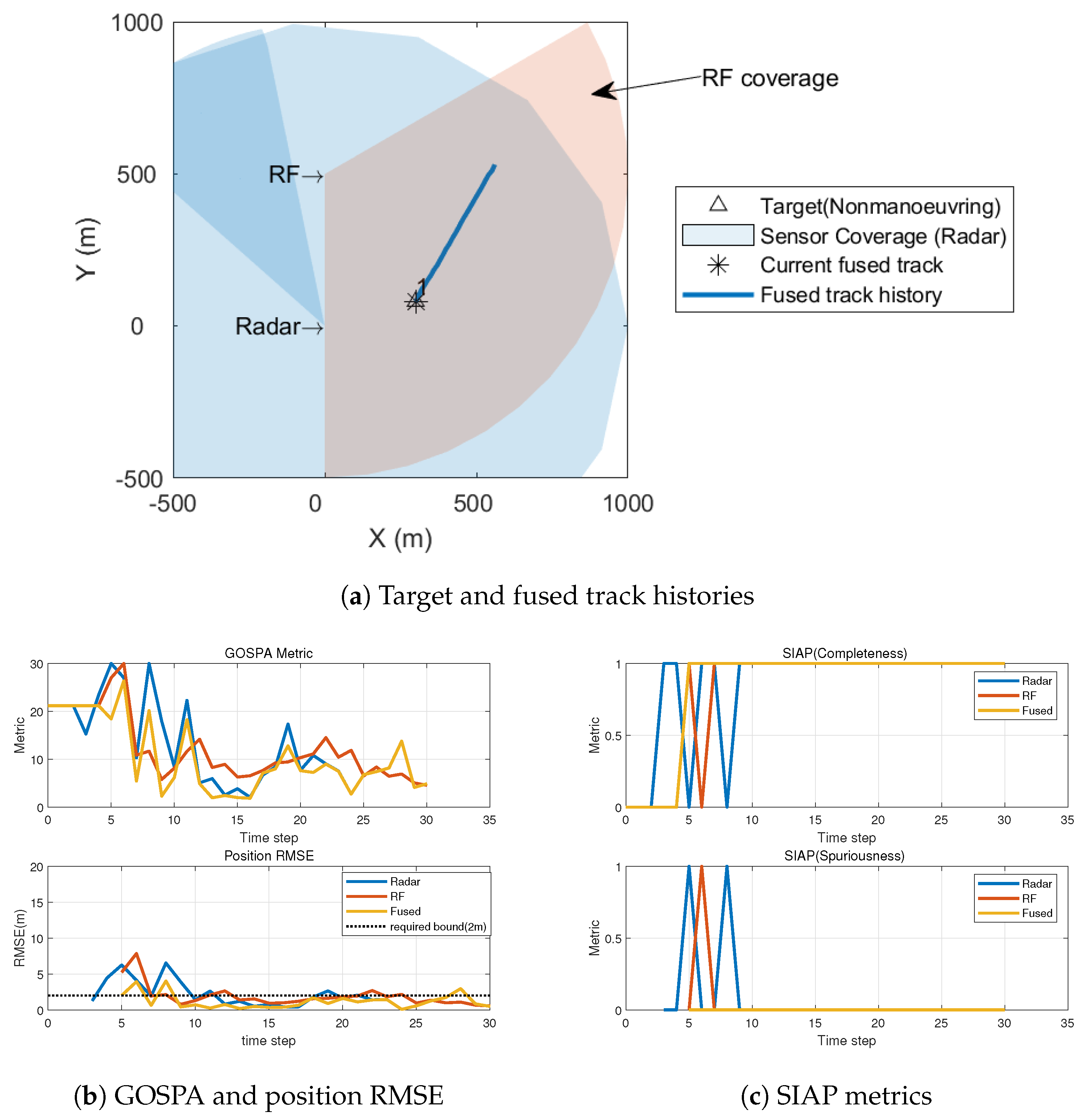
Figure 4 shows the target tracking results when the sensors are time-synchronized under the required precision ms. The track trajectory, presented in an identical color in Figure 4a, indicates that the fused track is consistently derived during the scenario. As shown in Figure 4b, the confirmation times in local and fused tracks are different. The radar track is confirmed at the third time step, while the RF tracker confirms its local track at the fifth time step when the measurement arrives three times. Finally, the fused track is derived from the fifth time step when two local tracks are confirmed. Local tracks exhibit large tracking errors and missed targets in a few initial steps, while the fused track exhibits improved tracking accuracy. Table 3 summarizes the performance measures. Compared with the ideal case without any time error, the overall target tracking performance is maintained within satisfactory limits.
In contrast, the target tracking system exhibits reduced performance in the unsynchronized sensor network. Figure 5 shows that each local tracker generates a local track but displays large tracking errors when a significant time error ( s) is imposed on the local clocks. Time alignment in track update causes the track to deviate from the measurements, introducing a large RMSE. Consequently, the completeness metric reflects that the track is not correctly assigned to the target and labels it as a false track. Furthermore, the track fusion is significantly impaired. The RMSE significantly increases and exceeds the tracking requirement. In addition, the consistency of the fused track deteriorates in most of the time intervals. Figure 5a illustrates that the fused track trajectory is not consistent. From the fifth to tenth time steps, the fusion center cannot fuse the two local tracks and yields two separate tracks, potentially because of the enlarged error bound in Equation (39) as the time error increases. This result indicates that the tracking performance is significantly affected by the time error when the local clocks are no longer synchronized.
5.2. Performance under Increasing Synchronization Errors
To examine the influence of the synchronization error on the target tracking system, we implemented the same tracking scenario with synchronization errors increasing from the zeroth time step to the first. Figure 6 plots the average values of the performance measures for each episode. The local and fused tracks exhibit less sensitivity to the synchronization error when the offset is within the allowable offset ms. However, the tracking degradation becomes noticeable when the synchronization error exceeds 100 ms. Considering the clock drift during the longer holdover interval, the holdover time at which significant performance degradation is observed can be estimated. For example, local clocks with an accuracy of 2 ppm (parts per million) take h to reach the time error of 100 ms. This time is reduced for low-cost clocks due to the large frequency stability in their oscillators.
Furthermore, the fused performance worsens compared with that of local tracks in the presence of significant time errors, which implies that fusion with tracks corrupted by synchronized time errors may result in reduced tracking quality. Notably, a correlation exists between the RMSE/GOSPA and SIAP metrics; RMSE and GOSPA grow significantly after 100 ms, and and indicate that the tracking system degrades the track consistency in this period. GOSPA incorporates the missed (completeness) and false (spuriousness) components. A large RMSE indicates that the distanced track becomes less coherent from a kinematic perspective, and the corresponding association with the central track may fail, as observed in Figure 5. The exponential increase in RMSE with the log-scale temporal error indicates that the estimation errors in the local and fusion tracks tend to be linearly proportional to the time error. This result is consistent with the impact analysis. Specifically, the approximate tendency derived in Equations (32), (36) and (39) shows the linear correlation between the performance degradation and time error.
5.3. Performance When the Target Is Maneuvering
To inspect the system performance when the target is maneuvering in the presence of synchronization error, a target tracking simulation was performed by varying the target’s motion. In this scenario, the target is in constant turning motion with identical speed m/s.
Figure 7 illustrates that the negative effects of time synchronization errors on the sensor fusion performance are aggravated when model mismatch occurs due to target maneuvering. In both cases, the tracking performance degrades as the time error increases. However, the degradation is faster in the maneuvering case, as the maximum synchronization error for meeting the performance requirement is reduced. This degradation may be attributable to a mismatch between the target motion in the tracking algorithm. The local tracker estimates the target based on the constant-velocity model in the EKF phase. The model error can be propagated along with the synchronization error in track estimates, thereby influencing the association and track updates, which may worsen when a large synchronization error is involved.
5.4. Performance under Speed Variations
As shown in Figure 8a, RMSE and GOSPA increase rapidly as the target speed increases. For example, the time to reach the RMSE error of 2 m is 0.24 s when the target speed is 10 m/s, while it is significantly reduced to 0.05 s when the target speed increases to 40 m/s. This phenomenon likely occurs because the velocity components in the state vector lead to sizable spatial transitions over time. The high speed of the target potentially introduces a significant position error in Equation (36). In addition, the track consistency degrades faster as the speed increases. Moreover, when the target speed increases, the robustness of sensor fusion against the time synchronization error is reduced as the completeness metric decreases. Figure 8c shows the empirical results of the allowable synchronization errors for track consistency and estimation accuracy. The blue shaded area represents the allowable time error for guaranteed estimation accuracy, while the grey shaded area denotes the allowable region of the consistent track. Both regions narrow as the target speed increases. The estimation accuracy region is smaller than the consistent track region, indicating that the tracking requirement is considerably tighter in this scenario. The consistency region can be widened as the association threshold is adaptively set or increased.
6. Conclusions
This study aimed to examine the influence of time synchronization errors on the performance of a target tracking system. The time synchronization error was mathematically modeled and imposed on local clocks as the clock offset. The target tracking system consisted of heterogeneous sensors under a T2TF architecture. The local tracking process included a track update step for time alignment to account for the asynchronous timing between measurements and tracks and to accommodate synchronization errors in generating local tracks. The impact of the time synchronization error on association, filtering, and track fusion was considered, and empirical results were obtained through simulations. Under linear target dynamics, the synchronization error linearly degraded the tracking error, resulting in inconsistent association. Variations in other factors, including target speed and maneuvering, also led to deterioration in tracking performance owing to time synchronization errors. The simulation results demonstrated that these negative effects on the target tracking system become pronounced when the error exceeds 100 ms. These results highlight the need for a resilient synchronization system that can ensure time synchronization across the network in order to maintain synchronization errors within an acceptable accuracy level. Joint estimation of time synchronization and target position in target tracking and sensor fusion processes can be implemented to mitigate the errors when a synchronization failure occurs. The findings of this work can be extended to other sensor network systems to clarify the influence of synchronization errors and facilitate system improvements. Further research could explore the development of state estimation techniques aimed at improving tracking performance in the presence of measurement delays, with a specific focus on addressing the impact of time synchronization in sensor networks.
Author Contributions
Conceptualization, S.L., I.P. and H.S.; methodology, S.L. and H.S.; software, S.L.; investigation and validation, S.L., Z.Y. and H.S.; writing—original draft preparation, S.L.; writing—review and editing, All authors; project administration, I.P.; funding acquisition, H.S. All authors have read and agreed to the published version of the manuscript.
Funding
This work was supported by Innovate UK funding (grant number 10012306).
Data Availability Statement
Not applicable.
Conflicts of Interest
The authors declare no conflicts of interest.
References
- Hallie, D. Gatwick’s December Drone Closure Cost Airlines $64.5 million. Fortune. 2019. Available online: https://fortune.com/2019/01/22/gatwick-drone-closure-cost/ (accessed on 4 March 2024).
- Kaleem, Z.; Rehmani, M.H. Amateur Drone Monitoring: State-of-the-Art Architectures, Key Enabling Technologies, and Future Research Directions. IEEE Wirel. Commun. 2018, 25, 150–159. [Google Scholar] [CrossRef]
- Pingali, G.; Tunali, G.; Carlbom, I. Audio-visual tracking for natural interactivity. In Proceedings of the Seventh ACM iInternational Conference on Multimedia (Part 1), Orlando, FL, USA, 30 October–5 November 1999; pp. 373–382. [Google Scholar]
- Azari, M.M.; Sallouha, H.; Chiumento, A.; Rajendran, S.; Vinogradov, E.; Pollin, S. Key Technologies and System Trade-offs for Detection and Localization of Amateur Drones. IEEE Commun. Mag. 2018, 56, 51–57. [Google Scholar] [CrossRef]
- Kaempchen, N.; Dietmayer, K. Data synchronization strategies for multi-sensor fusion. In Proceedings of the IEEE Conference on Intelligent Transportation Systems, Shanghai, China, 12–15 October 2003; Volume 85, pp. 1–9. [Google Scholar]
- Chowdhury, D.D. NextGen Network Synchronization; Springer: Cham, Switzerland, 2021. [Google Scholar]
- Dana, P.H. Global Positioning System (GPS) time dissemination for real-time applications. Real-Time Syst. 1997, 12, 9–40. [Google Scholar] [CrossRef]
- Kyriakakis, E.; Tange, K.; Reusch, N.; Zaballa, E.O.; Fafoutis, X.; Schoeberl, M.; Dragoni, N. Fault-tolerant Clock Synchronization using Precise Time Protocol Multi-Domain Aggregation. In Proceedings of the 2021 IEEE 24th International Symposium on Real-Time Distributed Computing (ISORC), Daegu, Republic of Korea, 1–3 June 2021; pp. 114–122. [Google Scholar] [CrossRef]
- Seijo, O.; Iturbe, X.; Val, I. Tackling the Challenges of the Integration of Wired and Wireless TSN with a Technology Proof-of-Concept. IEEE Trans. Ind. Inform. 2021, 18, 7361–7372. [Google Scholar] [CrossRef]
- Lo, S.; Akos, D.; Dennis, J. Time Source Options for Alternate Positioning Navigation and Timing (APNT); Technical Report; Federal Aviation Administration: Washington, DC, USA, 2012.
- Lévesque, M.; Tipper, D. A survey of clock synchronization over packet-switched networks. IEEE Commun. Surv. Tutor. 2016, 18, 2926–2947. [Google Scholar] [CrossRef]
- Mills, D. Internet time synchronization: The network time protocol. IEEE Trans. Commun. 1991, 39, 1482–1493. [Google Scholar] [CrossRef]
- 1588–2019—IEEE Standard for a Precision Clock Synchronization Protocol for Networked Measurement and Control Systems; IEEE: New York, NY, USA, 2020; pp. 1–499. [CrossRef]
- Wang, H.; Shao, L.; Li, M.; Wang, B.; Wang, P. Estimation of Clock Skew for Time Synchronization Based on Two-Way Message Exchange Mechanism in Industrial Wireless Sensor Networks. IEEE Trans. Ind. Inform. 2018, 14, 4755–4765. [Google Scholar] [CrossRef]
- Xiong, Y.; Wu, N.; Shen, Y.; Win, M.Z. Cooperative Network Synchronization: Asymptotic Analysis. IEEE Trans. Signal Process. 2018, 66, 757–772. [Google Scholar] [CrossRef]
- Amundson, I.; Kushwaha, M.; Kusy, B.; Volgyesi, P.; Simon, G.; Koutsoukos, X.; Ledeczi, A. Time synchronization for multi-modal target tracking in heterogeneous sensor networks. In Proceedings of the Workshop on Networked Distributed Systems for Intelligent Sensing and Control, Kalamata, Greece, 30 June 2007; Citeseer: Princeton, NJ, USA, 2007. [Google Scholar]
- Behrendt, K.; Fodero, K. The Perfect Time: An Examination of Time- Synchronization Techniques. In Proceedings of the 33rd Annual Western Protective Relay Conference, Spokane, WA, USA, 21–24 October 2006. [Google Scholar]
- Kehrer, S.; Kleineberg, O.; Heffernan, D. A comparison of fault-tolerance concepts for IEEE 802.1 Time Sensitive Networks (TSN). In Proceedings of the 2014 IEEE Emerging Technology and Factory Automation (ETFA), Barcelona, Spain, 16–19 September 2014; pp. 1–8. [Google Scholar] [CrossRef]
- Goward, D. What Happened to GPS in Denver? GPS World, 21 September 2022. [Google Scholar]
- Fernandez-Hernandez, I.; Walter, T.; Neish, A.; O’Driscoll, C. Independent time synchronization for resilient gnss receivers. In Proceedings of the 2020 International Technical Meeting of The Institute of Navigation, San Diego, CA, USA, 21–24 January 2020; pp. 964–978. [Google Scholar]
- Christ, R.D.; Wernli Sr, R.L. The ROV Manual: A User Guide for Remotely Operated Vehicles; Butterworth-Heinemann: Oxford, UK, 2013. [Google Scholar]
- Zhao, L.; Wang, J.; Yu, T.; Chen, K.; Su, A. Incorporating delayed measurements in an improved high-degree cubature Kalman filter for the nonlinear state estimation of chemical processes. ISA Trans. 2019, 86, 122–133. [Google Scholar] [CrossRef]
- Bosov, A. Tracking a Maneuvering Object by Indirect Observations with Random Delays. Drones 2023, 7, 468. [Google Scholar] [CrossRef]
- Bosov, A.V. Observation-Based Filtering of State of a Nonlinear Dynamical System with Random Delays. Autom. Remote Control 2023, 84, 594–605. [Google Scholar] [CrossRef]
- Schuhmacher, D.; Vo, B.T.; Vo, B.N. A consistent metric for performance evaluation of multi-object filters. IEEE Trans. Signal Process. 2008, 56, 3447–3457. [Google Scholar] [CrossRef]
- Votruba, P.; Nisley, R.; Rothrock, R.; Zombro, B. Single Integrated Air Picture (SIAP) Metrics Implementation; Technical Report; Single Integrated Air Picture System Engineering Task Force: Arlington, VA, USA, 2001. [Google Scholar]
- Gao, D.; Liu, Y.; Hu, B.; Wang, L.; Chen, W.; Chen, Y.; He, T. Time Synchronization based on Cross-Technology Communication for IoT Networks. IEEE Internet Things J. 2023, 10, 19753–19764. [Google Scholar] [CrossRef]
- Mishra, A.; Kim, S. Irregular situations in real-world intelligent systems. Adv. Comput. 2024, 134, 253–283. [Google Scholar]
- Zarick, R.; Hagen, M.; Bartoš, R. The impact of network latency on the synchronization of real-world IEEE 1588–2008 devices. In Proceedings of the 2010 IEEE International Symposium on Precision Clock Synchronization for Measurement, Control and Communication, Portsmouth, NH, USA, 27 September–1 October 2010; pp. 135–140. [Google Scholar] [CrossRef]
- Marsel, F.; Anastasiia, K.; Gonzalo, F. Open-Source LiDAR Time Synchronization System by Mimicking GNSS-clock. In Proceedings of the IEEE International Symposium on Precision Clock Synchronization for Measurement, Control and Communication (ISPCS), Vienna, Austria, 2–6 October 2022. [Google Scholar]
- McCall, D. Breaking Down Sources of Dynamic Time Error for Chains of Networked Devices using Monte Carlo Analysis. In Proceedings of the 2022 IEEE International Symposium on Precision Clock Synchronization for Measurement, Control, and Communication (ISPCS), Vienna, Austria, 2–6 October 2022; pp. 1–6. [Google Scholar]
- Schüngel, M.; Dietrich, S.; Ginthör, D.; Chen, S.P.; Kuhn, M. Analysis of time synchronization for converged wired and wireless networks. In Proceedings of the 2020 25th IEEE International Conference on Emerging Technologies and Factory Automation (ETFA), Vienna, Austria, 8–1 September 2020; Volume 1, pp. 198–205. [Google Scholar]
- Chen, H.; Bar-Shalom, Y. Track association and fusion with heterogeneous local trackers. In Proceedings of the 2007 46th IEEE Conference on Decision and Control, New Orleans, LA, USA, 12–14 December 2007; pp. 2675–2680. [Google Scholar]
- Yuan, T.; Bar-Shalom, Y.; Tian, X. Heterogeneous track-to-track fusion. In Proceedings of the 14th International Conference on Information Fusion, Chicago, IL, USA, 5–8 July 2011; pp. 1–8. [Google Scholar]
- Roecker, J.; Theisen, D. Multiple sensor tracking architecture comparison. IEEE Aerosp. Electron. Syst. Mag. 2014, 29, 28–33. [Google Scholar] [CrossRef]
- Mallick, M.; Chang, K.C.; Arulampalam, S.; Yan, Y. Heterogeneous track-to-track fusion in 3-D using IRST sensor and air MTI radar. IEEE Trans. Aerosp. Electron. Syst. 2019, 55, 3062–3079. [Google Scholar] [CrossRef]
- Quaranta, C.; Balzarotti, G. Technique for radar and infrared search and track data fusion. Opt. Eng. 2013, 52, 046401. [Google Scholar] [CrossRef]
- Nguyen, P.; Truong, H.; Ravindranathan, M.; Nguyen, A.; Han, R.; Vu, T. Cost-Effective and Passive RF-Based Drone Presence Detection and Characterization. GetMobile Mob. Comp. Comm. 2018, 21, 30–34. [Google Scholar] [CrossRef]
- Abeywickrama, S.; Jayasinghe, L.; Fu, H.; Nissanka, S.; Yuen, C. RF-based Direction Finding of UAVs Using DNN. In Proceedings of the 2018 IEEE International Conference on Communication Systems (ICCS), Chengdu, China, 19–21 December 2018; pp. 157–161. [Google Scholar] [CrossRef]
- Nüßler, D.; Shoykhetbrod, A.; Gütgemann, S.; Küter, A.; Welp, B.; Pohl, N.; Krebs, C. Detection of unmanned aerial vehicles (UAV) in urban environments. In Emerging Imaging and Sensing Technologies for Security and Defence III; and Unmanned Sensors, Systems, and Countermeasures, Proceedings of the SPIE SECURITY + DEFENCE, Berlin, Germany, 10–13 September 2018; Buller, G.S., Hollins, R.C., Lamb, R.A., Mueller, M., Eds.; International Society for Optics and Photonics, SPIE: Bellingham, WA, USA, 2018; Volume 10799, p. 107990R. [Google Scholar] [CrossRef]
- Simon, D. Optimal State Estimation: Kalman, H Infinity, and Nonlinear Approaches; John Wiley & Sons: Hoboken, NJ, USA, 2006. [Google Scholar]
- Bar-Shalom, Y.; Daum, F.; Huang, J. The Probabilistic Data Association Filter: Estimation in the presence of measurement origin uncertainty. IEEE Control Syst. 2009, 29, 82–100. [Google Scholar] [CrossRef]
- He, S.; Shin, H.S.; Tsourdos, A. Distributed joint probabilistic data association filter with hybrid fusion strategy. IEEE Trans. Instrum. Meas. 2019, 69, 286–300. [Google Scholar] [CrossRef]
- He, S.; Shin, H.S.; Tsourdos, A. Information-theoretic joint probabilistic data association filter. IEEE Trans. Autom. Control 2020, 66, 1262–1269. [Google Scholar] [CrossRef]
- Bar-Shalom, Y.; Chen, H. IMM estimator with out-of-sequence measurements. IEEE Trans. Aerosp. Electron. Syst. 2005, 41, 90–98. [Google Scholar] [CrossRef]
- Muntzinger, M.M.; Aeberhard, M.; Schröder, F.; Sarholz, F.; Dietmayer, K. Tracking in a cluttered environment with out-of-sequence measurements. In Proceedings of the 2009 IEEE International Conference on Vehicular Electronics and Safety (ICVES), Pune, India, 11–12 November 2009; pp. 56–61. [Google Scholar] [CrossRef]
- Matzka, S.; Altendorfer, R. A comparison of track-to-track fusion algorithms for automotive sensor fusion. In Proceedings of the 2008 IEEE International Conference on Multisensor Fusion and Integration for Intelligent Systems, Seoul, Republic of Korea, 20–22 August 2008; pp. 189–194. [Google Scholar] [CrossRef]
- MathWorks. Sensor Fusion and Tracking Toolbox; MathWorks: Natick, MA, USA, 2021. [Google Scholar]
Figure 1.
Sensor network topology [11].
Figure 1.
Sensor network topology [11].

Figure 2.
Illustration of target tracking system.

Figure 3.
Use-case scenario for airspace surveillance.

Figure 4.
Simulation results for synchronized sensor networks in the target tracking system.

Figure 5.
Simulation results for unsynchronized sensor networks in the target tracking system.

Figure 6.
Simulation results of the tracking performance under incremental synchronization errors.

Figure 7.
Simulation results of the tracking performance in target maneuvering scenario.

Figure 8.
Simulation results showing the performance under speed variations.


Table 1.
Sensor specifications.
| Sensors | Radar | RF |
|---|---|---|
| Detection update rate | 1 Hz | 0.5 Hz |
| Azimuth resolution (Deg) | 3 | 5 |
| Range resolution (m) | 5 | 5 |
| Elevation resolution (Deg) | 3 | - |
| Location (m) | (0,0,0) | (0,500,0) |
| Detection range (m) | 1000 | 1000 |
Table 2.
Tracking algorithm parameters.
| Radar Tracker | RF Tracker | |
|---|---|---|
| Update rate | 1 Hz | 1 Hz |
| Filter | 3D-CV-EKF [41] | 2D-CV-EKF [41] |
| Association threshold, b | 30 | 30 |
| M/N logic parameters for track maintenance | ||
| M/N logic parameters for track deletion |
Table 3.
Comparison results in performance metrics.
| Ideal, | Synchronized, ms | Unsynchronized ( s) | |||||||
|---|---|---|---|---|---|---|---|---|---|
| Radar | RF | Fused | Radar | RF | Fused | Radar | RF | Fused | |
| RMSE | 1.9819 | 1.549 | 0.7815 | 1.982 | 1.892 | 1.186 | 7.662 | 7.279 | 7.0064 |
| GOSPA | 10.811 | 9.276 | 6.857 | 11.278 | 10.468 | 8.371 | 29.362 | 29.195 | 30.230 |
| (%) | 100 | 100 | 100 | 92.86 | 96.15 | 100 | 25.00 | 30.77 | 15.38 |
| (%) | 0 | 0 | 0 | 7.14 | 3.85 | 0 | 75.00 | 69.23 | 84.62 |
Disclaimer/Publisher’s Note: The statements, opinions and data contained in all publications are solely those of the individual author(s) and contributor(s) and not of MDPI and/or the editor(s). MDPI and/or the editor(s) disclaim responsibility for any injury to people or property resulting from any ideas, methods, instructions or products referred to in the content. |
© 2024 by the authors. Licensee MDPI, Basel, Switzerland. This article is an open access article distributed under the terms and conditions of the Creative Commons Attribution (CC BY) license (https://creativecommons.org/licenses/by/4.0/).
Share and Cite
MDPI and ACS Style
Lee, S.; Yuan, Z.; Petrunin, I.; Shin, H. Impact Analysis of Time Synchronization Error in Airborne Target Tracking Using a Heterogeneous Sensor Network. Drones 2024, 8, 167. https://doi.org/10.3390/drones8050167
AMA Style
Lee S, Yuan Z, Petrunin I, Shin H. Impact Analysis of Time Synchronization Error in Airborne Target Tracking Using a Heterogeneous Sensor Network. Drones. 2024; 8(5):167. https://doi.org/10.3390/drones8050167
Chicago/Turabian StyleLee, Seokwon, Zongjian Yuan, Ivan Petrunin, and Hyosang Shin. 2024. "Impact Analysis of Time Synchronization Error in Airborne Target Tracking Using a Heterogeneous Sensor Network" Drones 8, no. 5: 167. https://doi.org/10.3390/drones8050167