
A Control-Theoretic Spatio-Temporal Model for Wildfire Smoke Propagation Using UAV-Based Air Pollutant Measurements


1
Department of Mechanical and Aerospace Engineering, University of California, Davis, One Shields Avenue, Davis, CA 95616, USA
2
Air Quality Research Center, University of California, Davis, One Shields Avenue, Davis, CA 95616, USA
3
Department of Mechanical Engineering, Boston University, Boston, MA 02215, USA
4
United States Forest Service, Pacific Wildland Fire Science Laboratory, U.S. Department of Agriculture, Seattle, WA 98103, USA
*
Author to whom correspondence should be addressed.
Drones 2024, 8(5), 169; https://doi.org/10.3390/drones8050169
Submission received: 1 February 2024
/
Revised: 27 March 2024
/
Accepted: 18 April 2024
/
Published: 24 April 2024
(This article belongs to the Topic Application of Remote Sensing in Forest Fire)
Abstract
:Wildfires have the potential to cause severe damage to vegetation, property and most importantly, human life. In order to minimize these negative impacts, it is crucial that wildfires are detected at the earliest possible stages. A potential solution for early wildfire detection is to utilize unmanned aerial vehicles (UAVs) that are capable of tracking the chemical concentration gradient of smoke emitted by wildfires. A spatiotemporal model of wildfire smoke plume dynamics can allow for efficient tracking of the chemicals by utilizing both real-time information from sensors as well as future information from the model predictions. This study investigates a spatiotemporal modeling approach based on subspace identification (SID) to develop a data-driven smoke plume dynamics model for the purposes of early wildfire detection. The model was learned using CO2 concentration data which were collected using an air quality sensor package onboard a UAV during two prescribed burn experiments. Our model was evaluated by comparing the predicted values to the measured values at random locations and showed mean errors of 6.782 ppm and 30.01 ppm from the two experiments. Additionally, our model was shown to outperform the commonly used Gaussian puff model (GPM) which showed mean errors of 25.799 ppm and 104.492 ppm, respectively.
1. Introduction
Wildfires are naturally occurring events that can have both positive and negative impacts. On one hand, they can provide ecological benefits to species that have evolved to depend on them. On the other hand, when they become out of control, they can cause severe damage to vegetation, property and most importantly, human life. In the latter case, in order to have the best possible chance of preventing these losses, it is crucial that wildfires are detected at the earliest possible stages when they are easier to manage. Once a wildfire is ignited, during severe burn conditions it can spread at a rate of roughly 10% of the open wind speed [1]. Therefore, timely response and management of wildfires depend critically on how quickly ignitions are identified and confirmed. Early detection often leads to a smaller fire size at the initial attack, a greater probability of containment, and the prevention of losses.
Currently, early wildfire detection systems include tower-based surveillance using optical and infrared cameras, such as [2]. However, these provide limited geographic coverage and expanding these networks is costly since power and wireless/wired network coverage are not readily available in many high-risk areas. Satellites are also used [3] and can provide high spatial coverage but their limited spatial resolution only allows them to detect wildfires when they are already large and their limited temporal resolution limits the timeliness of their detection capabilities. They are, therefore, not suitable for early detection. Additionally, manned aircraft are very costly to operate and they fly at high altitudes where visibility can be obscured due to clouds or forest canopies. Several AI-based approaches have been proposed recently to dramatically improve detection accuracy and timeliness [4,5,6] but they inherit many shortcomings such as limited diurnal, and seasonal coverage.
A potential solution for early wildfire detection is to utilize unmanned aerial vehicles (UAVs) that are capable of tracking the chemical concentration gradient of smoke emitted by wildfires. A spatiotemporal model of wildfire smoke plume dynamics can allow for the efficient tracking of the chemicals by utilizing both real-time information from sensors as well as future information from the model predictions. The model can be computed onboard the UAVs using model-based control techniques. Such techniques utilize a model of a system to predict future outcomes that can inform the control actions given to a system. In our application, this can allow for efficient smoke plume tracking and guidance of the UAVs toward the source of the smoke, i.e., the wildfire. Due to the limited flight time of UAVs, they should be utilized in areas that are of high wildfire risk. For example, conditions such as high temperature, low humidity and high winds as well as events such as lightning strikes and damaged power lines are favorable to wildfires; those areas should be searched for potential wildfires.
Compared to the early wildfire detection methods described above, the proposed solution is more economical. Low-cost UAVs have been utilized in a broad range of applications [7,8], including remote chemical sensing [9,10] and modeling [11]. In our previous work, we developed a UAV and air quality sensor package for monitoring wildfire air toxins [12]. The total cost of the system was around $2000 and this cost can be further reduced. The system is also more easily scalable since the relatively low-cost UAV system can be expanded to a UAV swarm, which can help provide greater spatial coverage in the search for a potential wildfire.
In addition to the destruction caused by the wildfires themselves, the smoke plumes they produce can contain chemical pollutants that are harmful to human health [13,14,15,16,17]. In order to determine human exposure to these pollutants, and therefore, health risks it is necessary to understand the distributions and concentrations of the pollutants. Smoke plumes are highly dynamic as the concentrations of their chemical contents vary in both space and time. Therefore, a spatiotemporal model of plume dynamics is also required for this purpose. The main objective of this study is to develop a spatiotemporal model of smoke plume dynamics that can be later computed onboard a UAV to assist with early wildfire detection. However, this model can also contribute to understanding human exposure to wildfire smoke using a data-driven approach.
The modeling of plume dynamics is very complex as many factors affect the production and dispersion of smoke [18,19]. These include, but are not limited to, the intensity of the fire, the rate at which smoke is emitted, the impact of convection currents created by the wildfire’s heat as well as the environmental conditions such as wind speed and direction.
There are many existing models for smoke plume dynamics. The modeling of a dynamic system can be categorized broadly into physics-based modeling and data-driven modeling. Physics-based atmospheric dispersion models typically fall into the categories of box models, Gaussian models, Lagrangian models or Eulerian models [20,21,22,23,24]. Box models are overly simplified since they assume that emissions are evenly distributed throughout a fixed volume. Gaussian models, such as the Gaussian plume model assume a Gaussian or normal distribution of the chemical concentrations in both vertical and horizontal directions. They are the most common atmospheric dispersion models since they are solved analytically and require less computational resources than numerical methods. However, these models typically assume constant atmospheric conditions and emission rates which is not realistic. Lagrangian models (also known as trajectory models) assume a moving coordinate system where an observer can follow the movement of air columns as they propagate. This is unlike Eulerian models which assume a fixed coordinate system. Both Lagrangian and Eulerian models are computationally expensive since they are grid-based models that are solved numerically. Other physics-based models rely heavily on meteorological and geographic data [25,26]. Computational fluid dynamics simulations, which are the current state-of-the-art in fluid dynamics modeling, are also not very practical for us since they require heavy computational resources. As a result, real-time or near-real-time predictions can be difficult or even impossible to achieve in UAVs which have limited computational resources.
On the other hand, data-driven models are developed using real-world sensor measurements to learn the model and can account for the many nonlinearities and uncertainties faced in reality [27,28,29,30,31,32]. It is also possible to learn such models offline using more powerful computers and then compute the model online onboard UAVs using their limited computational power. Machine learning techniques, such as deep learning, are the current state-of-the-art for modeling highly nonlinear, high-dimensional and complex real-world systems that cannot be conveniently described by physical laws [33,34,35,36,37,38,39,40]. However, the downside to these data-driven models is the large amounts of data required to learn the models. This is not practical for our purposes due to the difficulty in collecting large amounts of chemical data from wildfire smoke using UAVs with limited flight time.
For smoke plume tracking using model-based control techniques, the requirements of our model are as follows:
- The model should be a spatiotemporal model, and therefore, be capable of predicting changes in chemical concentrations in both space and time.
- The model should also be a control-theoretic or parametric model since it is required for our model-based controller.
- The model should require limited data for learning since it is very difficult to obtain wildfire chemical data to learn a data-driven model.
- Finally, the model should be computationally inexpensive since it must be computed onboard the UAVs using limited computational resources.
The requirements for our model limit the use of the many available modeling techniques described above. In order to meet the requirements of our model, this study investigates a spatiotemporal modeling approach based on subspace identification (SID) which allows a computationally efficient smoke plume dynamic model to be learned from the limited chemical data. This is a unique challenge since most of the existing smoke plume models are either too computationally expensive to compute onboard a UAV or require too much data that cannot be easily obtained from wildfires. Several studies have been conducted on utilizing mobile robots to collect measurements about a spatiotemporal field and then using those measurements to learn a model [41,42,43]. The method implemented in this paper is heavily based on the works by [44,45] which propose multiple motion strategies for efficient data collection in order to learn the dynamics of a spatiotemporal field using limited data.
Our previous works included developing an octocopter UAV with a customized air quality sensor package for monitoring wildfire smoke. These studies involved air pollution data collection experiments and some of these data were used to learn our model. The model utilizes the minimal data collected at strategic locations using chemical sensors onboard a UAV during prescribed burns conducted by the California Department of Forestry and Fire Protection (CAL FIRE) and following two of the motion strategies outlined by [44]. To evaluate our model, predicted chemical concentrations at different points in space and time are compared to the actual measured values. Additionally, the results from our model are then compared to those from the commonly used Gaussian puff model (GPM), which is a physics-based spatiotemporal model. This model was chosen among other physics-based models since it also assumes a Gaussian distribution, similar to our model. It is also computationally inexpensive relative to other models, which makes it more suitable for comparison with our model.
2. Materials and Methods
2.1. UAV Platform and Air Quality Sensor Package
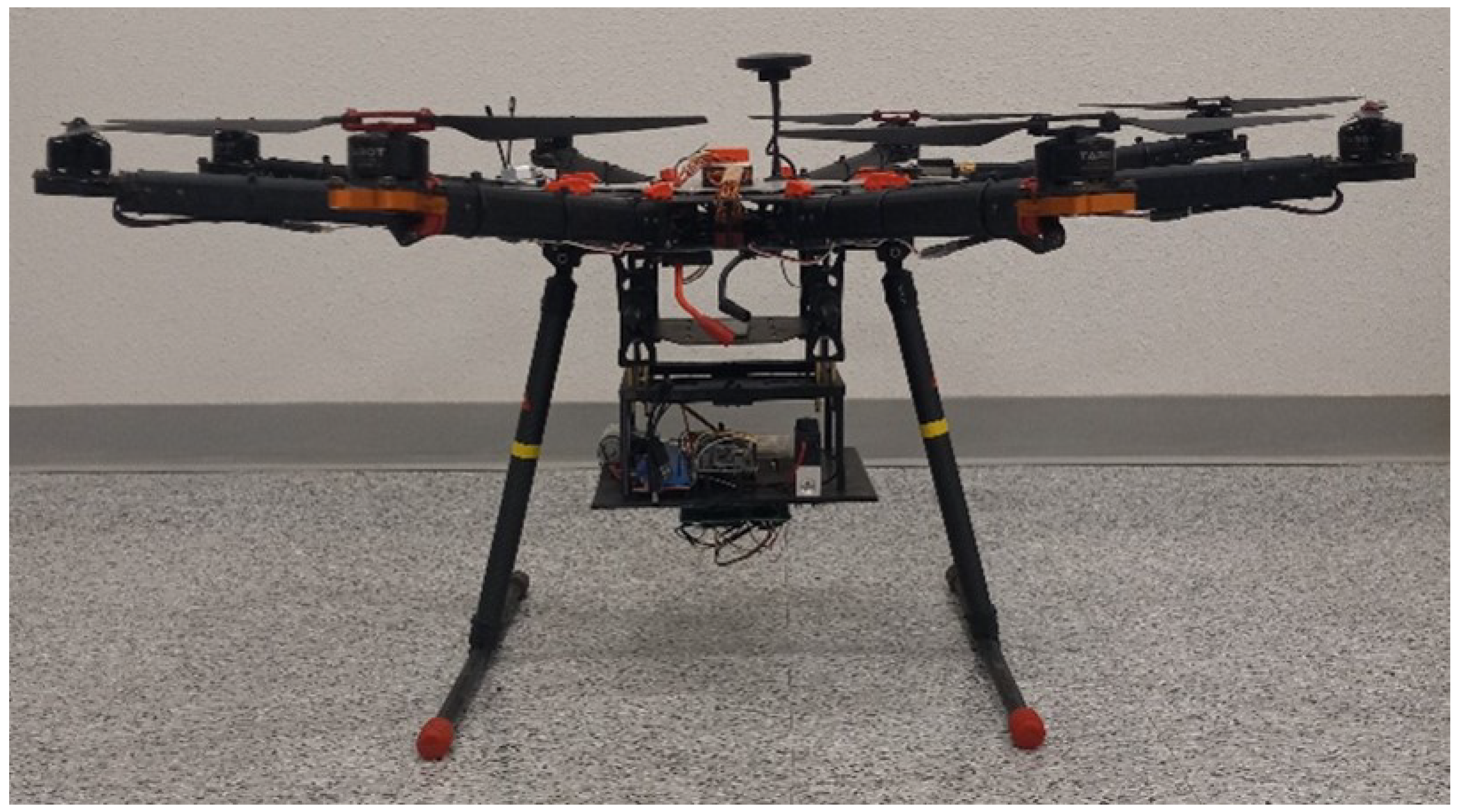
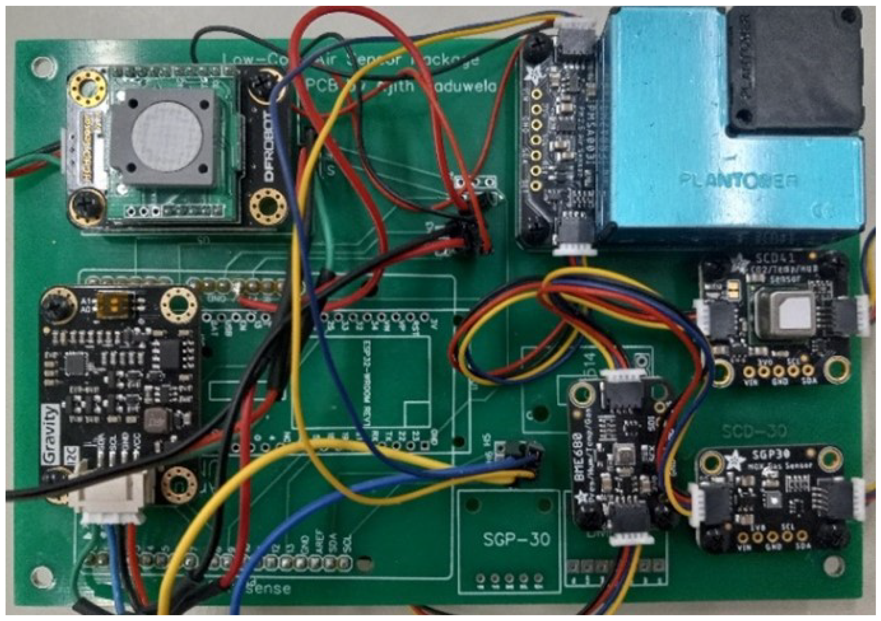
Figure 1 and Figure 2 show the UAV platform and air quality sensor package that was used to collect the chemical data necessary for learning the model. Table 1 outlines the various sensors used in our air quality sensor package and their specifications. Our previous works include technical details on the UAV platform as well as the air quality sensor package [12].
2.2. Chemical Data Collection
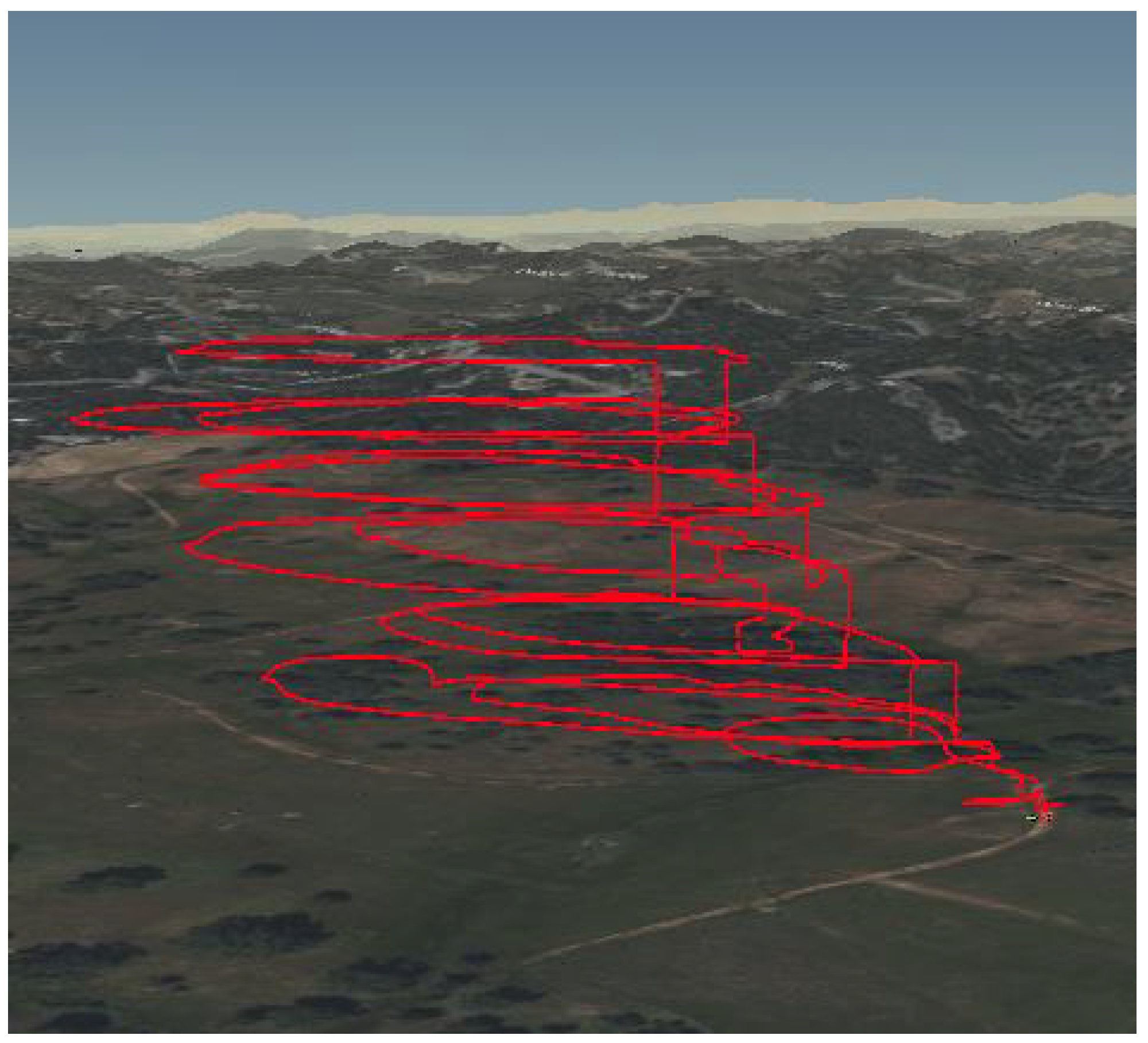
Several data collection experiments were conducted in collaboration with CAL FIRE during their prescribed burn events. The UAV was flown around and through the smoke plumes emitted by the fires. Figure 3 shows the UAV collecting data during one of these data collection experiments. We utilized data from two different experiments for learning and testing our model. The sensor package can detect a range of chemicals including CO2, CO, PM2.5 and total volatile organic compounds (VOCs). However, for the purposes of modeling plume dynamics, the chemical that was used for learning and testing our model is CO2.
In order to learn a dynamic system model for a spatiotemporal field using the method presented by [44], three possible motion strategies were outlined as follows:
- (1)
- Use one mobile sensing robot where the robot must stop at each waypoint for more than one time step to collect data at that point.
- (2)
- Use one mobile sensing robot and one static reference sensor where the mobile sensor can continuously move while collecting data and the static sensor continuously collects data at a specific location within the field being sampled. For this to work, the static sensor must be the same as the mobile sensor and both must be synchronized in time.
- (3)
- Use multiple mobile robots where all robots start at different waypoints but follow the same trajectory such that if one robot collects data at a specific waypoint at the current time step, another robot will collect measurements at that waypoint in the future time step.
The first two options were explored in this study. In each case, the UAV must collect data using a periodic trajectory. This means that measurements must be taken at the same points in space at different points in time. Figure 4 shows the trajectory executed by the UAV during the first experiment where the first motion strategy was utilized and Figure 5 shows the trajectory executed by the UAV during the second experiment where the second motion strategy was utilized. A static reference sensor that is identical to the sensor package onboard the UAV was used to collect data within the field being sampled during the second experiment. A wind sensor (YOUNG Model 91000 ResponseONE™ Ultrasonic Anemometer) was also used to measure wind speed and direction. Both sensors were mounted on a metal boom 10m high and placed 60 m downwind of the source of the smoke and along the centerline of the smoke plume. The chemical data from the air quality sensor package were synchronized with the UAV’s GPS data to produce 3D spatial plots as shown in Figure 6 and Figure 7. From the first data collection experiment, 332 data points were used to learn the model and from the second data collection experiment, 840 data points were used to learn the model.
2.3. Spatio-Temporal Modelling
A spatiotemporal field can generally be described by (1) where can represent any quantity that changes in both space and time. In our case, is the chemical concentration at a specific location within the field, denoted by q, and occurring at a specific time, denoted by t. This representation can be decomposed into the product of static spatial basis functions with time-changing weights
where and .
The spatial basis functions can take different forms such as Fourier or wavelet kernels. However, we choose the Gaussian radial basis function which is represented by
where K is a scaling coefficient, are the centers of the basis functions and is a deviation parameter.
The time-changing weights can be represented using a linear discrete stochastic state-space model which is a common representation of a dynamical system
A is a matrix that contains information on the dynamics of the spatiotemporal field. The eigenvalues of the A matrix will allow us to determine how the time-changing weights evolve over time. represents process noise.
From this model of a dynamic spatiotemporal field, the unknown parameters that must be learned from data are K, , , and A. The following subsection shows how these parameters are determined.
2.4. Learning the Spatiotemporal Model from Data
The method used for learning the A matrix is based on subspace identification [46,47,48] which is a common method for learning linear state space models. To apply this method to our specific case, we follow the steps outlined by [44].
Firstly, the data collected by the UAV must be formatted into a stacked column vector as follows
where is the chemical concentration measurement at time t, r is the number of time steps that the UAV stays at each waypoint that it stops to collect measurements and and d are user-defined parameters. Following a periodic trajectory, multiple measurements are collected at each waypoint along the trajectory as the UAV continuously returns to each waypoint. All the measurements can be stacked into a block Hankel matrix as follows
where is the time taken from one measurement to the next at the same point in space.
The time-changing weights can be stacked into the following matrix
An extended observability matrix, which contains the A matrix, can be defined as
The block Hankel matrix can also be represented as
The main idea is that the extended observability matrix as well as the time-changing weights can be learned from the block Hankel matrix using singular value decomposition
Two submatrices are then extracted from the extended observability matrix
The A matrix can then be determined from the two submatrices as follows
In the case of the second motion strategy where a static reference sensor is used, the measurements will then be stacked as follows
where represents the measurement taken by the static reference sensor at time t.
The observability matrix will then be represented by
The remaining unknown parameters K, and can be learned using nonlinear optimization as follows
2.5. Comparison with Existing Model
The predictions from our data-driven spatiotemporal model were compared to the predictions of the commonly used Gaussian puff model [49,50,51,52] which is a physics-based spatiotemporal model. The model assumes that the concentration at any point within a field is the summation of the contributions of different puffs that were emitted by a single source. Unlike the Gaussian plume model which assumes steady state conditions such as constant emission rate and wind speed, the Gaussian puff model assumes that these parameters change with time, and therefore, the concentrations at points within the field change in time. The model is described as
where is the concentration of a single puff at point at time t. Q is the emission rate from the chemical source. u is the horizontal wind speed along the centerline of the plume. and are the standard deviations of the emission distributions in the vertical and horizontal directions, respectively. is the height of the plume centerline above the ground. Since we collected chemical, GPS and wind speed data and the deviation parameters are functions of position, the only unknown parameter in this model is the emission rate Q, which we cannot measure. Therefore, we utilized the data we collected to estimate this parameter. This was achieved by using linear least squares regression which allows us to find the line of best fit that matches the GPS and chemical data collected. The estimated Q was then used in computing the Gaussian puff model. An average wind speed was used when learning Q to simplify the process and the model was then computed using the fluctuating wind speeds that were measured.
To evaluate both models, their predicted values were compared to the actual measured values. This was conducted using the mean absolute error (MAE) and the root mean squared error (RMSE) between the predicted and measured values. Both metrics are commonly used to assess the accuracy of predictive models, each providing its own advantages. MAE is more easily interpreted whereas RMSE is more sensitive to outliers in the data.
Furthermore, since a normal distribution is assumed for both models, a Chi-square goodness-of-fit test was conducted for each model. This test is commonly used to determine the likelihood that a variable comes from a specific distribution or not. The test was conducted based on a null hypothesis that the predicted values form a normal distribution with a mean and variance that was estimated from the measured data. The associated p-values for the hypothesis test were also calculated.
3. Results
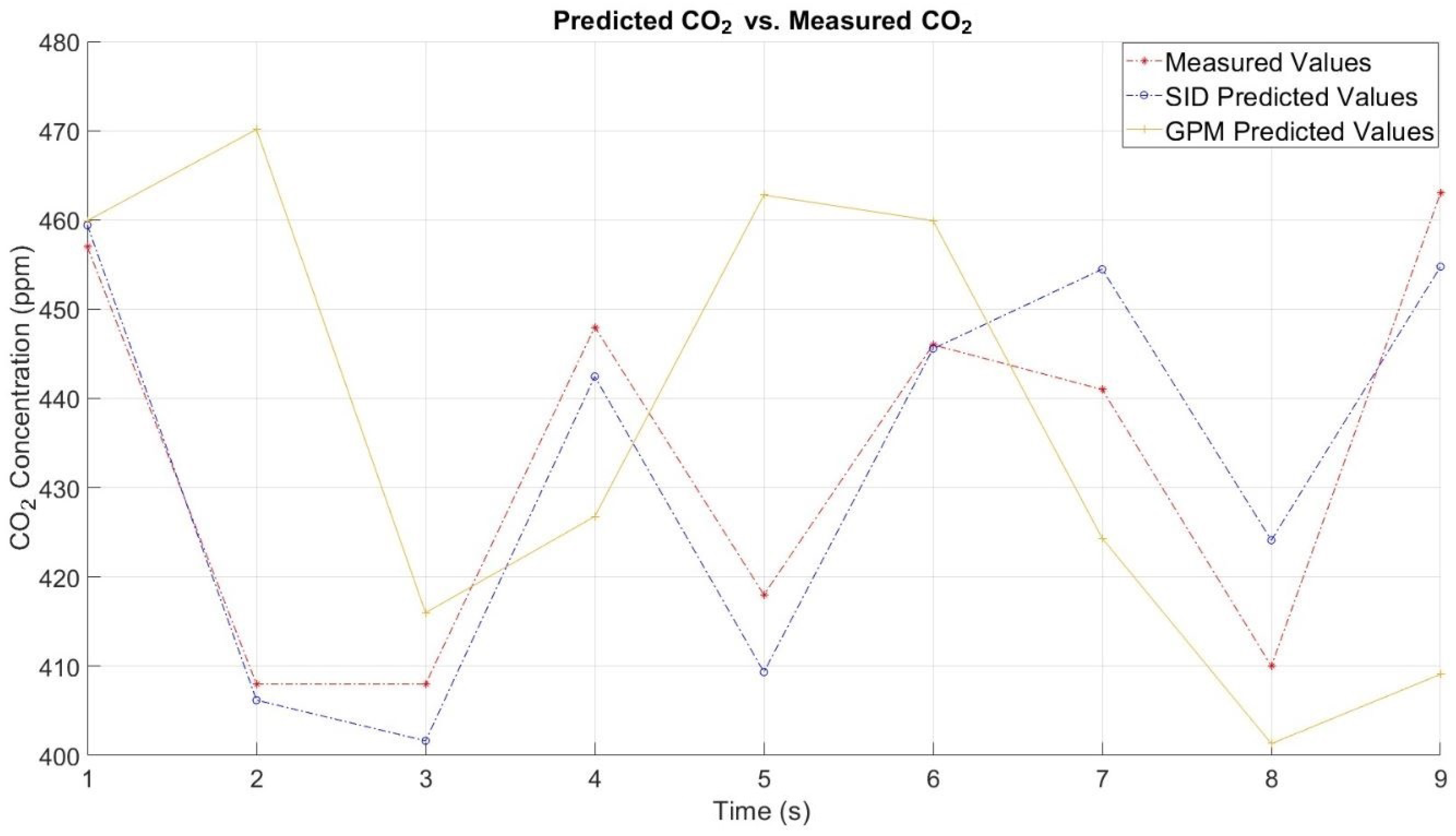
Figure 8 shows our modeling results using the data collected at the first experiment to learn the model parameters. The plot shows CO2 concentration predictions of our SID model and the GPM against the actual measured values at a random point within the field and at different points in time. In general, closer agreement between the SID model predictions and the measured values, as compared to the GPM predictions, can be observed. Specifically, for the SID model the MAE between the predicted and measured values is 6.782 ppm whereas the MAE for the GPM is 25.799 ppm. Also, the RMSE for the SID model is 8.193 ppm whereas the RMSE for the GPM is 33.068 ppm.
Figure 9 shows our modeling results using the data collected from the second experiment to learn the model parameters. Similar to the first experiment, closer agreement between the SID model predictions and the measured values, as compared to the GPM predictions, can be observed. Specifically, for the SID model, the MAE between the predicted and measured values is 30.01 ppm whereas the MAE for the GPM is 104.492 ppm. Also, the RMSE for the SID model is 47.288 ppm whereas the RMSE for the GPM is 129.493 ppm. From both experiments it can be concluded that the SID model showed consistently better performance than the GPM.
A Chi-square goodness-of-fit test was conducted for each model using MATLAB’s chi2gof function. In this test, the null hypothesis is that the predicted values form a normal distribution with a mean and variance that was estimated from the measured data. For the first experiment, the test returned a comment indicating that after pooling, some bins still have low expected counts and that the chi-square approximation may not be accurate. This is due to the lack of data from the first experiment. For the second experiment, where more data were available, the test returned Chi-square values of 15.3587 for the SID model and 12.2009 for the GPM model. The associated p-values for the SID model and the GPM are 0.0047 and 0.0321, respectively.
Figure 10 shows the predicted field from the SID model for all points within a 100 m × 100 m 2D area as they change in time. Snapshots of the field at four different time steps throughout the simulation (5, 10, 15 and 20 s) are displayed. Figure 11 shows the corresponding results at the same time steps for the GPM during the simulation.
4. Discussion
From Figure 8 and Figure 9, it can be seen that in both cases, our SID model predicts the CO2 concentration with a higher accuracy than the GPM. It should be noted that the testing of the models was conducted at random points along the UAV’s trajectory that were not used for learning the model, using the same data set. Cross-validation using an independent data set was not possible due to the limited data collected. Additionally, based on the limited measurements collected during the first experiment, we can only validate the model up to nine future predictions. However, for the second experiment, since much more data were collected, we can validate the model up to 27 future predictions. Although the GPM is a physics-based model, we used the data collected to learn the one unknown parameter, which is the emission rate Q. Therefore, the GPM was implemented in a data-driven manner. This was conducted in order to ensure that the comparison was as fair as possible. Both our model and the GPM assume a Gaussian distribution of the chemical concentrations. However, in the case of the GPM, the Gaussian distribution is along the centerline of the plume in the horizontal and vertical directions whereas for our model, the Gaussian distribution occurs in all directions (circle for 2D and sphere for 3D). Furthermore, the distribution is based on several basis centers which can be increased as the order of the model is increased. For the first experiment, the UAV conducted nine cycles of a periodic trajectory and these were enough data to learn a fifth-order model whereas for the second experiment, the UAV conducted 27 cycles of a periodic trajectory and these were enough data to learn a 10th-order model. To learn a higher-order model, however, much more data must be collected since the number of data points must be much greater than the order of the model.
From Figure 10 and Figure 11, as the time steps increase, we can observe the changes in concentrations throughout the field. The area sampled during data collection was approximately 60 m in diameter. It should be noted that since data could only be collected along the trajectory of the UAV, we do not have measurements at other locations within the field to validate the entire field prediction for either of the models. We can only validate the models at specific points in space for different points in time as shown in Figure 8 and Figure 9. However, for the entire field predictions, we can compare the performance of both models in terms of the expected behavior of a plume dynamic model. In the case of the SID model, after 20 s, the concentrations of the chemical pollutants are significant enough to be observed up to 100 m away, whereas the concentrations predicted by the GPM are only observed at 20 m away. The main reason for this is that in reality there is no single source of smoke and smoke was generated at many different locations throughout the fire perimeter. This can be clearly seen in Figure 3. However, when implementing the GPM, it is commonly assumed that the smoke is emitted from a single-point source. Another reason for the differences in predictions is that the GPM depends heavily on wind speed which is different at every time step. Our wind speed measurements were not taken onboard the UAV but were taken from the ground at a height of 10m. The wind speed measurement at the location of the UAV as it moves will of course be different. The GPM also depends heavily on assumptions of atmospheric stability which affects the calculation of the standard deviation parameters and, in turn, affects the predicted concentrations.
From the Chi-square goodness-of-fit test, the conclusion that can be drawn from this result is that both models reject the null hypothesis, and therefore, the predicted values do not come from a normal distribution. This test was conducted using limited testing data points and further testing should be conducted to properly evaluate the models using more data and by evaluating the models based on different distributions.
5. Conclusions
This study focused on developing a data-driven spatiotemporal model for predicting smoke plume dynamics in both space and time. The model is also a control-theoretic model which makes it suitable for application to model-based control techniques for smoke plume tracking. Subspace identification and nonlinear optimization methods were applied to develop the model. The results generally showed good performance of the model when the predicted values were compared to the actual measured values. Furthermore, the model generally outperformed the commonly used Gaussian puff model. The next step in this work will be to collect data using multiple UAVs in order to learn a more accurate plume dynamic model. Future work also includes applying this model to a model-based controller on a UAV to test its capabilities in tracking a wildfire smoke plume.
Author Contributions
Conceptualization, Z.K. and P.R.; methodology, X.L., A.K. and P.R.; software, X.L. and P.R.; validation, A.K. and A.W.; formal analysis, Z.K.; investigation, Z.K. and A.K.; resources, A.W. and X.L.; data curation, P.R.; writing—original draft preparation, P.R.; writing—review and editing, P.R., Z.K. and A.W.; visualization, P.R.; supervision, Z.K.; project administration, Z.K.; funding acquisition, Z.K. All authors have read and agreed to the published version of the manuscript.
Funding
This research was funded by Sony Corporation, grant number A21-3976.
Institutional Review Board Statement
Not applicable.
Informed Consent Statement
Not applicable.
Data Availability Statement
Data supporting reported results can be found at: https://github.com/CHPS-Lab/uav_wildfire (accessed on 31 January 2024).
Acknowledgments
We are grateful to David Passovoy from the California Department of Forestry and Fire Protection (CAL FIRE) for providing us with opportunities to collect data during prescribed burn events and assisting us tremendously with this data collection process. We are also grateful to Sarika Kulkarni from the California Air Resources Board (CARB) for providing us with knowledge on physics-based atmospheric dispersion models.
Conflicts of Interest
The authors declare no conflicts of interest. The funders had no role in the design of the study; in the collection, analyses, or interpretation of data; in the writing of the manuscript; or in the decision to publish the results.
Abbreviations
The following abbreviations are used in this manuscript:
| UAV | Unmanned Aerial Vehicle |
| VOC | Volatile Organic Compound |
| SID | Subspace Identification |
| GPM | Gaussian Puff Model |
| MAE | Mean Absolute Error |
| RMSE | Root Mean Squared Error |
| ppm | Parts Per Million |
| CAL FIRE | California Department of Forestry and Fire Protection |
| CARB | California Air Resources Board |
References
- Sullivan, A.L. Wildland surface fire spread modelling, 1990–2007. 2: Empirical and quasi-empirical models. Int. J. Wildland Fire 2009, 18, 369–386. [Google Scholar] [CrossRef]
- ALERTCalifornia. Available online: https://alertcalifornia.org/ (accessed on 27 March 2024).
- EOSDIS Worldview. Available online: https://worldview.earthdata.nasa.gov/ (accessed on 27 March 2024).
- Jain, P.; Coogan, S.C.; Subramanian, S.G.; Crowley, M.; Taylor, S.; Flannigan, M.D. A review of machine learning applications in wildfire science and management. Environ. Rev. 2020, 28, 478–505. [Google Scholar] [CrossRef]
- Bailon-Ruiz, R.; Lacroix, S. Wildfire remote sensing with UAVs: A review from the autonomy point of view. In Proceedings of the 2020 International Conference on Unmanned Aircraft Systems (ICUAS), Athens, Greece, 1–4 September 2020; IEEE: Piscateville, NJ, USA, 2020; pp. 412–420, ISBN 9781728142784. [Google Scholar] [CrossRef]
- Bouguettaya, A.; Zarzour, H.; Taberkit, A.M.; Kechida, A. A review on early wildfire detection from unmanned aerial vehicles using deep learning-based computer vision algorithms. Signal Process. 2022, 190, 108309. [Google Scholar] [CrossRef]
- Mohsan, S.A.H.; Khan, M.A.; Noor, F.; Ullah, I.; Alsharif, M.H. Towards the Unmanned Aerial Vehicles (UAVs): A Comprehensive Review. Drones 2022, 6, 147. [Google Scholar] [CrossRef]
- Mohsan, S.A.H.; Othman, N.Q.H.; Li, Y.; Alsharif, M.H.; Khan, M.A. Unmanned aerial vehicles (UAVs): Practical aspects, applications, open challenges, security issues, and future trends. Intell. Serv. Robot. 2023, 16, 109–137. [Google Scholar] [CrossRef]
- Zhang, Z.; Zhu, L. A Review on Unmanned Aerial Vehicle Remote Sensing: Platforms, Sensors, Data Processing Methods, and Applications. Drones 2023, 7, 398. [Google Scholar] [CrossRef]
- Burgués, J.; Marco, S. Environmental chemical sensing using small drones: A review. Sci. Total. Environ. 2020, 748, 141172. [Google Scholar] [CrossRef] [PubMed]
- Maqbool, A.; Mirza, A.; Afzal, F.; Shah, T.; Khan, W.Z.; Zikria, Y.B.; Kim, S.W. System-Level Performance Analysis of Cooperative Multiple Unmanned Aerial Vehicles for Wildfire Surveillance Using Agent-Based Modeling. Sustainability 2022, 14, 5927. [Google Scholar] [CrossRef]
- Ragbir, P.; Kaduwela, A.; Passovoy, D.; Amin, P.; Ye, S.; Wallis, C.; Alaimo, C.; Young, T.; Kong, Z. UAV-Based Wildland Fire Air Toxics Data Collection and Analysis. Sensors 2023, 23, 3561. [Google Scholar] [CrossRef]
- Reid, C.E.; Brauer, M.; Johnston, F.H.; Jerrett, M.; Balmes, J.R.; Elliott, C.T. Critical Review of Health Impacts of Wildfire Smoke Exposure. Environ. Health Perspect. 2016, 124, 1334–1343. [Google Scholar] [CrossRef] [PubMed]
- Ford, B.; Val Martin, M.; Zelasky, S.E.; Fischer, E.V.; Anenberg, S.C.; Heald, C.L.; Pierce, J.R. Future Fire Impacts on Smoke Concentrations, Visibility, and Health in the Contiguous United States. GeoHealth 2018, 2, 229–247. [Google Scholar] [CrossRef] [PubMed]
- Larsen, A.E.; Reich, B.J.; Ruminski, M.; Rappold, A.G. Impacts of fire smoke plumes on regional air quality, 2006–2013. J. Expo. Sci. Environ. Epidemiol. 2018, 28, 319–327. [Google Scholar] [CrossRef] [PubMed]
- Fann, N.; Alman, B.; Broome, R.A.; Morgan, G.G.; Johnston, F.H.; Pouliot, G.; Rappold, A.G. The health impacts and economic value of wildland fire episodes in the U.S.: 2008–2012. Sci. Total. Environ. 2018, 610–611, 802–809. [Google Scholar] [CrossRef] [PubMed]
- Cascio, W.E. Wildland fire smoke and human health. Sci. Total. Environ. 2018, 624, 586–595. [Google Scholar] [CrossRef] [PubMed]
- Liu, Y.; Heilman, W.E.; Potter, B.E.; Clements, C.B.; Jackson, W.A.; French, N.H.F.; Goodrick, S.L.; Kochanski, A.K.; Larkin, N.K.; Lahm, P.W.; et al. Smoke Plume Dynamics. In Wildland Fire Smoke in the United States: A Scientific Assessment; Peterson, D.L., McCaffrey, S.M., Patel-Weynand, T., Eds.; Springer International Publishing: Cham, Switzerland, 2022; pp. 83–119. ISBN 9783030870454. [Google Scholar] [CrossRef]
- Zannetti, P. The Tool—Mathematical Modeling. In Air Pollution Modeling: Theories, Computational Methods and Available Software; Zannetti, P., Ed.; Springer: Boston, MA, USA, 1990; pp. 27–40. ISBN 9781475744651. [Google Scholar] [CrossRef]
- Johnson, J.B. An Introduction to Atmospheric Pollutant Dispersion Modelling. In Proceedings of the ECAS, online, 14 July 2022; MDPI: Basel, Switzerland, 2022; p. 18. [Google Scholar] [CrossRef]
- Nanni, A.; Tinarelli, G.; Solisio, C.; Pozzi, C. Comparison between Puff and Lagrangian Particle Dispersion Models at a Complex and Coastal Site. Atmosphere 2022, 13, 508. [Google Scholar] [CrossRef]
- Jia, M.; Daniels, W.; Hammerling, D. Comparison of the Gaussian plume and puff atmospheric dispersion models for methane modeling on oil and gas sites. ChemRxiv, 2023; preprint. [Google Scholar] [CrossRef]
- Lee, J.; Lee, S.; Son, H.; Yi, W.H. Development of PUFF–Gaussian dispersion model for the prediction of atmospheric distribution of particle concentration. Sci. Rep. 2021, 11, 6456. [Google Scholar] [CrossRef] [PubMed]
- Cao, X.; Roy, G.; Hurley, W.J.; Andrews, W.S. Dispersion Coefficients for Gaussian Puff Models. Bound.-Layer Meteorol. 2011, 139, 487–500. [Google Scholar] [CrossRef]
- Mandel, J.; Beezley, J.D.; Kochanski, A.K. Coupled atmosphere-wildland fire modeling with WRF-Fire. Geosci. Model Dev. Discuss. 2011, 4, 497–545. [Google Scholar] [CrossRef]
- Yanosky, J.D.; Paciorek, C.J.; Laden, F.; Hart, J.E.; Puett, R.C.; Liao, D.; Suh, H.H. Spatio-temporal modeling of particulate air pollution in the conterminous United States using geographic and meteorological predictors. Environ. Health 2014, 13, 63. [Google Scholar] [CrossRef]
- Dimakopoulou, K.; Samoli, E.; Analitis, A.; Schwartz, J.; Beevers, S.; Kitwiroon, N.; Beddows, A.; Barratt, B.; Rodopoulou, S.; Zafeiratou, S.; et al. Development and Evaluation of Spatio-Temporal Air Pollution Exposure Models and Their Combinations in the Greater London Area, UK. Int. J. Environ. Res. Public Health 2022, 19, 5401. [Google Scholar] [CrossRef]
- Iyer, S.R.; Balashankar, A.; Aeberhard, W.H.; Bhattacharyya, S.; Rusconi, G.; Jose, L.; Soans, N.; Sudarshan, A.; Pande, R.; Subramanian, L. Modeling fine-grained spatio-temporal pollution maps with low-cost sensors. Npj Clim. Atmos. Sci. 2022, 5, 76. [Google Scholar] [CrossRef]
- Sampson, P.D.; Szpiro, A.A.; Sheppard, L.; Lindström, J.; Kaufman, J.D. Pragmatic estimation of a spatio-temporal air quality model with irregular monitoring data. Atmos. Environ. 2011, 45, 6593–6606. [Google Scholar] [CrossRef]
- Sánchez-Balseca, J.; Pérez-Foguet, A. Spatio-temporal air pollution modelling using a compositional approach. Heliyon 2020, 6, e04794. [Google Scholar] [CrossRef]
- Le, V.D. Spatiotemporal Graph Convolutional Recurrent Neural Network Model for Citywide Air Pollution Forecasting. arXiv 2023, arXiv:2304.12630. [Google Scholar] [CrossRef]
- Beloconi, A.; Probst-Hensch, N.M.; Vounatsou, P. Spatio-temporal modelling of changes in air pollution exposure associated to the COVID-19 lockdown measures across Europe. Sci. Total. Environ. 2021, 787, 147607. [Google Scholar] [CrossRef]
- Tsokov, S.; Lazarova, M.; Aleksieva-Petrova, A. A Hybrid Spatiotemporal Deep Model Based on CNN and LSTM for Air Pollution Prediction. Sustainability 2022, 14, 5104. [Google Scholar] [CrossRef]
- Amato, F.; Guignard, F.; Robert, S.; Kanevski, M. A novel framework for spatio-temporal prediction of environmental data using deep learning. Sci. Rep. 2020, 10, 22243. [Google Scholar] [CrossRef]
- Zhang, K.; Zhang, X.; Song, H.; Pan, H.; Wang, B. Air Quality Prediction Model Based on Spatiotemporal Data Analysis and Metalearning. Wirel. Commun. Mob. Comput. 2021, 2021, 9627776. [Google Scholar] [CrossRef]
- Alyousifi, Y.; Ibrahim, K.; Kang, W.; Zin, W.Z.W. Modeling the spatio-temporal dynamics of air pollution index based on spatial Markov chain model. Environ. Monit. Assess. 2020, 192, 719. [Google Scholar] [CrossRef] [PubMed]
- Peralta, B.; Sepúlveda, T.; Nicolis, O.; Caro, L. Space-Time Prediction of PM2.5 Concentrations in Santiago de Chile Using LSTM Networks. Appl. Sci. 2022, 12, 11317. [Google Scholar] [CrossRef]
- Liu, H.; Han, Q.; Sun, H.; Sheng, J.; Yang, Z. Spatiotemporal adaptive attention graph convolution network for city-level air quality prediction. Sci. Rep. 2023, 13, 13335. [Google Scholar] [CrossRef]
- Zhang, J.; Zhao, X. Three-dimensional spatiotemporal wind field reconstruction based on physics-informed deep learning. Appl. Energy 2021, 300, 117390. [Google Scholar] [CrossRef]
- Muthukumar, P.; Nagrecha, K.; Comer, D.; Calvert, C.F.; Amini, N.; Holm, J.; Pourhomayoun, M. PM2.5 Air Pollution Prediction through Deep Learning Using Multisource Meteorological, Wildfire, and Heat Data. Atmosphere 2022, 13, 822. [Google Scholar] [CrossRef]
- Jadaliha, M.; Lee, J.; Choi, J. Adaptive Control of Multiagent Systems for Finding Peaks of Uncertain Static Fields. J. Dyn. Syst. Meas. Control. 2012, 134, 051007. [Google Scholar] [CrossRef]
- Salam, T.; Hsieh, M.A. Adaptive Sampling and Reduced-Order Modeling of Dynamic Processes by Robot Teams. IEEE Robot. Autom. Lett. 2019, 4, 477–484. [Google Scholar] [CrossRef]
- Leonard, N.E.; Paley, D.A.; Lekien, F.; Sepulchre, R.; Fratantoni, D.M.; Davis, R.E. Collective Motion, Sensor Networks, and Ocean Sampling. Proc. IEEE 2007, 95, 48–74. [Google Scholar] [CrossRef]
- Lan, X. Learning and Monitoring of Spatio-Temporal Fields with Sensing Robots. Doctoral Dissertation, Boston University, Boston, MA, USA, 2015. Available online: https://open.bu.edu/handle/2144/13640 (accessed on 27 March 2024).
- Lan, X.; Schwager, M. Learning a dynamical system model for a spatiotemporal field using a mobile sensing robot. In Proceedings of the 2017 American Control Conference (ACC), Seattle, WA, USA, 24–26 May 2017; IEEE: Piscateville, NJ, USA, 2017; pp. 170–175, ISBN 9781509059928. [Google Scholar] [CrossRef]
- Van Overschee, P.; De Moor, B. Subspace Identification for Linear Systems; Springer: Boston, MA, USA, 1996; ISBN 9781461380610/9781461304654. [Google Scholar] [CrossRef]
- Katayama, T. Subspace Methods for System Identification; Springer: London, UK, 2005; ISBN 9781852339814/9781846281587. [Google Scholar] [CrossRef]
- Qin, S.J. An overview of subspace identification. Comput. Chem. Eng. 2006, 30, 1502–1513. [Google Scholar] [CrossRef]
- Ermak, D.L. An analytical model for air pollutant transport and deposition from a point source. Atmos. Environ. (1967) 1977, 11, 231–237. [Google Scholar] [CrossRef]
- Fisher, B.E.A.; Macqueen, J.F. A Theoretical Model for Particulate Transport from an Elevated Source in the Atmosphere. IMA J. Appl. Math. 1981, 27, 359–371. [Google Scholar] [CrossRef]
- Llewelyn, R.P. An analytical model for the transport, dispersion and elimination of air pollutants emitted from a point source. Atmos. Environ. (1967) 1983, 17, 249–256. [Google Scholar] [CrossRef]
- Okamoto, S.; Ohnishi, H.; Yamada, T.; Mikami, T.; Momose, S.; Shinji, H.; Itohiya, T. A model for simulating atmospheric dispersion in low-wind conditions. Int. J. Environ. Pollut. 2001, 16, 69. [Google Scholar] [CrossRef]
Figure 1.
Octocopter unmanned aerial vehicle equipped with air quality sensor packaged for chemical data collection.
Figure 1.
Octocopter unmanned aerial vehicle equipped with air quality sensor packaged for chemical data collection.

Figure 2.
Air quality sensor package with six low-cost real-time sensors for chemical data collection.
Figure 2.
Air quality sensor package with six low-cost real-time sensors for chemical data collection.

Figure 3.
Chemical data collection during prescribed burn using the UAV equipped with the air quality sensor package.
Figure 3.
Chemical data collection during prescribed burn using the UAV equipped with the air quality sensor package.

Figure 4.
Periodic trajectory executed by UAV during data collection in first experiment.

Figure 5.
Periodic trajectory executed by UAV during data collection in second experiment.

Figure 6.
3D spatial distribution of CO2 from data collected in first experiment.

Figure 7.
3D spatial distribution of CO2 from data collected in second experiment.

Figure 8.
Predicted values for both models vs. the measured values for the first experiment.

Figure 9.
Predicted values for both models vs. the measured values for the second experiment.

Figure 10.
Subspace identification model 2D field predictions of CO2 concentration at timesteps of (a) 5 s, (b) 10 s, (c) 15 s and (d) 20 s. The x-axis and y-axis represent longitude and latitude, respectively.
Figure 10.
Subspace identification model 2D field predictions of CO2 concentration at timesteps of (a) 5 s, (b) 10 s, (c) 15 s and (d) 20 s. The x-axis and y-axis represent longitude and latitude, respectively.

Figure 11.
Gaussian puff model 2D field predictions of CO2 concentration at timesteps of (a) 5 s, (b) 10 s, (c) 15 s and (d) 20 s. The x-axis and y-axis represent longitude and latitude, respectively.
Figure 11.
Gaussian puff model 2D field predictions of CO2 concentration at timesteps of (a) 5 s, (b) 10 s, (c) 15 s and (d) 20 s. The x-axis and y-axis represent longitude and latitude, respectively.


Table 1.
Air quality sensors used for the sensor package and their specifications.
| Sensor | Measurement | Operating Range |
|---|---|---|
| Temperature | −40 to 85 °C | |
| BME680 | Barometric Pressure | 300 to 1100 hPa |
| Relative Humidity | 0 to 100% r.H. | |
| SGP30 | eCO2 | 400–60,000 ppm |
| Total VOC | 0–60,000 ppb | |
| SCD41 | CO2 | 400–5000 ppm |
| PMSA003I | Particulate Matter | 0–500 g/m3 |
| SEN0231 | Formaldehyde (HCHO) | 0–5 ppm |
| CO | 1–1000 ppm | |
| MiCS-4514 | NO2 | 0.05–10 ppm |
| NH3 | 1–500 ppm |
Disclaimer/Publisher’s Note: The statements, opinions and data contained in all publications are solely those of the individual author(s) and contributor(s) and not of MDPI and/or the editor(s). MDPI and/or the editor(s) disclaim responsibility for any injury to people or property resulting from any ideas, methods, instructions or products referred to in the content. |
© 2024 by the authors. Licensee MDPI, Basel, Switzerland. This article is an open access article distributed under the terms and conditions of the Creative Commons Attribution (CC BY) license (https://creativecommons.org/licenses/by/4.0/).
Share and Cite
MDPI and ACS Style
Ragbir, P.; Kaduwela, A.; Lan, X.; Watts, A.; Kong, Z. A Control-Theoretic Spatio-Temporal Model for Wildfire Smoke Propagation Using UAV-Based Air Pollutant Measurements. Drones 2024, 8, 169. https://doi.org/10.3390/drones8050169
AMA Style
Ragbir P, Kaduwela A, Lan X, Watts A, Kong Z. A Control-Theoretic Spatio-Temporal Model for Wildfire Smoke Propagation Using UAV-Based Air Pollutant Measurements. Drones. 2024; 8(5):169. https://doi.org/10.3390/drones8050169
Chicago/Turabian StyleRagbir, Prabhash, Ajith Kaduwela, Xiaodong Lan, Adam Watts, and Zhaodan Kong. 2024. "A Control-Theoretic Spatio-Temporal Model for Wildfire Smoke Propagation Using UAV-Based Air Pollutant Measurements" Drones 8, no. 5: 169. https://doi.org/10.3390/drones8050169