The Thermal Conductivity of Periodic Particulate Composites as Obtained from a Crystallographic Mode of Filler Packing

Abstract

In this paper, an icosahedral non-body-centered model is presented to simulate the periodic structure of a general class of homogeneous particulate composites, by predicting the particle arrangement. This model yielded three different variations, which correspond to three different deterministic particle configurations. In addition, the concept of a boundary interphase between matrix and inclusions was taken into account. In this framework, the influence of particle vicinity on the thermomechanical properties of the overall material was examined in parallel with the concept of boundary interphase. The simultaneous consideration of these two basic influential factors constitutes the novelty of this work. Next, by the use of this advanced model, the authors derived a closed-form expression to estimate the thermal conductivity of this type of composite. To test the validity of the model, the theoretical predictions arising from the proposed formula were compared with experimental data found in the literature, together with theoretical results obtained from several accurate formulae derived from other workers, and an adequate accordance was observed.

1. Introduction

It is known that thermal conductivity constitutes a fundamental property of solids, and the attainment of its theoretical predictions—especially for composites (periodic or not)—is a very difficult task, as the thermal conducting mechanism mainly depends on their microstructure [1]. On the other hand, the prediction of the thermomechanical properties of composite materials (fibrous or particulate) is evidently a very interesting topic, given that their properties depend on several parameters (e.g., the individual constituent properties, the filler size and volume concentration, the adhesion efficiency between inclusions and matrix, the filler distribution and possible vicinity, etc.). In this framework, Hashin and Hashin et al. [2,3] assumed that a particulate composite material is a collection of small-volume elements of various sizes and shapes which densely fill the composite. Thus, the particulates were assumed to be conglomerations of spherical inclusions and shells, with the properties of the matrix, surrounding the inclusions. In each volume element, the content of the inclusion was equal to the total content of the dispersed phase in the composite. In addition, Sideridis et al. [4] examined the effect of the adhesion between particles and matrix to determine the thermal expansion coefficient by a theoretical analysis using a modified model that includes a third phase between filler and matrix (the interphase) which has different thermomechanical properties from those of the main phases. Meanwhile, Maxwell [5] provided a general basis for estimating the effective thermal conductivity of particulate composites, whereas in References [6,7,8] some remarkable theoretical and empirical approaches were presented to analyze the thermal conductivity of composites.

Further, Bruggeman [9] generated another considerable model to calculate the thermal conductivity of composites consisting of spherical particles embedded in a continuum matrix. Here, the particle interaction was not taken into account. Nonetheless, this model is based on different assumptions regarding permeability and field strength when compared with the Maxwell model [5]. Further, one may refer to Lewis–Nielsen empirical model [10], which generally yields satisfactory results although the interfacial thermal resistance is not taken into consideration. In addition, in Reference [11] the thermal conductivity of epoxy particulate composites reinforced with aluminum particles was experimentally obtained at low and medium values of filler volume fraction.

Moreover, in Reference [12], three models of the effective thermal conductivity of concentrated particulate composites were developed via the differential effective medium approach. The first one expresses the relative thermal conductivity of a particulate composite in terms of the thermal conductivity ratio (i.e., ratio of dispersed-phase to continuous-phase conductivities) and the filler content. The other two models define this property as a function of the above two variables along with the maximum packing volume fraction of particles. Additionally, in Reference [13], the particle contiguity was taken into account to estimate the thermal expansion coefficient for pore-free homogeneous composite materials of particulate structure whilst Roudini et al. [14] also examined the influence of reinforcement contiguity on the thermal expansion of composites reinforced with alumina particles. In addition, for a detailed investigation of the thermal conductivity and diffusivity of multi-scale concrete composites by means of an effective medium theory, one may refer to Garboczi et al. [15], whereas in Reference [16] a considerable work to study the effect of an inhomogeneous interphase zone on the bulk modulus and conductivity of particulate composites containing spherical inclusions was performed. Moreover, in Reference [17] the thermal conductivity of periodic particulate composites was evaluated by a body-centered cubic model transformed into a hexaphase spherical model. This model took into account the influence of internal and neighboring particles, but neglected the interphase concept.

Concurrently, the effective thermal conductivity of a composite sphere in a continuum medium with conduct resistance was studied in Reference [18], whereas in Reference [19] thermal resistance-based bounds for the effective conductivity of composites were determined. Additionally, Agari and Uno [20] and Agari et al. [21] proposed a practical and useful approach to calculate the thermal conductivity of particulate composites, whilst Khan and Muliana [22] proposed a microstructural model to evaluate thermal conductivity and thermal expansion coefficient for particulate composites, taking into account the particle interaction.

On the other hand, in Reference [23] an advanced micromechanical model based on rigorous domain discretization techniques motivated by Voronoi polygons was developed to simulate the structure of unidirectional fibrous composites undergoing interfacial debonding. Here, it should be noticed that the computational efficiency gained by this prominent model is significant when compared with previous ones on this type of composites. Besides, in Reference [24] the thermal conductivity of homogeneous particulate composites of periodic microstructure was estimated by means of a non-body-centered model which yielded three variations: simple cubic model, side-centered cubic model, and face-centered cubic model. This model considered the particle distribution and contiguity together with the concept of interphase. Further, in Reference [25] a more advanced polyhedral model was introduced to simulate the particle arrangement of periodic particulate composites and then to evaluate their thermal conductivity.

Moreover, in Reference [26] the thermal conductivity of a general class of advanced epoxy particulate composites containing combustion-synthesized h-BN (hexagonal Boron Nitride) particles in a uniform distribution inside the matrix was evaluated.

Further, in Reference [27] Al₂O₃/epoxy composites with very high flexural strength and thermal conductivity were manufactured using a new processing technique consisting of the gelcasting, sintering, and vacuum infiltration methods. For a detailed study of thermal conductivity in composites, one may refer to a comprehensive review paper by Burger at al. [28]. Finally, an experimental work concerning the influence of filler loading, shape, arrangement, and temperature on the thermal conductivity of polymer nanocomposites was performed in Reference [29].

In the present work, the authors examine a periodic particulate composite in the frame of an icosahedral non-body-centered model yielding three different variations. In addition, the inclusions, assumed to be perfectly spherical in shape, are encircled by inhomogeneous interphase zones, the volume fractions of which are generally determined by heat capacity measurements. Next, the corresponding unit cells arising from these distinct three variations of this polyhedral model are transformed in a unified manner into a nine-phase spherical unit cell. This topological transformation is based on the equality of volume fractions between the corresponding phases of the polyhedral and its equivalent coaxial spherical unit cell, respectively. In this context, by means of this advanced multiphase model, the contiguity amongst the particles, in the form of three deterministic configurations, is examined in parallel with the boundary interphase concept, to estimate the thermal conductivity of the overall material by a modified form of Agari and Uno’s formula [20]. Indeed, it can be said that the proposed amended expression constitutes a rather improved version of the initial formula, since the related theoretical predictions for the thermal conductivity of the particulate composite show a non-negligible difference.

2. Simulation of Particle Arrangement

The majority of microstructural models aim at reproducing in space the basic cell or representative volume element (RVE) of a periodic composite (fibrous or particulate) at a microscopic scale in order to obtain a solution. Such models are usually based on the following assumptions:

(1)

A regular geometric form is generally adopted for the inclusions (usually a sphere).

(2)

Regular geometry and topology are applied for such simulations. Models can be planar or spatial. It is obvious that a three-dimensional structure is synonymous to the overall material periodic microstructure.

Now, the first variation of the proposed icosahedral model of edge L appearing in Figure 1 constitutes a three-dimensional system capable of simulating real particulate composites.

By focusing on this model, it can be observed that 30 inclusions occupy the midpoints of all edges, whereas 12 inclusions occupy the vertices of this regular polyhedron.

It is known from Euclidean geometry that the radii of the unique circumscribed and inscribed sphere respectively are given as

$$R_{20}=\frac{L}{2}\sqrt{\frac{5+\sqrt{5}}{2}}$$

(1)

$$r_{20}=L\sqrt{3}\cdot \frac{\left(3+\sqrt{5}\right)}{12}$$

(2)

and therefore

$$r_{20}=R_{20}\cdot \sqrt{\frac{5+2\sqrt{5}}{15}}$$

(3)

Moreover, since a regular icosahedron consists of 20 equilateral triangles that are obviously equal to each other, the surface area is given as

$$A_{20}=20\frac{L^2\sqrt{3}}{4}=5\sqrt{3}{L}^2$$

(4)

or equivalently

$$A_{20}=\left(10\sqrt{3}-2\sqrt{15}\right)R_{20}^2$$

(5)

The volume is given as

$$V_{20}=\frac{1}{3}{A}_{20}\cdot r_{20}=\frac{5\left(3+\sqrt{5}\right)}{12}{L}^3$$

(6)

or equivalently

$$V_{20}=\frac{2\sqrt{10+2\sqrt{5})}}{3}{R}^3$$

(7)

Next, the unit cell or RVE which corresponds uniquely to the above model can be defined as a regular icosahedron of edge 2L, which surrounds the model of Figure 1 having the same centroid and is reproduced symmetrically in space to describe a periodic particulate composite.

Then, to facilitate the mathematical analysis, utilizing the evident structural symmetries, one can transform this aforementioned unit cell into a five-phase spherical model consisting of five concentric spheres of radii a, b, c, d, and e, respectively, such that a < b < c < d < e.

The cross-sectional area of this model is illustrated in Figure 2.

The structure of this multiphase unit cell, which does not contain any interphase zone, is described as follows.

The first, third, and fifth phases (the spherical region of inner radius a and outer radius b, the sector of inner radius b and outer radius c, and the zone of inner radius d and outer radius e) represent the matrix.

In addition, the second and fourth layer represent the filler. In the meanwhile, the volume of the above-mentioned RVE (i.e., the circumscribed icosahedron of edge 2L) is given as

$$V_{\mathrm{RVE}} = \frac{5\left(3+\sqrt{5}\right)}{12}\cdot {\left(2L\right)}^3$$

(8)

Next, by assuming equal inclusions (which is not necessarily the case in reality), the volume fraction, U_f, of the fillers in the continuous matrix is given in terms of the filler radius as follows:

$$U_f =\frac{42\frac{4}{3}\pi \cdot r_f{}^3}{\frac{5\left(3+\sqrt{5}\right)}{12}\cdot {\left(2L\right)}^3}$$

(9)

with r_f denoting the filler radius, which is obviously considered as known.

The above relationship can be solved for L to yield

$$L=\sqrt[3]{\frac{84\pi \cdot r_f{}^3}{5\left(3+\sqrt{5}\right)U_f }}$$

(10)

According to the proposed topological transformation, the volume of the icosahedral unit cell of edge 2L reduces to the volume of a sphere of outer radius e. Hence, one infers

$${\left(2L\right)}^3=\frac{4}{3}\pi e^3$$

(11)

Equation (11) can be combined with Equations (9) and (10) to yield

$$e=r_f\sqrt[3]{\frac{42}{U_f}}$$

(12)

Now, let us denote as w₂₀ the midradius of the icosahedral model of Figure 1 (i.e., the distance from the centroid to the midpoint of an arbitrary edge).

From Euclidean geometry, it is known that

$$w_{20}=\frac{1}{4}\left(1+\sqrt{5}\right)L$$

(13)

Here, we may assume without violating the rigor of our mathematical formalism that the spherical sectors in the multiphase cell of Figure 2 expressing the two groups of particles in Figure 1 (i.e., 30 and 12) are equidistantly distributed on both sides of the spherical surfaces defined by radii w₂₀ and R₂₀.

Hence, these phases are developed in such a way as to be in accordance with the following equalities:

$$\begin{gathered} b^3-a^3={30r}_f^3 \\ {b}^3+a^3={2w}_{20}^3 \end{gathered}$$

(14)

and

$$\begin{gathered} d^3-c^3=12r_f^3 \\ {d}^3+c^3={2R}_{20}^3 \end{gathered}$$

(15)

The solution of the above groups of equations yields the values of a, b, c, and d in terms of filler radius as follows:

$$a=\sqrt[3]{w_{20}^3-{15r}_f^3}$$

(16)

$$b=\sqrt[3]{w_{20}^3+{15r}_f^3}$$

(17)

$$c=\sqrt[3]{R_{20}^3-{6r}_f^3}$$

(18)

$$d=\sqrt[3]{R_{20}^3+{6r}_f^3}$$

(19)

Moreover, according to some restrictions obtained from Figure 1 and concern the particle contiguity (see Appendix A for a thorough presentation), the first variation of the proposed icosahedral model is valid for filler contents at most equal to 0.15874.

Then, let us consider the second variation of the introduced non-body-centered icosahedral model (Figure 3).

By centering on this model, one can see that 20 inclusions occupy the centroids of all faces, whereas 12 inclusions occupy the vertices of this platonic solid. Following the same reasoning as before, the RVE which corresponds uniquely to the above model can be defined as a regular icosahedron of edge 2L, which surrounds the model of Figure 3 having the same centroid and is reproduced symmetrically in space to describe the material. Next, one may point out that this unit cell, after the same topological transformation that we previously carried out, results in the same five-phase spherical model of Figure 2.

The volume of the above-mentioned RVE (i.e., the concentric icosahedron of edge 2L) is given as

$$V_{\mathrm{RVE}} = \frac{5\left(3+\sqrt{5}\right)}{12}\cdot {\left(2L\right)}^3$$

(20)

Next, by assuming equal inclusions (which is not necessarily the case in reality), the volume fraction U_f of the fillers inside the continuous matrix is given in terms of the filler radius as follows:

$$U_f =\frac{42\frac{4}{3}\pi \cdot r_f{}^3}{\frac{5\left(3+\sqrt{5}\right)}{12}\cdot {\left(2L\right)}^3}$$

(21)

where r_f denotes the filler radius, which is obviously considered as known. The above relationship can be solved for L to yield

$$L=\sqrt[3]{\frac{84\pi \cdot r_f{}^3}{5\left(3+\sqrt{5}\right)U_f }}$$

(22)

Taking into account the proposed geometric transformation, the volume of a regular polyhedron of edge 2L reduces again to the volume of a sphere of radius e. Hence, from the equality between the volumes of polyhedral and spherical unit cell one infers

$${(2L)}^3=\frac{4}{3}{\pi \mathrm{e}}^3\Rightarrow e=2L\sqrt{\frac{1}{\pi }}$$

(23)

Equation (23) can be combined with (22) to yield

$$e=r_f\sqrt[3]{\frac{32}{U_f}}$$

(24)

In addition, it is obvious that the first phase of the spherical model (Figure 3) should surround the centroid axis of the regular polyhedron, and therefore the validity of Equations (14) and (15) are also extended to the second prismatic model.

Moreover, since we have already considered that in the four-phase model occurring in Figure 3 the circle of radius w₂₀ lies in the middle of the circular section denoting the third phase, Equation (13) still holds.

Hence, in proportion with the first variation, one may write out

$$b^3-a^3={20r}_f^3$$

(25)

$$b^3+a^3={2w}_{20}^3$$

(26)

$$d^3-c^3=12r_f^3$$

(27)

$$d^3+c^3={2R}_{20}^3$$

(28)

Thus, one infers

$$a=\sqrt[3]{w_{20}^3-{10r}_f^3}$$

(29)

$$b=\sqrt[3]{w_{20}^3+{10r}_f^3}$$

(30)

$$c=\sqrt[3]{R_{20}^3-{6r}_f^3}$$

(31)

$$d=\sqrt[3]{R_{20}^3+{6r}_f^3}$$

(32)

Moreover, according to some constraints obtained from Figure 3 (see Appendix A for a thorough presentation), the second variation of the proposed icosahedral model is valid for filler contents at most equal to 0.7499.

Finally, let us present the third variation of the icosahedral model (Figure 4).

Here, one may pinpoint that 20 inclusions occupy the centroids of all faces whereas 30 inclusions occupy the midpoints of the edges. By proceeding as previously, one may write out

$$U_f =\frac{50\frac{4}{3}\pi \cdot r_f{}^3}{\frac{5\left(3+\sqrt{5}\right)}{12}\cdot {\left(2L\right)}^3}$$

(33)

and therefore

$$L^3=\frac{20\pi \cdot r_f{}^3}{\left(3+\sqrt{5}\right)U_f}$$

(34)

Hence, from the equality of volumes between icosahedral and spherical unit cell it follows that

$${(2L)}^3=\frac{4}{3}{\pi \mathrm{e}}^3\Rightarrow e=r_f\sqrt[3]{\frac{50\pi }{U_f}}$$

(35)

$$b^3-a^3={20r}_f^3$$

(36)

$$b^3-a^3={2w}_{20}^3$$

(37)

$$d^3-c^3=30r_f^3$$

(38)

$$d^3-c^3=2R_{20}^3$$

(39)

and therefore

$$a=\sqrt[3]{w_{20}^3-{10r}_f^3}$$

(40)

$$b=\sqrt[3]{w_{20}^3+{10r}_f^3}$$

(41)

$$c=\sqrt[3]{R_{20}^3-{15r}_f^3}$$

(42)

$$d=\sqrt[3]{R_{20}^3+15r_f^3}$$

(43)

Finally, according to some restrictions obtained from Figure 4 (see Appendix A for a thorough presentation), the third variation of the proposed icosahedral model is valid for filler contents U_f < 0.04696, and thus one may deduce that this variation is rather impractical.

3. The Concept of Interphase—Towards a Nine-Phase Spherical model

As we mentioned before initiating our previous analysis, we are going to simulate the periodic microstructure of a homogeneous particulate composite material by means of unit cells based on icosahedral non-body centered models, when the spherical inclusions are also encircled by an inhomogeneous interphase region.

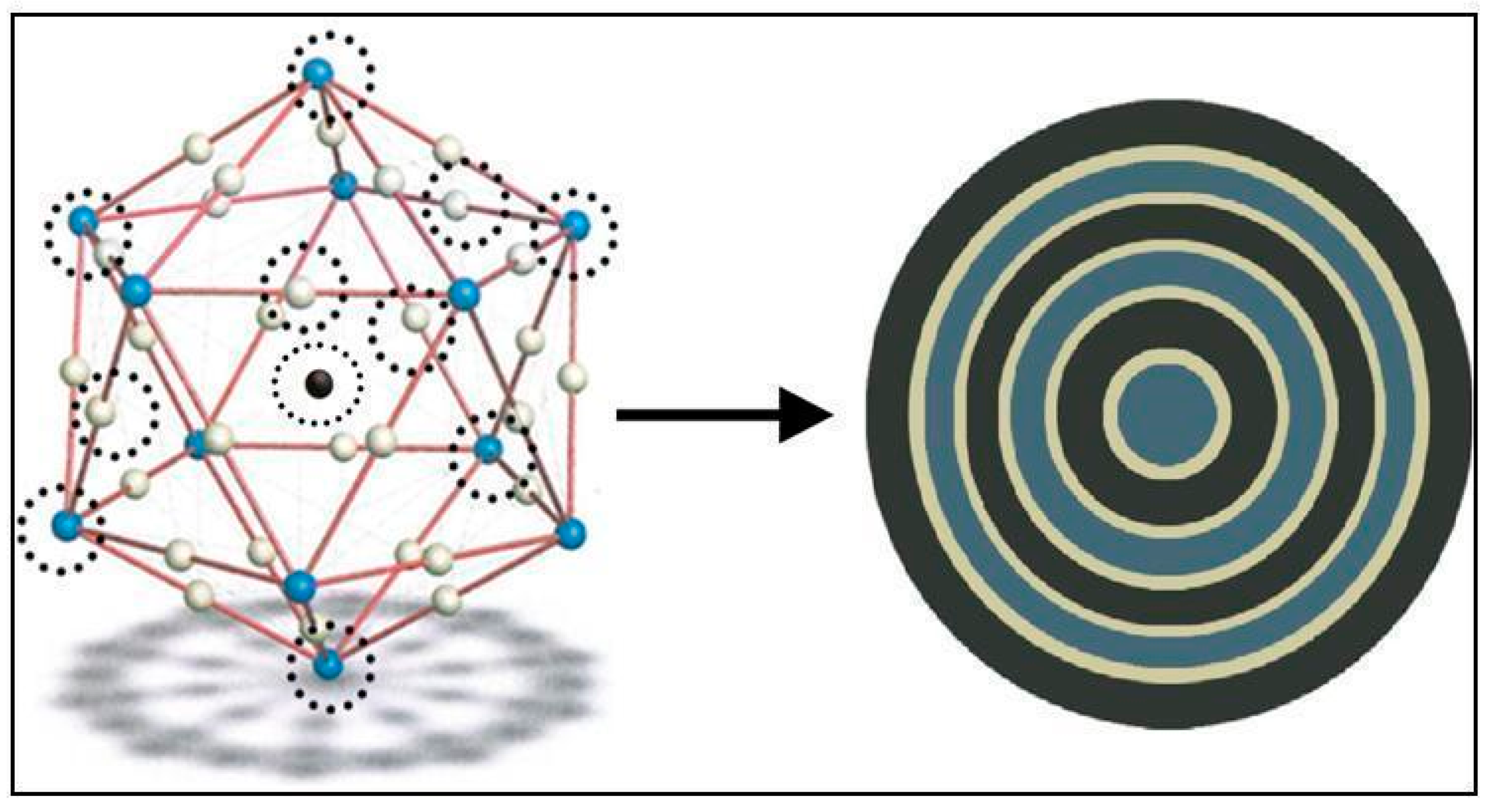
In this context, in order to perform a more refined analysis, according to the same reasoning as before, the three basic icosahedral non-body-centered models presented in Figure 1, Figure 3 and Figure 4, which are now surrounded by an inhomogeneous interphase zone of variable thermomechanical properties and are transformed into a nine-phase spherical model.

For simplicity, the unified topological transformation of the three final icosahedral unit cells into a nine-phase spherical unit cell is schematically performed in Figure 5.

Again, this topological transformation is based on the equality of volume fractions between the corresponding phases between icosahedral unit cell and its equivalent spherical one, respectively. In addition, the dotted lines around each spherical particle of the three possible non-body icosahedral variations denote the boundary interphase annuli that encircle each individual spherical inclusion. In some particles, we did not put these dotted lines in order to avoid making the shapes more complicated.

In addition, these boundary interphase zones, which are developed around each inclusion, are inhomogeneous with properties varying from that of the matrix to that of the filler, or vice versa.

The volume fraction of each interphase zone is generally determined by heat capacity measurements, as will be mentioned below.

Evidently, the following relationships hold:

$$U_f=U_3+U_7$$

(44)

$$U_i=U_2+U_4+U_6+U_8$$

(45)

$$U_m=U_1+U_5+U_9$$

(46)

Besides, since the interphase is considered somewhat as an altered matrix and its proportion is constant as developed in the interfaces of the two basic constituents of the composite, one may suppose without violating the generality that

$$U_{i,1}=U_{i,2}$$

(47)

$$U_{i,3}=U_{i,4}$$

(48)

Hence, one may write out

$$\frac{U_{i,1}}{U_{m,1}}=\frac{U_{i,3}}{U_{m,3}}=\frac{U_i}{U_m}=\frac{U_i}{1-U_f-U_i}=k$$

(49)

In this context, one can evaluate the radii of the interphase layers developed around the concentric spheres of the proposed nine-layer coaxial spherical model by means of the following procedure:

$$U_2=k{U}_1\iff \frac{\frac{4}{3}\pi \left(r_2^3-r_1^3\right)}{\frac{4}{3}\pi r_9^3}=k\frac{\frac{4}{3}\pi \left(r_1^3\right)}{\frac{4}{3}\pi r_9^3}\iff r_2^3-r_1^3=k{r}_1^3\iff r_2=r_1\sqrt[3]{k+1}$$

(50)

$$U_4=k{U}_5\iff \frac{\frac{4}{3}\pi \left(r_4^3-r_3^3\right)}{\frac{4}{3}\pi r_9^3}=k\frac{\frac{4}{3}\pi \left(r_5^3-r_4^3\right)}{\frac{4}{3}\pi r_9^3}\iff r_4^3-r_3^3=k\left(r_5^3-r_4^3\right)\iff r_4=\sqrt[3]{\frac{k{r}_5^3+r_3^3}{k+1}}$$

(51)

$$U_6=k{U}_5\iff \frac{\frac{4}{3}\pi \left(r_6^3-r_5^3\right)}{\frac{4}{3}\pi r_9^3}=k\frac{\frac{4}{3}\pi \left(r_5^3-r_4^3\right)}{\frac{4}{3}\pi r_9^3}\iff r_6^3-r_5^3=k\left(r_5^3-r_4^3\right)\iff r_6=\sqrt{\left(k+1\right)r_5^3-k{r}_4^3}$$

(52)

$$U_8=k{U}_9\iff \frac{\frac{4}{3}\pi \left(r_8^3-r_7^3\right)}{\frac{4}{3}\pi r_9^3}=k\frac{\frac{4}{3}\pi \left(r_9^3-r_8^3\right)}{\frac{4}{3}\pi r_9^3}\iff r_8^3-r_7^3=k\left(r_9^3-r_8^3\right)\iff r_8=\sqrt[3]{\frac{k{r}_9^3+r_7^3}{k+1}}$$

(53)

In continuing, one can obtain the volume fractions of the nine phases as follows:

$$U_1=\frac{\frac{4}{3}\pi r_1^3}{\frac{4}{3}\pi r_9^3}=\frac{r_1^3}{r_9^3}$$

(54)

$$U_2=\frac{\frac{4}{3}\pi \left(r_2^3-r_1^3\right)}{\frac{4}{3}\pi r_9^3}=\frac{r_2^3-r_1^3}{r_9^3}$$

(55)

$$U_3=\frac{\frac{4}{3}\pi \left(r_3^3-r_2^3\right)}{\frac{4}{3}\pi r_9^3}=\frac{r_3^3-r_2^3}{r_9^3}$$

(56)

$$U_4=\frac{\frac{4}{3}\pi \left(r_4^3-r_3^3\right)}{\frac{4}{3}\pi r_9^3}=\frac{r_4^3-r_3^3}{r_9^3}$$

(57)

$$U_5=\frac{\frac{4}{3}\pi \left(r_5^3-r_4^3\right)}{\frac{4}{3}\pi r_9^3}=\frac{r_5^3-r_4^3}{r_9^3}$$

(58)

$$U_6=\frac{\frac{4}{3}\pi \left(r_6^3-r_5^3\right)}{\frac{4}{3}\pi r_9^3}=\frac{r_6^3-r_5^3}{r_9^3}$$

(59)

$$U_7=\frac{\frac{4}{3}\pi \left(r_7^3-r_6^3\right)}{\frac{4}{3}\pi r_9^3}=\frac{r_7^3-r_6^3}{r_9^3}$$

(60)

$$U_8=\frac{\frac{4}{3}\pi \left(r_8^3-r_7^3\right)}{\frac{4}{3}\pi r_9^3}=\frac{r_8^3-r_7^3}{r_9^3}$$

(61)

$$U_9=\frac{\frac{4}{3}\pi \left(r_9^3-r_8^3\right)}{\frac{4}{3}\pi r_9^3}=\frac{r_9^3-r_8^3}{r_9^3}$$

(62)

Hence, the volume fractions of all phases are expressed in terms of the radii of the concentric embedded spheres which constitute the proposed nine-phase model.

4. Estimation of Thermal Conductivities

As we clarified previously, the interphase concept was considered together with the influence of particle contiguity on the thermomechanical properties of the composite.

Generally, the coefficient of thermal conductivity of this phase Ki can be expressed as an n-degree polynomial with a single independent variable the radius r [30].

For simplicity, let us assume a parabolic variation of thermal conductivity with respect to the radius r:

Hence, the following equality holds:

$$K_i\left(r\right)=A{r}^2+Br+C,$$

(63)

with $r_f\le r\le r_i$.

The following boundary conditions hold:

$$r=r_f\Rightarrow K_i\left(r\right)=\eta K_f$$

(64)

$$r=r_i\Rightarrow K_i\left(r\right)=K_m\left(r\right)$$

(65)

The indicator η designates the influence of the interphase on the thermomechanical properties of composite, and its rates belong to the interval (0,1]. Yet, one may suppose the maximum influence of the interphase on both the thermal conductivity of this intermediate zone and the overall material by supposing that this indicator equals unity [24,25].

Now, to estimate the terms A, B, and C, which depend on the radii as well as the thermal conductivities of the composite’s constituents, one can apply the previous boundary conditions and, may additionally suppose that all the parabolas which graphically represent this aforementioned variation should have global minima at the critical values ri. The corresponding mathematical expression of this requirement can be formulated as follows:

$$\frac{d{K}_i}{dr}|r=r_i=0$$

(66)

$$\frac{d^2{K}_i}{d{r}^2}|r=r_i>0_{}$$

(67)

Therefore, after the necessary algebraic manipulation, the following relationship arises:

$$K_i\left(r\right)=\frac{\left(\eta \cdot K_f-K_m\right)\left(r-2r_i\right)r+\eta \cdot K_f{r}_i{}^2+K_m\cdot r_f{}^2-2\eta \cdot K_m{r}_f{r}_i}{{(r_i-r_f)}^2}.$$

(68)

Next, by considering a rephrased form of the Agari–Uno formula [20] derived from the proposed nine-phase spherical unit cell designated by Figure 5, one infers

$$\begin{array}{cc}\hfill log{K}_c=& \left(U_3+U_7\right)C_{2}log{K}_f+\left(U_1+U_5+U_9\right)log(C_1{K}_m)+(U_2+\hfill \\ & U_4+U_6+U_8)log\left(C_1\frac{K_{i,1}\left(r\right)+K_{i,2}\left(r\right)+K_{i,3}\left(r\right)+K_{i,4}\left(r\right)}{4}\right)\hfill \end{array}$$

(69)

Here, C₁ denotes the effect of particles on the secondary structure of the composite while C₂ is a constant related to when the particles begin to form conductive chains. This parameter is introduced in order to modify the assumption that both the matrix phase and particles are all continuous. Evidently, the more easily particles are concentrated to shape conductive chains, the more the thermal conductivity of the particles contributes to the variation of the overall thermal conductivity of the system. Here, we considered that the interphase is somewhat of an altered matrix and thus the coefficient C₁ may concern both matrix and interphase. For simplicity, the coefficient C₁ can be considered as almost equal to unity. This realistic assumption can be verified by setting U_f = 0 (i.e., in the case of an unfilled polymer). In addition, the coefficient C₂ can be roughly estimated by considering a modified form of the particle packing factor defined by Theocaris in Reference [30].

In particular, let us focus on the second variation of the icosahedral model, given that it has the greatest range of validity when compared with the two others. Since the edge of the proposed icosahedron is L, it is known that the edge of its unique dual regular dodecahedron defined by the centroids of the icosahedron faces is $\frac{1+\sqrt{5}}{6}L$. Now, let us define the particle packing factor m of the second variation as the ratio between the volume of the icosahedron and the volume of its dual dodecahedron. It is known from the literature [31] that

$$V_{20}=\frac{5\left(3+\sqrt{5}\right)}{12}{L}^3$$

(70)

$$V_{12}=\frac{\left(65+29\sqrt{5}\right)}{108}{L}^3$$

(71)

Hence, one may reasonably conjecture that

$$C_2=\frac{V_{20}}{V_{12}}=\frac{90}{25+11\sqrt{5}}=\frac{18}{5+\frac{11}{\sqrt{5}}}$$

(72)

To yield the thermal conductivity of the overall material, which as we have already said can be considered as homogeneous, Equation (69) can generally be combined with (54)–(62), provided of course an experimental estimation of the interphase thickness. Additionally, focusing on Equation (68), one may consider the maximum influence of the interphase on both the thermal conductivity of this intermediate zone and the overall material by supposing that η = 1.

In addition, the average values of interphase conductivities for the two-degree parabolic variation law, expressed by Equation (68) for η = 1, can be estimated as:

$${\overline{K}}_{i,1}=\frac{2U_{m,1}}{r_{\mathrm{m},1}^2\cdot U_{i,1}}{{\displaystyle \int }}_{r_{m,1}}^{r_{i,1}}{K}_{i,1}\left(r\right)dr$$

(73)

$${\overline{K}}_{i,2}=\frac{2U_{f,1}}{r_{f,1}^2\cdot U_{i,2}}{{\displaystyle \int }}_{r_{\mathrm{f},1}}^{r_{i,2 }}{K}_{i,2}\left(r\right)dr$$

(74)

$${\overline{K}}_{i,3}=\frac{2U_{m,2}}{r_{\mathrm{m},2}^2{U}_{i,3}}{{\displaystyle \int }}_{r_{\mathrm{m},2}}^{r_{i,3 }}{K}_{i,3}\left(r\right)dr$$

(75)

$${\overline{K}}_{i,4}=\frac{2U_{f,2}}{r_{f,2}^2{U}_{i,4}}{{\displaystyle \int }}_{r_{\mathrm{f},2}}^{r_{i,4 }}{K}_{i,4}\left(r\right)dr$$

(76)

5. Experimental Work

To experimentally define the interphase thickness, the specimens used had as a matrix a system based on a diglycidyl ether of bisphenol A resin (Epikote 828) as prepolymer, with an epoxy equivalent 185–192, a molecular weight between 370 and 384, and a viscosity of 15,000 cP at 25 °C. As curing agent, 8% triethylenetetramine hardener per weight of the epoxy resin was employed. As filler, aluminum particles of diameter 150 × 10⁻⁶ m and filler contents U_f from 0.05 to 0.30 were used.

The properties of the constituent materials are given in

Table 1. Properties of filler and matrix material.

Type of Constituent Material	Aluminum	Epoxy Resin
Thermal Conductivity (W/m·K)	120	0.2
Density ρ (kg/m3)	2700	1190

.

The test pieces were machined from each casting. To measure the interphase thickness, a series of pure and aluminum-reinforced epoxy resin samples of the same diameter and thickness were manufactured and tested on a Du-Pont 900 differential thermal analyzer combined with a Du-Pont 910 differential scanning calorimetry (DSC) analyzer at the zone of the glass transition temperature in order to determine the specific heat capacity values for filler volume fraction varying from 0% to 30%.

The experimental set-up is illustrated in Figure 6.

In addition, a surface microphotograph of 0.2 mm aluminum–particle epoxy composite with filler content 15% was obtained. Here we should report that a Cambridge S4-10-type SEM from the Strength of Materials Lab of NTUA was used (see Figure 7b).

Moreover, it is well-known that Lipatov [32] showed that energy jumps will be observed if calorimetric measurements are performed in the neighborhood of the glass transition zone of the composite. These jumps are highly sensitive to the amount of filler added to the matrix, and can be used to evaluate the boundary layers developed around the inclusions. Apparently, as the filler volume fraction is increased, the proportion of macromolecules characterized by a reduced mobility is also increased. This is equivalent to an augmentation of the interphase content, and supports the empirical conclusion presented in Reference [32]—that is, the extent of the interphase expressed by its thickness is the cause of the variation of the amplitudes of heat capacity jumps appearing at the glass transition zones of the matrix material and the composite with various filler volume fractions. Moreover, the size of heat capacity jumps for unfilled and filled materials is directly related to by an empirical relationship given by Lipatov in Reference [32].

This expression defines the thickness corresponding to the interphase, and is written out below:

$$\frac{{(r_f+\Delta r)}^3}{r_f^3}-1=\frac{\lambda U_f}{1-U_f}$$

(77)

where

$$\lambda =1-\frac{\Delta C_p^f}{\Delta C_p^0}$$

(78)

Here, the numerator and the denominator of the fraction appearing on the right-hand side of Equation (78) denote the sudden changes of the heat capacity for the filled and unfilled polymer, respectively. The values of the interphase thickness and volume fraction with respect to filler content are listed in

Table 2. Interphase thickness and volume fraction for various filler contents.

Uf	Δr (μm)	Ui
0.05	0.3	0.0013
0.10	1.06	0.004
0.15	2.12	0.013
0.20	3.53	0.028
0.25	5.0	0.050

. These values were obtained by introducing the experimental values of the sudden change and heat capacity at the transition region for the composite into Equations (77) and (78).

In addition, one may observe that the interphase content is a strictly increasing function of filler volume fraction, which is attributed to the fact that the interphase is somewhat of an altered matrix.

6. Discussion

Figure 8 designates the variation of the thermal conductivity of the composite material against filler concentration by volume as obtained from the second variation of proposed multiphase spherical model, resulting in the modified form of Agari and Uno’s formula [20]. Here, we demonstrated that the second variation of the presented icosahedral model was selected for the calculation of thermal conductivity in terms of filler content as it was found to be subjected into the most realistic restrictions for filler concentration by volume.

In addition, theoretical values derived from two- and three-phase inverse law of mixtures and some other formulae [9,10,17,24,25] also appear (see Appendix B for a brief description of these formulae), along with the experimental results obtained from Lin et al. [11].

Here, one may observe that, as expected, at U_f = 0 both the theoretical values of Agari and Uno’s formula [20] and those obtained from Equation (69) coincide. In addition, for low filler contents, Equation (69) (which constitutes an amended form of Agari and Uno’s formula) yielded a non-negligible difference in theoretical predictions. For medium contents up to 0.4, this difference seemed to be more considerable. On the other hand, it is evident that the proposed formula for thermal conductivity yielded much better theoretical predictions when compared with inverse mixing laws for two and three phases and the other five theoretical formulae [9,10,17,24,25] which were derived on the basis of multiphase forms of the inverse law of mixtures given that the application of the standard rule of mixtures cannot take place to evaluate this bulk property of a particulate composite. The latter is attributed to the fact that in particulate composites the component phases are interconnected through consecutive spherical phases of filler and matrix [30]. Additionally, the theoretical predictions of Equation (69) were well above the experimental data for aluminum particle epoxy composites presented in Reference [11].

The discrepancies between theoretical predictions and experimental results were expected, since some of the theoretical assumptions and conceptions cannot be fulfilled in reality. The considered fundamental assumption that the inclusions were spherical in shape, having approximately uniform size with smooth surfaces, is not always true, as can be observed by means of scanning electron microscopy techniques. Certain discrepancies can be explained by focusing on the microstructure of the particulate composites, for example by the configuration of the microstructure of such a material, as seen in Figure 7. This microphotograph describes the particle agglomeration comprehensively.

Another reason is the poor wetting of the particle surface by the matrix, due to the small particle size. Moreover, we observed that the aluminum particles tended to agglomerate, forming larger groups held together during solidification by means of the stress fields created by polymerization shrinkage. In this context, as the matrix expands faster than the inclusions, it tends to occupy existing voids and therefore the coefficient of thermal conductivity is drastically affected.

On the other hand, given that the proposed non-body icosahedral model yielded a slight improvement of the Agari–Uno formula [20], we will briefly discuss the corresponding body-centered icosahedral model for particulate composites.

Let us focus first on the variation of the corresponding body-centered unit cell of Figure 1, transformed now to a six-phase spherical unit cell (see Figure 9).

By proceeding as before, after the consideration of the boundary interphase concept, one obtains the following eleven-phase coaxial spherical unit cell (see Figure 10).

When compared with the currently-adopted nine-phase unit cell of Figure 5, the above eleven-phase unit cell has one more filler zone corresponding to the central particle and one more interphase zone surrounding this inclusion. Now, if we focus on the eleven concentric circles of the above coaxial spherical unit cell and count the distinguished zones from the center to the periphery, starting from the one that designates the central filler zone and considering that at each boundary between matrix and filler there exists an intermediate phase of altered matrix (interphase), we can deduce that

$$U_1+U_5+U_9=U_f$$

(79)

$$U_3+U_7+U_{11}=U_m$$

(80)

$$U_2+U_4+U_6+U_8+U_{10}=U_i$$

(81)

In addition, since the volume of the unique dual-inscribed dodecahedron is not influenced by the existence of the central inclusion, the coefficients C₁, C₂ appearing both in the Agari–Uno formula and its proposed modified form of the current work are the same.

Thus we can write out

$$\begin{gathered} log{K}_c=\left(U_1+U_5+U_9\right)C_{2}log{K}_f+\left(U_3+U_7+U_{11}\right)log(C_1{K}_m)+\left(U_2+ \\ {U}_4+U_6+U_8+U_{10}\right)log{\left(C_1\frac{K_{i,1}\left(r\right)+K_{i,2}\left(r\right)+K_{i,3}\left(r\right)+K_{i,4}\left(r\right)+K_{i,5}\left(r\right)}{5}\right)}_{.} \end{gathered}$$

(82)

Further, the related geometric constraints on the range of the model’s validity will be diminished due to the existence of the central particle, and therefore the range of validity of the corresponding body-centered unit cell will increase.

Meanwhile, the transformation of a polyhedral model into a multiphase spherical one mainly concerns the implementation of a classical elasticity approach to particulate composites for the evaluation of properties such as tensile modulus, Poisson’s ratio, etc. However, since thermal conductivity is a bulk property of materials, such a topological transformation is not needed. Yet, the thermal conductivity of filled polymers is proved to be analogous to viscosity, tensile modulus, and shear modulus. The following equation introduced in Reference [33] demonstrates the numerical relationship between composite material and pure polymer:

$$\frac{k_c}{k_p}=\frac{n_c}{n_p}=\frac{{{\rm E}}_c}{{{\rm E}}_p}=\frac{G_c}{G_p}$$

(83)

where the subscripts c and p denote the composite and pure polymer property, respectively.

Additionally, in the above equation, the symbol k is used to denote thermal conductivity, n to denote viscosity, E for the elastic modulus, and G for the shear modulus. On the other hand, a shear loading analogy method was proposed by Springer and Tsai [34] to estimate the thermal conductivity of a composite. However, this approach mainly concerns fibrous materials, whilst the approach of Reference [33] has a wider validity. Nonetheless, since there are limitations referring to the values of filler volume fraction in many formulae for predicting composite properties, it is our belief that the aforementioned topological transformation of the icosahedral model into an nine-phase spherical one is useful to be carried out towards the estimation of thermal conductivity, since in this way the analogy given by Equation (83) can be signified and examined in a common framework, when necessary. Moreover, in regard to the possibility of interaction amongst particles which is motivated by their proposed configurations, this is not consistent with the parallel use of inverse law of mixtures. However, in our case this interaction has a qualitative character. Specifically, according to the geometric models for a crystallographic packing of particles in the form of platonic solids (e.g., cubic models, icosahedral models etc.), the particle distribution inside the polymer matrix takes place via deterministic configurations. In this way, the range of filler contiguity is defined stringently beforehand. Hence, given that the development of interphase layers around all inclusions is a fact that cannot be avoided, especially in polymer composites filled with inorganic filler, our consideration is in opposition with the undesirable existence of consecutive and/or intersecting/interacting inhomogeneous interphase layers with unspecified thicknesses. In addition, such an unexpected situation may also shift the optimum filler volume fraction, above which the reinforcing action of the filler is upset. In our concept, any interphase region is developed solely around each particle and its thickness cannot be affected by the interphase layers of neighboring particles. Thus, the rule of mixtures can be put into effect as if two “sole interphase layers” to be developed around the “two equivalent neighboring particles”—given that according to the two proposed variations of the icosahedral model the particles occupy either the vertices, the mid-edges, or the mid-faces of the octahedron—constitute three distinct phases, as illustrated in the nine-phase spherical model. In this context, the thermal conductivity of this category of particulate composites was obtained by exploring the effect of contiguity, something that can be described by the distribution of the particles inside the matrix and which should always be such that their possible agglomeration is prevented.

In addition, the well-known interphase concept was considered along with the aforementioned influence of particle arrangement, and this combination was illustrated using the nine-phase model, which merged the influence of these parameters. Thus, both of these factors may have an influence on the coefficient of thermal conductivity. Besides, it can be concluded that the simultaneous consideration of these two distinct and important parameters to estimate this property seems quite reasonable, since in particulate composites the component phases are interconnected through consecutive spherical phases of filler and matrix. On the other hand, we should clarify that the proposed model holds for great values of filler content. Furthermore, as a continuation of the present work, the particle configuration could be approached by more advanced deterministic simulations of periodic particulate composites concerning models based on symmetrical Archimedean or Johnson’s solids, divided of course into side-centered, face-centered, and body-centered models. Further, the duality of regular polyhedra [31] could be applicable to the introduction of more advanced representative volume elements of periodic particulate composites. Yet, prediction of the particle distribution inside the matrix using symmetrically reproduced unit cells based on Platonic, Archimedean, or Johnson’s solids seems to be a rather simplified approximation when compared with advanced random vector generation techniques motivated by stochastic methods. Nevertheless, regardless of their strong mathematical rigor, such approximations may not be sufficiently convenient to represent the periodic structure of particle-reinforced polymers and incorporate the interphase concept, since they may show many regions of agglomeration, leading to singular and unrealistic results.

7. Conclusions

The aim of this study was to develop a microstructural model in order to estimate the thermal conductivity for a general class of periodic particulate composites, taking into account the particle contiguity (i.e., the existence of several particles in the model instead of a single particle in the matrix), thus considering the arrangement of the inclusions and its influence on the properties of the composite material. Of course, this becomes more important when the filler content of the composite increases and becomes high and/or when the mismatches in the properties of the inclusion and matrix are significant.

Here, an icosahedral non-body-centered model was introduced to simulate the periodic structure of this class of composites. This model yielded three different variations, corresponding to three different deterministic particle configurations.

The first variation of the proposed icosahedral model applies at filler contents at most equal to 0.1587, whereas the second variation applies at filler contents at most equal to 0.7499. Finally, the third variation of the proposed icosahedral model is valid for filler contents less than 0.04696.

Thus, the first and third variations of this geometric model seem to be rather impractical.

In addition, the concept of a boundary interphase between matrix and inclusions was taken into account. Yet, the interphase is somewhat of an altered matrix and thus does not violate the above constraints. The proposed expression for evaluating the thermal conductivity of the composite constitutes a modified form of the Agari–Uno formula.

The novelty of this work was that the particle vicinity was taken into consideration in parallel with the interphase concept in order to estimate the thermal conductivity of the overall material which is macroscopically considered as homogeneous.

The accuracy of the second variation of the introduced icosahedral model was verified at low and medium filler contents, comparing its theoretical predictions for the thermal conductivity with experimental data found in the literature along with theoretical results obtained from several reliable formulae derived from other researchers.

In addition, the particle configurations indeed contribute to the thermal properties of particulate composites with icosahedral arrangements, as demonstrated by the topological transformation of the three possible variations of the proposed non-body-centered icosahedral model into a nine-phase concentric spherical model.

In closing, it can be said that the theoretical results obtained here may be regarded as basic results and indeed they give an incentive to develop for more advanced cell models, on the basis of Archimedean or Johnson’s solids, capable of simulating the periodic microstructure of particulate composites.

References

- Parrott, J.E.; Stuckes, A.D. Thermal Conductivity of Solids; Pion: London, UK, 1975. [Google Scholar]
- Hashin, Z. The Elastic Moduli of Heterogeneous Materials. J. Appl. Mech. 1962, 29, 143–150. [Google Scholar] [CrossRef] [Green Version]
- Hashin, Z.; Shtrikman, S. A Variational Approach to the Theory of the Elastic Behavior of Multiphase Materials. J. Mech. Phys. Solids 1963, 11, 127–140. [Google Scholar] [CrossRef]
- Sideridis, E.; Papanicolaou, G.C. A theoretical model for the prediction of thermal expansion behaviour of particulate composites. Rheol. Acta 1988, 27, 608–616. [Google Scholar] [CrossRef]
- Maxwell, J.C. Electricity and Magnetism; Clarendon: Oxford, UK, 1873. [Google Scholar]
- Benveniste, Y. Effective thermal-conductivity of composites with a thermal contact resistance between the constituents—nondilute case. J. Appl. Phys. 1987, 61, 2840–2843. [Google Scholar] [CrossRef]
- Nan, C.W.; Birringer, R.; Clarke, D.R.; Gleiter, H. Effective thermal conductivity of particulate composites with interfacial thermal resistance. J. Appl. Phys. 1997, 81, 6692–6699. [Google Scholar] [CrossRef]
- Duan, H.L.; Karihaloo, L.B.; Wang, J.; Yi, X. Effective conductivities of heterogeneous media containing multiple inclusions with various spatial distributions. Phys. Rev. B 2006, 73, 174203–174215. [Google Scholar] [CrossRef]
- Bruggeman, D. The calculation of various physical constants of heterogeneous substances. I. The dielectric constants and conductivities of mixtures composed of isotropic substances. Ann. Phys. 1935, 24, 636. [Google Scholar] [CrossRef]
- Lewis, T.L.; Nielsen, L. Dynamic mechanical properties of particulate-filled composites. J. Appl. Policy Sci. 1970, 14, 1449. [Google Scholar] [CrossRef]
- Lin, F.; Bhatia, G.; Ford, J. Thermal Conductivities of Powder-Filled Epoxy Resins. J. Appl. Polym. Sci. 1973, 49, 1901. [Google Scholar] [CrossRef]
- Rajinder, P. New Models for Thermal Conductivity of Particulate Composites. J. Reinf. Plast. Compos. 2007, 26, 7643–7651. [Google Scholar]
- Balch, D.K.; Fitzgerald, T.J.; Michaud, V.J.; Mortensen, A.; Shen, Y.-L.; Suresh, S. Thermal Expansion of Metals Reinforced with Ceramic Particles and Microcellular Foams. Met. Mater. Trans. A 1996, 27, 3700–3717. [Google Scholar] [CrossRef]
- Roudini, G.; Tavangar, R.; Weber, L. Influence of reinforcement contiguity on the thermal expansion of alumina particle reinforced aluminium composites. Mortensen Int. J. Mat. Res. 2010, 101, 1113–1120. [Google Scholar] [CrossRef]
- Garboczi, E.J.; Berryman, J.G. New effective medium theory for the diffusivity or conductivity of a multi-scale concrete microstructure model. Conc. Sci. Eng. 2000, 2, 88–96. [Google Scholar]
- Lutz, M.P.; Zimmerman, R.W. Effect of an inhomogeneous interphase zone on the bulk modulus and conductivity of a particulate composite. Int. J. Solids Struct. 2005, 42, 429–437. [Google Scholar] [CrossRef]
- Kytopoulos, V.N.; Sideridis, E. Thermal Conductivity of Particulate Composites by a Hexaphase Model. JP J. Heat Mass Trans. 2016, 13, 395–407. [Google Scholar] [CrossRef]
- Felske, J. Effective thermal conductivity of composite spheres in a continuous medium with contact resistance. Int. J. Heat Mass Trans. 2004, 47, 3453–3461. [Google Scholar] [CrossRef]
- Karayacoubian, P.; Yovanovich, M.; Culham, J. Thermal resistance—Based for bounds for the effective conductivity of composite thermal interface materials. In Proceedings of the 22nd IEEE SEMI–THERM Symposium, Dallas, TX, USA, 14–16 March 2006. [Google Scholar]
- Agari, Y.J.; Uno, T. Estimation on thermal conductivities of filled polymers. J. Appl. Pol. Sci. 1986, 32, 5705. [Google Scholar] [CrossRef]
- Agari, Y.J.; Ueda, A.; Nagai, S. Thermal conductivities of composites in several types of dispersion systems. J. Appl. Pol. Sci. 1991, 43, 1117. [Google Scholar] [CrossRef]
- Khan, K.; Muliana, A. Effective thermal properties of viscoelastic composites having field-dependent constituent properties. Acta Mech. 2010, 209, 153–178. [Google Scholar] [CrossRef]
- Raghavan, P.; Ghosh, S. A continuum damage mechanics model for unidirectional composites undergoing interfacial debonding. Mech. Mater. 2005, 37, 955–979. [Google Scholar] [CrossRef]
- Venetis, J.; Sideridis, E. A mathematical model for thermal conductivity of homogeneous composite materials. Indian J. Pure Appl. Phys. 2016, 54, 313–320. [Google Scholar]
- Venetis, J.; Sideridis, E. The thermal conductivity of particulate composites by the use of a polyhedral model. Colloid. Polym. Sci. 2018, 296, 195. [Google Scholar] [CrossRef]
- Chung, S.H.; Lin, J. Thermal Conductivity of Epoxy Resin Composites Filled with Combustion Synthesized h-BN Particles. Molecules 2016, 21, 670. [Google Scholar] [CrossRef] [PubMed]
- Yong, H.; Guoping, D.; Nan, C. A novel approach for Al2O3/epoxy composites with high strength and thermal conductivity. Compos. Sci. Technol. 2016, 124, 36–43. [Google Scholar]
- Burger, N.; Laachachi, A.; Ferriol, M.; Lutz, M.; Toniazzo, V.; Ruch, D. Review of thermal conductivity in composites: Mechanisms, parameters and theory. Prog. Polym. Sci. 2016, 61, 1–28. [Google Scholar] [CrossRef]
- Tessema, A.; Zhao, D.; Moll, J.; Xu, S.; Yang, R.; Li, C.; Kumar, S.K.; Kidane, A. Effect of filler loading, geometry, dispersion and temperature on thermal conductivity of polymer nanocomposites. Polym. Test. 2017, 57, 101–106. [Google Scholar] [CrossRef]
- Theocaris, P.S. The Mesophase Concept in Composites, Polymers/Properties and Applications 11; Springer: Berlin, Germany, 1987. [Google Scholar]
- Peter, R. Cromwell Polyhedra; Cambridge University Press: Cambridge, UK, 1999. [Google Scholar]
- Lipatov, Y.S. Physical Chemistry of Filled Polymers, published by Khimiya (Moscow 1977); Translated from the Russian by R. J. Moseley; International Polymer Science and Technology: Monograph No.2. Adv. Polym. Sci. 1977, 22, 1–59. [Google Scholar]
- Bigg, D.M. Thermally Conductive Polymer Compositions. Polym. Compos. 1986, 7, 125. [Google Scholar] [CrossRef]
- Springer, G.S.; Tsai, S.W. Thermal conductivities of unidirectional materials. J. Comput. Mater. 1967, 1, 166–173. [Google Scholar] [CrossRef]
Figure 1.
First variation of the icosahedral model.
Figure 2.
Five-phase spherical model.
Figure 3.
Second variation of the icosahedral model.
Figure 4.
Third variation of the icosahedral model.
Figure 5.
Transformation of the final unit cells into a nine-phase spherical representative volume element (RVE).
Figure 6.
Differential thermal analyzer (a) and differential scanning calorimetry (DSC) analyzer (b) for the measurement of interphase thickness.
Figure 7.
(a) Surface microphotograph of 0.2 mm aluminum–particle epoxy composite with filler content 15%. Magnification 250×; (b) Cambridge S4-10-type SEM.
Figure 8.
Theoretical predictions of thermal conductivity versus filler content at low and medium concentrations.
Figure 9.
First variation of the corresponding body-centered unit cell transformed to a six-phase spherical unit cell.
Figure 10.
First variation of the corresponding body-centered unit cell transformed to an eleven-phase spherical unit cell (consideration of interphase concept).