Inequality of Chances as a Symmetry Phase Transition

Abstract

We propose a model for Lorenz curves. It provides two-parameter fits to data on incomes, electric consumption, life expectation and rate of survival after cancer. Graphs result from the condition of maximum entropy and from the symmetry of statistical distributions. Differences in populations composing a binary system (poor and rich, young and old, etc.) bring about chance inequality. Symmetrical distributions insure equality of chances, generate Gini coefficients G_i ≤ ⅓, and imply that nobody gets more than twice the per capita benefit. Graphs generated by different symmetric distributions, but having the same Gini coefficient, intersect an even number of times. The change toward asymmetric distributions follows the pattern set by second-order phase transitions in physics, in particular universality: Lorenz plots reduce to a single universal curve after normalisation and scaling. The order parameter is the difference between cumulated benefit fractions for equal and unequal chances. The model also introduces new parameters: a cohesion range describing the extent of apparent equality in an unequal society, a poor-rich asymmetry parameter, and a new Gini-like indicator that measures unequal-chance inequality and admits a theoretical expression in closed form.

1. Introduction

For more than a century, Lorenz plots [1] have been used to describe inequalities in economic, social or biological systems. Now, a curve in a plane is usually the expression of an underlying mathematical law. Our goal here is to derive it from a small number of plausible assumptions. Related Gini coefficients [2], $Gi$, provide a simple measure of inequality. We pointed out [3] that values 0 < G_i ≤ ⅓ implied the coexistence of inequality in the distribution of incomes with equality of chances for individuals to get any possible income. We also discussed [3,4] the relevancy for the characterisation of inequality of a notion originated in thermodynamics and statistical physics-entropy. Analogies between economics and physics have often been reported [5,6,7]. Georgescu-Roegen in particular discussed [8] the role of entropy in production, that is, material economic processes. Theil [9], Eliazar [10], and Eliazar and Sokolov [11], applied statistical formulations of entropy, or information, to an immaterial, but nevertheless objective and fundamental relation between individuals, inequality. Here we invoke entropy together with another crucial concept in many statistical phenomena, symmetry. We thus show that the elementary theory of second-order symmetry phase transitions in physics [12,13] can be tailored to describe Lorenz’s inequality plots and corresponding values of $Gi$. Predictive features of the resulting model will be checked against data on incomes, electricity consumption, life expectation and (male) cancer-specific rate of survival. The latter is defined as the difference between cancer incidence and the mortality of its victims, that is, the probability of death by any cause other than cancer. Dollars, kWh, years, ages, etc., will thus be generically referred to as benefit units (BUs) in this paper, while “individuals” may apply to persons, households, economic agents, countries, etc. In the present probabilistic description, expectation values will be shown as $\langle \dots \rangle$ and eventually assumed to be equal to their estimators, ‹w› = W/N, where $W=\sum _n{w}_n$ is the total benefit of a particular kind enjoyed by N individuals, and the random variable $w_n$ defines the amount of benefit befallen on a randomly chosen individual n.

Phase transitions have been reported in connection with interest rate models [14], but they appear mainly in physics, from liquid-gas to binary alloy transformations. Different substances may feature dissimilar data, but suitable normalisation of relevant quantities results in a single universal curve on each side of the transition, describing the properties of all such substances simultaneously. This is the signature of a phase transition and is known as the law of corresponding states for liquid-gas transitions, and universality in the general case. In binary alloys universality is directly related to a change in the symmetry of relevant structures. We show here that it also holds for quite different economic and demographic data, and we obtain a mathematical expression for it. It allows the calculation of Lorenz plots and thereby their possible intersections. Atkinson [15] pointed out that, given two intersecting such curves, additive social welfare functions (SWF) could be found that led to opposite rankings of their inequality measures. We show that symmetry determines whether the number of such intersections, if any, is even or odd.

We discuss the relation between Lorenz graphs and statistical distributions in Section 2. Section 3 deals with the statistical implementation of the model, to be compared in Section 4 to data on incomes [16], electricity consumption [17], life expectation [16] and cancer survival [18]. Section 5 summarises our results and discusses their conceptual and practical consequences. An appendix proves two lemmas on relationships between the symmetry of the statistical distribution and the resulting graphs.

2. Thermodynamics of Inequality

2.1. Assumptions

Once averaged over many individuals and sufficiently long intervals of time (typically, a year) for data to be statistically significant, the individual’s share of total benefit defines one out of many possible states. Individuals are said to occupy such states, to an extent measured by occupation numbers, i.e., the number of individuals occupying a given state. One has strict equality of chances if this number is a constant for all available states. A complete set of occupation numbers determines the state of the social system referred to the particular kind of benefit under study. Time intervals will be assumed to be short compared with the characteristic time of relevant medical, economic or social changes. In other words, possible transformations of society are assumed to be quasi-static. In general [19], inequality indicators are expected to be scale and replication invariant, that is, there is no change in the indicator when either all benefits (scaling) or both benefit and number of individuals are multiplied by the same positive factor, while leaving occupation numbers unchanged (replication). The latter does not affect the per capita benefit $\langle w\rangle$, while the ratio ${\omega }_n=\frac{w_n}{\langle w\rangle }$, with expectation value $\langle \omega \rangle =1$, is insensitive to scaling. Functions of the vector $\mathit{\omega }=\left\{{\mathsf{\omega }}_1,\dots {\mathsf{\omega }}_n,\dots {\mathsf{\omega }}_N\right\}$ are thus automatically invariant against both transformations, and will be systematically used in the following. The cumulative distribution function (CDF) $F\left(\omega \right)=\mathrm{Pr}\left({\omega }_n\le \omega \right)$, the probability density function (PDF) is $f\left(\omega \right)=\frac{dF}{d\omega }$, and the quantile function $\omega \left(F\right)$ is assumed to admit a Taylor expansion in the interval $0\le F\le 1$. The following assumptions are perhaps more specific to Lorenz functions, $L\left(F\right)$:

• Finiteness. Real-world benefits are finite, with ${\omega }_m=\inf \left(\mathit{\omega }\right)\ge 0$ and ${\omega }_M=\sup \left(\mathit{\omega }\right)<\infty$, and $f\left(\omega \right)$ is bounded, continuous, differentiable and single-peaked in an open interval, $\forall \omega \in \left]{\omega }_m,{\omega }_M\right[\iff f\left(\omega \right)>0$, while $f\left(\omega \right)=0$ otherwise.
• Generalised Pareto criterion. Individuals interact, and the resulting relationship is reflexive, symmetric and transitive, defining a class of equivalence. Two mutually exclusive such classes – poor and rich, young and old, healthy and sick, etc.—describe $L\left(F\right)$ schematically, provided the boundary $F_p$ between them is realistically defined [20]. If the two classes are equally populated (a conceptually possible case), then $F_p=\frac{1}{2}$. Otherwise $F_p>\frac{1}{2}$ satisfies the equation $F_p=1-L\left(F_p\right)$, a simple generalisation of Pareto’s 80/20 well-known rule.
• Entropy. The most probable state of the whole society with respect to a given type of benefit maximises the entropy functional. Entropy decreases as inequality increases, and goes to zero in the limit of absolute inequality, where a single individual gets the whole benefit and leaves nothing to others.
• Phase transition. The change from $F_p=\frac{1}{2}$ to $F_p>\frac{1}{2}$ marks a second-order phase transition from symmetric to asymmetric distributions. The entropy and $F_p$ are continuous across the transition.

Of course, as will become clear below, supplementary assumptions will be necessary to obtain a workable expression for the entropy.

2.2 Statistical Mechanics and Lorenz Functions

Standard entropy maximisation with no other constraint than the obvious $\int f\left(\omega \right)d\omega =1$ results in a single Lagrange multiplier and an optimal uniform, therefore symmetrical density $f_u\left(\omega \right)=\frac{1}{{\omega }_M-{\omega }_m}$. Consider an additive social welfare function $\int u\left(\omega \right)f\left(\omega \right)d\omega$ and assume that the average $\langle u\rangle$ is imposed as an additional constraint; the final result is:

$$f\left(\omega \right)=\frac{e^{-\beta u\left(\omega \right)}}{Z\left(\beta ,\alpha \right)},Z\left(\beta ,\alpha \right)={{\displaystyle \int }}_{{\omega }_m}^{{\omega }_M}{e}^{-\beta u\left(\omega \right)}d\omega ,$$

(1)

where α refers to “external” parameters, due to other constraints. The parameter $\beta$ is zero for uniform densities, and can in principle be obtained in the general case from $\langle u\rangle =-\frac{\partial }{\partial \beta }\ln Z\left(\beta ,\alpha \right)$, which leads to $Z\left(\beta ,\alpha \right)=Z_0\left(\alpha \right)e^{-\beta \langle u\rangle }$. The optimal distribution is symmetrical if the centred function $\tilde{u}\left(\tilde{\omega }\right)=u\left(\tilde{\omega }\right)-\langle u\rangle$ is even, with $\tilde{\omega }=\omega -1$. In particular, a normal distribution is obtained if the value of $\langle {\tilde{u}}^2\rangle$ becomes an additional constraint. Symmetric PDFs $f\left(\omega \right)$ describe equality of chances (for an individual to belong to any of two classes), $F_p=\frac{1}{2}$, irrespective of inequalities in the distribution of benefits. Maximum equal-chance inequality (ECI) has $R=\frac{{\omega }_m}{{\omega }_M}=0$, perfect equality requires $R=1$. Equality of chances should not be confused with equality of opportunities [21], dealing with sources of inequality and their possible legitimacy.

Lorenz plots $L\left(F\right)$ result from taking as evaluation function in Equation (1) $u\left(\omega \right)=\omega$, the maximum benefit enjoyed by the fraction $F\left(\omega \right)$ of the population. We write $L\left(F\right)$ in an apparently redundant but altogether useful form, as different functions $L,L_1,L_2$ of arguments $F$, $\omega$, $F²$, respectively, indicating as many ways of writing the same Riemann-Stieltjes integral:

$$L\left(F\right)={{\displaystyle \int }}_0^F\omega \left(F\prime \right)d{F}^{\prime }=L_1\left(\omega \right)={{\displaystyle \int }}_{{\omega }_m}^{\omega \left(F\right)}\omega f\left(\omega \right)d\omega =L_2\left(F²\right)={{\displaystyle \int }}_0^{F²}\frac{\omega \left(\sqrt{x}\right)}{2\sqrt{x}}dx.$$

(2)

The expectation value of $\tilde{\omega }$ is $\langle \tilde{\omega }\rangle =L\left(1\right)-1\equiv 0$. In terms of the function $\varphi \left(F|R\right)=L\left(F\right)-F²$, Gini’s coefficient [22] is given by:

$$Gi=2{{\displaystyle \int }}_0^1\left[F-L\left(F\right)\right]dF=\frac{1}{3}-2{{\displaystyle \int }}_0^1\varphi \left(F|R\right)dF=\frac{1}{3}-2\langle \varphi \rangle ,$$

(3)

that is, $Gi$ is the same for any two distributions (called Gini-equivalent here) with the same value of $\langle \varphi \rangle$, and therefore with the same area under $\varphi$-curves. Strict equality of chances requires a uniform distribution, that is, $\beta =0$ in Equation (1). Then, using Equation (2) and $L\left(1\right)=1$, one obtains ${\omega }_m+{\omega }_M=2$, a result that applies to all symmetric distributions according to Lemma 1 in the appendix. Now, since nobody survives with less than zero income or, for that matter, with zero life expectancy, a symmetric distribution implies that nobody earns more than twice the average. Incidentally, this furnishes a useful test of consistency when values of $Gi<\frac{1}{3}$ are found. The resulting Lorenz curve is:

$$L_u\left(F|R\right)=\frac{2R}{1+R}F+\frac{1-R}{1+R}{F}^2,$$

(4)

and, correspondingly, ${\varphi }_u\left(F|R\right)=g\left(Gi\right){\varphi }_0\left(F\right)$, where $g\left(Gi\right)=\left(1-3Gi\right)$ and ${\varphi }_0\left(F\right)=F\left(1-F\right)$ are universal functions pertaining to uniform distributions, a particular case of symmetric distributions. Any of the latter is Gini-equivalent to one of the former with $R=\frac{1-3Gi}{1+3Gi}$ and $\langle {\varphi }_u\rangle =\langle \varphi \rangle =\frac{g\left(Gi\right)}{6}$. Resulting L-curves scan the whole $0\le Gi\le \frac{1}{3}$ region with $1\ge R\ge 0$. Changing to $Gi>\frac{1}{3}$ requires the transfer of individuals from one half of the population to the other, so the distribution becomes asymmetric and $L_2\left(F²\right)$ becomes downward-convex.

2.2.1. L-Curves

Figure 1a shows four theoretical curves displaying: (i) perfect equality ($\omega \equiv 1$), (ii) a normal distribution together with (iii) its Gini-equivalent uniform counterpart, the curves (ii) and (iii) being practically indistinguishable in Figure 1a, and (iv) maximum inequality compatible with equal chance, $L_2\left(F²\right)=F^2$. Figure 1a has $F²$ abscissas, instead of $F$ as usual. This is not accidental. It means that the reference state—conceptually possible but unattained in practice—is no longer perfect equality but maximum ECI. We refer to the resulting graphs as L-curves. Figure 1a also displays empirical data on incomes in the United States, world electricity consumption, life expectation per individual in a class of age, and the rate of survival of males in the USA after contracting cancer. Corresponding distributions are shown in Figure 1b.

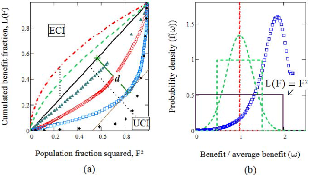
Figure 1. (a) Concave and convex L-graphs resulting from equal- and unequal-chance inequality, respectively. ─∙─ Perfect equality, $L\left(F\right)=F$. $——$ Gaussian and its Gini-equivalent uniform density, both having $Gi=0.17$—Equal-chance line, $L\left(F\right)=F²$. $▲▲▲$ USA incomes. $◦◦◦$ World electricity consumption. $▢▢▢$ Life expectation. ♦♦♦ Cancer rate of survival. Class boundaries, $F²=\frac{1}{4}$ and $L_2\left(F²\right)=1-F²$. –– Unit-slope tangent. X──X Distance d from equal-chance line. (b) Corresponding statistical distributions. Symbols apply as in (a).

Figure 1. (a) Concave and convex L-graphs resulting from equal- and unequal-chance inequality, respectively. ─∙─ Perfect equality, $L\left(F\right)=F$. $——$ Gaussian and its Gini-equivalent uniform density, both having $Gi=0.17$—Equal-chance line, $L\left(F\right)=F²$. $▲▲▲$ USA incomes. $◦◦◦$ World electricity consumption. $▢▢▢$ Life expectation. ♦♦♦ Cancer rate of survival. Class boundaries, $F²=\frac{1}{4}$ and $L_2\left(F²\right)=1-F²$. –– Unit-slope tangent. X──X Distance d from equal-chance line. (b) Corresponding statistical distributions. Symbols apply as in (a).

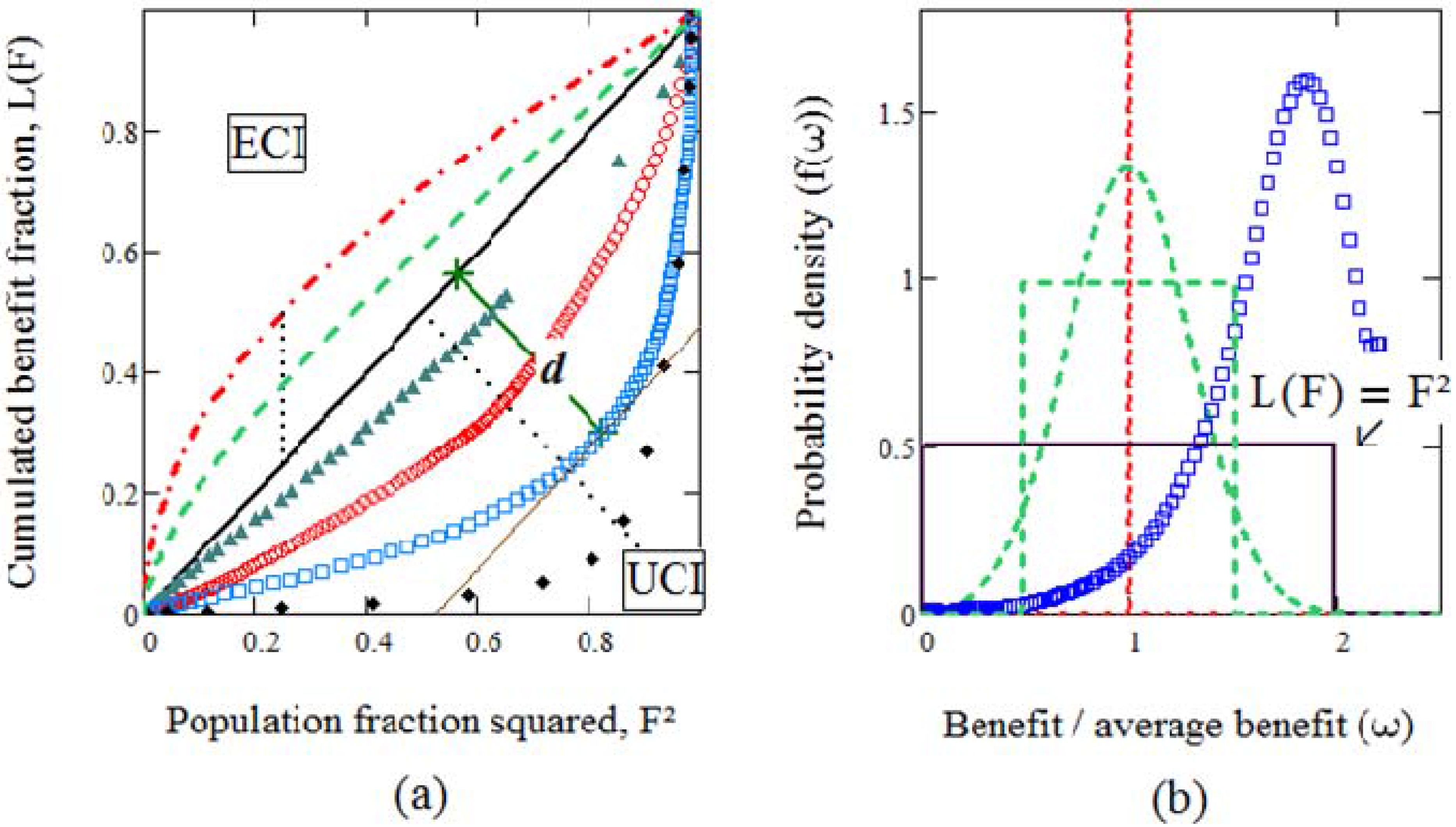
The unequal-chance inequality (UCI) region is defined by $F²>L_2\left(F²\right)$. Real-world data lies in this region and forms downward-concave L-curves. This is also the case of beer bubble-size distributions [23], that systematically show $Gi\ge 0.33$ and asymmetric PDFs. Of course, besides the common points (0,0) and (1,1), there is no possible intersection of concave and convex L-curves. The transition line, $L=F²$, implies $\omega =2F$ and an optimal uniform density $f_u\left(\omega \right)=\frac{1}{2}$, shown in Figure 1b.

2.2.2. Symmetry, Class Boundaries and Discontinuities

The median, the mode and the mean coincide for symmetrical distributions. The natural boundary between classes is then the axis of symmetry, as illustrated in Figure 1b, with $F_p=\frac{1}{2}$ and $\omega \left(F_p\right)=\langle \omega \rangle =1$. By Lemma 1 in the appendix, it coincides with a maximum of $\varphi =L_2\left(F²\right)-F²$. In fact, the extremums of $\varphi$ occur in both regions at points of abscissa $F_0^2$ where ${\frac{d{L}_2}{d\left(F²\right)}|}_{F_0^2}=1$, that is, where the tangent to $L_2\left(F²\right)$ is perpendicular to the second diagonal in Figure 1a, of equation $L_2\left(F_0^2\right)=1-F_0^2$. We therefore extend the definition of class boundary to the locus of all extremums of $\varphi$. We call $L_2\left(F_0^2\right)$ the ideal UCI class-boundary line, because it closely describes the minima of $\varphi$ in this region. Now, ECI extremums of $\varphi$ form a vertical line of abscissa $F_0^2=\frac{1}{4}$, while $\frac{1}{2}\le F_0^2\le 1$ in the UCI region. There is clearly a discontinuity in the values of $F_0^2$, a hint of a possible phase transition. Since $F_p$ must be continuous according to the generalised Pareto principle, we circumvent the difficulty by giving region-dependent definitions: $F_p=F_0=\frac{1}{2}$ in the ECI region and $F_p=F_0^2>\frac{1}{2}$ in the UCI region.

Inequality thus shows up in at least two conceivable and non equivalent ways: for ECI, the poor fraction of the population equals the rich fraction, $F_p=1-F_p$, but the former as a whole gets less than the latter, $L\left(F_p\right)<\frac{1}{2}<1-L\left(F_p\right)$; for UCI, one of the two classes outnumbers the other, $F_p>\frac{1}{2}>1–F_p$, with $F_p=1$ for absolute inequality. The generalised Pareto criterion results in $L\left(F_p\right)=1-F_p$ and, from Lemma 2 in the appendix, the maximum per capita benefit is necessarily greater than twice the average in this case.

2.3. Universality

If a phase transition is indeed at work here, we expect a law of corresponding states to apply, as it does for similar transformations in physics [12,13]. L-curves should result from one another by suitable rescaling of universal functions, at most one on each side of the transition line $L=F²$. This is shown in Figure 2 for symmetrical distributions in Figure 2a and empirical UCI data in Figure 2b. Gini-equivalent $\varphi$-curves from symmetrical distributions necessarily intersect an even number of times, twice in practice, on both sides of the axis of symmetry, as illustrated by Figure 2a. Figure 2b describes UCI and results from a rotation of axes by 45 degrees in Figure 1a, so as to make the F²-axis join the main diagonal, followed by (cosmetic) inversion of the resulting ordinates to make data positive. One obtains $\psi \left(X\right)$ graphs looking like the made-up dashed curve in Figure 2b, intersecting once the UCI universal curve. After normalisation and rescaling of the X-axis so as to have all $X_M$ coincident a $X_M=\frac{1}{2}$, empirical data crowds indeed close to a universal curve as shown in Figure 2b. The rotation results in new coordinates $\left(X,Y\right)$, where $Y\left(X\right)$ is the universal curve, defined parametrically in the UCI region by:

$$X=\frac{F²+L_2\left(F²\right)}{2},Y=\frac{F²-L_2\left(F²\right)}{d\sqrt{2}}=\frac{\psi \left(X\right)}{{\psi }_M}$$

(5)

where ${\psi }_M=d\sqrt{2}$ is the maximum of $\psi \left(X\right)$, with d the maximum distance between the $L=F²$ line and the L-curve.

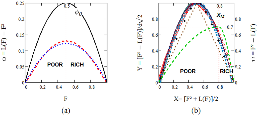
Figure 2. Symmetry-dependent universal behaviours. (a) ECI concave L-curves: ––Perfect equality, $Gi=0$. ∙∙∙∙ Uniform distribution, $R=0.33,Gi=0.17$. $–\; –\; –$ Gini-equivalent, Gaussian-like distribution, $Gi=\mathrm{0.17.}$ (b) UCI convex L-curves: $▲▲▲$ Incomes. $◦◦◦$ World electricity consumption. $▢▢▢$ Life expectation. ♦♦♦ Rate of survival after cancer. –– Theoretical curve. ∙∙∙∙∙ Absolute inequality. $-\; -\; -$ Fictitious data before normalisation and symmetrisation (right-hand ordinates, with $d\sqrt{2}=0.7,X_M=0.8$).

Figure 2. Symmetry-dependent universal behaviours. (a) ECI concave L-curves: ––Perfect equality, $Gi=0$. ∙∙∙∙ Uniform distribution, $R=0.33,Gi=0.17$. $–\; –\; –$ Gini-equivalent, Gaussian-like distribution, $Gi=\mathrm{0.17.}$ (b) UCI convex L-curves: $▲▲▲$ Incomes. $◦◦◦$ World electricity consumption. $▢▢▢$ Life expectation. ♦♦♦ Rate of survival after cancer. –– Theoretical curve. ∙∙∙∙∙ Absolute inequality. $-\; -\; -$ Fictitious data before normalisation and symmetrisation (right-hand ordinates, with $d\sqrt{2}=0.7,X_M=0.8$).

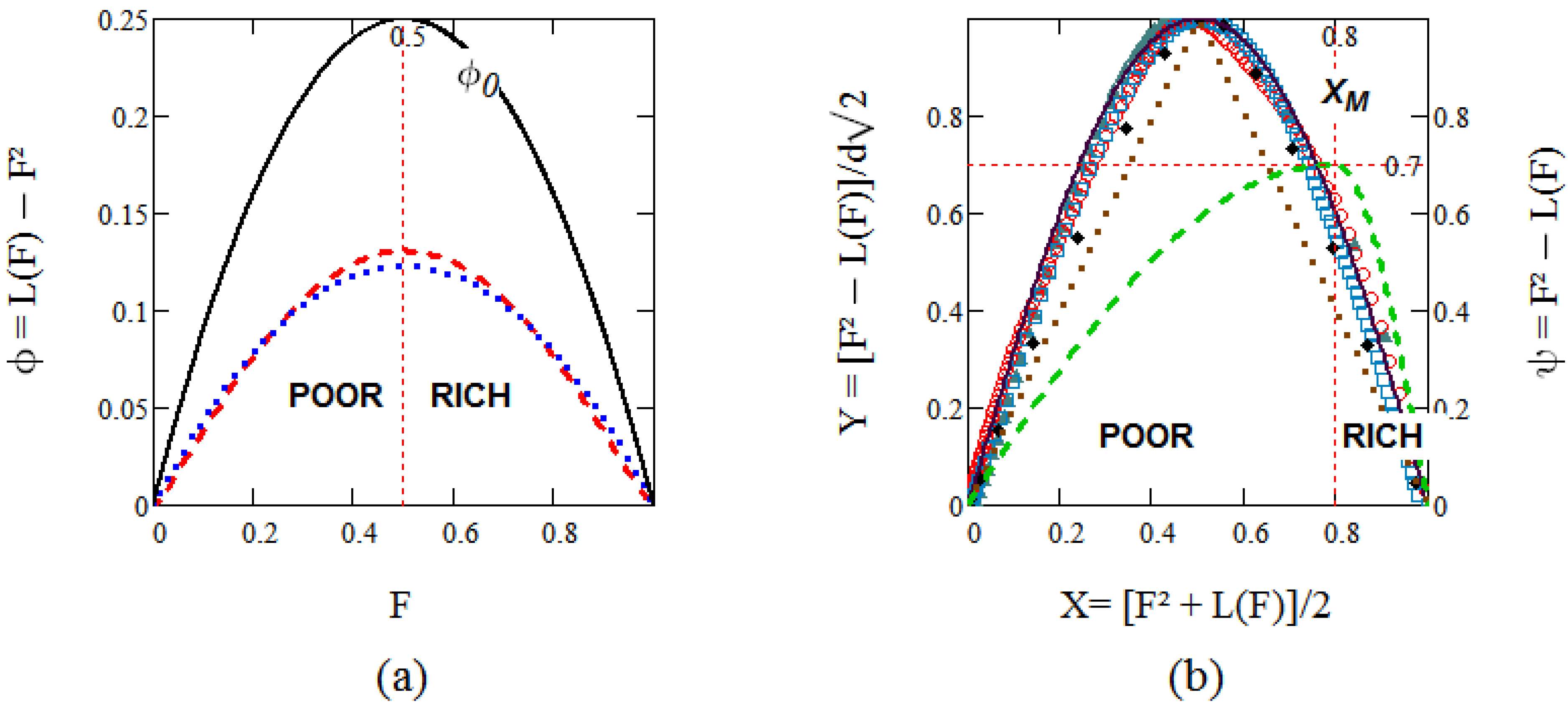
Data shows this maximum to occur at values $X_M\simeq \frac{1}{2}$ in all cases. The theoretical curve, to be obtained in the next section, is also shown for comparison. The L-curve for absolute inequality is just a pair of perpendicular straight lines, $L=0$ for $0\le F²<1$, and $0<L\le 1$ for $F²=1$, with $\sqrt{2}d=1$. It becomes $Y=F²=2X$ fo $X\le \frac{1}{2}$ and $Y=2\left(1-X\right)$ for $X>\frac{1}{2}$ in Figure 2b.

3. The Transition to Convexity

3.1. Probabilistic Model

We define the unequal-chance order parameter (OP) of the concave → convex transformation as the difference between equal- and unequal-chance cumulated benefit fractions for the population fraction $F$ in the UCI region, and zero elsewhere. It is just the numerator $\psi \left(X\right)={\psi }_{M}Y\left(X\right)=F²-L_2\left(F²\right)$ in the second Equation (5). Let $S\left\{\psi \right\}$ be the entropy functional an $S_0$ the entropy in the $L=F²$ equal-chance state. We assume that constraints exist that result in an entropy difference $S\left\{\psi \right\}-S_0<0$ that depends not only on $\psi \left(X\right)$, but also on $\frac{d\psi }{dX}$. Indeed, if correlations exist, they should depend on the gradient of the order parameter. The maximum ${\psi }_M=\psi \left(X_M\right)=\sqrt{2}d$ for each curve is the difference between the probability of being poor and that of being rich, ${\psi }_M\approx F_p-\left(1-F_p\right)=2F_0^2-1=\sqrt{2}d\le 1$. At absolute inequality ${\psi }_M=1$, $F_p=1$ and $S\left\{{\psi }_M\right\}=0$; thereon $S\left\{\psi \right\}$ increases as d decreases. Now, the asymmetry is the same if the poor outnumber the rich—the case of incomes—or just the opposite, as for demography, where the numerous young are richer in life expectation. The signs of the OP and its derivative should therefore be irrelevant. The Taylor expansion of the entropy density $\frac{dS}{dX}$ contains then only even powers of $\psi \left(X\right)$ and $\frac{d\psi }{dX}$. For $\psi \ll 1$, to fourth order in the OP and second order in its derivative we have:

$$\begin{array}{l}S\left\{\psi \right\}=S_0\left\{1+A{{\displaystyle \int }}_0^1\left[\psi ²+\frac{B}{A}{\psi }^4+\frac{C}{A}{\left(\frac{d\psi }{dX}\right)}^2\right]dX\right\}\\ =S_0\left\{1-4d²{{\displaystyle \int }}_0^1\left[Y^2-d^2{Y}^4-{\xi }^2{\left(\frac{dY}{dX}\right)}^2\right]dX\right\},\end{array}$$

(6)

where $\xi ²=-\frac{C}{A}$, and $A<0$ is required to make $S\left\{\psi \equiv 1\right\}=0$, while $\psi \left(X\right)\ne 0$ must optimise the integral. Note the great generality of this approach. It applies equally well to any type of entropic form out of the many that have been proposed, whether extensive or not [24]. Equation (6) could also conceivably describe average entropy production, for example. Anyway, these undefined features do not prevent the calculation to proceed.

3.1.1. Entropy Maximisation

At first sight, three parameters, $A, B, C$, are necessary to describe a single L-curve, but Figure 2b suggests that at most two parameters, d and eventually $X_M$, should suffice. Consider then two cases where we know that $\psi$ is a constant, the equal chance limit with $\psi \to 0$, and absolute inequality with $\psi \to 1$ and $S\left\{1\right\}=0$. According to the definition, $S=S_0$ for arbitrary $A$ or $B$ in the entire ECI region, which results in $\psi =0\ne -\varphi$ in it. Maximum entropy requires $\psi \left(A+2B{\psi }^2\right)=0$, so $\psi ={\psi }_M$ is either zero, as expected for the first case, or $\sqrt{\frac{-A}{2B}}=1$ in the second case, i.e. $A=-2$ and $B=1$. We tentatively apply these values to the whole UCI region. Incidentally, if L-curves rather than straight lines are to be obtained, this is a matter-of-fact argument for the introduction of the derivative term. The condition for an extremum is given by Euler’s equation, which reads:

$$\xi ²\frac{d²Y}{dX²}+Y\left(1-2d²Y^2\right)=0,$$

(7)

with boundary conditions $Y\left(X_M\right)=1, Y^{\prime }\left(X_M\right)={\left(\frac{dY}{dX}\right)|}_{X_M}=0$, supplemented by $Y\left(0\right)=Y\left(1\right)=0$. Useful insight is obtained from successive approximate solutions. All boundary conditions are satisfied in the $d\to 0^{+}$ limit by $Y\left(X\right)=\sin \left(\frac{X}{{\xi }_0}\right), {\xi }_0=\frac{1}{\pi }$. When replaced in (6) this solution makes the integral equal to zero as announced, independently of the value of $A$. Next, we linearise Equation (7) by replacing $Y^2$ by its average in the previous approximation, $\langle \sin ²\left(\frac{X}{{\xi }_0}\right)\rangle =\frac{1}{2}$. Now, if $Y$ is indeed universal it cannot depend on d, which imposes $\xi ={\xi }_0\sqrt{1-d²}$. The parameter $\xi$ is a natural unit of measurement of $X$ and of the rate of change of the OP, insofar as a sizeable change in the latter along an L-curve requires significant changes in the ratio $\frac{X}{\xi }$. Schematically, it defines a cohesion range on $X$ such that increments $\mathsf{\Delta }X\ll \xi$ are unimportant, those where $\mathsf{\Delta }X\gg \xi$ do matter, and a significant level of equality of chances persists for $\mathsf{\Delta }X\approx \xi$. The product $\pi \xi$ furnishes a convenient correlation or cohesion indicator: it is a maximum, unity, for minimum UCI, $\left(d=0^{+}\right)$, and decreases to zero, as shown below, for absolute inequality ($\sqrt{2}d=1$). Equation (7) admits a first integral:

$${\xi }^2{\left(\frac{dY}{dX}\right)}^2+Y^2-d^2{Y}^4=1-d^2={\xi }^2{{\left(\frac{dY}{dX}\right)}^2|}_{X=0}={\xi }^2{{\left(\frac{dY}{dX}\right)}^2|}_{X=1}.$$

(8)

3.1.2. Class Asymmetry and Intersections of L-Curves

If $\psi \left(X\right)$ is not strictly symmetrical about$X_M=\frac{1}{2}$, the two derivatives at the end of (8) will be different, which requires two values of $\xi$ for a single value of d. We use the notation ${\xi }_{p|r}=\left\{{\xi }_p\text{|}{\xi }_r\right\}$ for a simultaneous description of the two classes. The approximate solution found for Equation (7) above suggests putting $Y=\sin \phi$. When this is replaced in Equation (8), its solution can be expressed in parametric form, in terms of the incomplete, $\mathsf{\Phi }\left(k²,\phi \right)$, and complete, $K\left(k²\right)=\mathsf{\Phi }(k²,\frac{\mathsf{\pi }}{2})$, elliptic integrals of the first kind [25], with $k²=\frac{d²}{1-d²}$:

$$X_{p|r}\left(k²,\phi \right)=\left\{\frac{\mathsf{\Phi }\left(k^2,\phi \right)}{K\left(k²\right)}{X}_M|X_M+\frac{\mathsf{\Phi }\left(k^2,\phi -\frac{\pi }{2}\right)}{K\left(k²\right)}\left(1-X_M\right)\right\},Y=\sin \phi$$

(9)

and:

$$\mathsf{\Phi }\left(k²,\phi \right)={{\displaystyle \int }}_0^{\phi }\frac{1}{\sqrt{1-k²\text{sin}²\theta }}d\theta ,\phi \le \frac{\pi }{2}.$$

(10)

Its continuation into the region $\pi \ge \phi >\frac{\pi }{2}$ is just $\mathsf{\Phi }\left(k²,\phi \right)=K\left(k²\right)+\mathsf{\Phi }\left(k²,\phi -\frac{\pi }{2}\right)$. The cohesion ranges are:

$${\xi }_{p|r}\left(k²\right)=\frac{1}{K\left(k^2\right)\sqrt{1+k²}}\left\{X_M\text{|}1-X_M\right\}=2\xi \left(k²\right)\left\{X_M\text{|}1-X_M\right\}$$

(11)

One recovers the approximate expression for ${\xi }_0=\frac{1}{2K\left(0\right)}=\frac{1}{\pi }$ obtained above. Equation (11) shows that the average parameter $\xi \left(k²\right)=\frac{{\xi }_p+{\xi }_r}{2}=\frac{1}{2K\left(k²\right)\sqrt{1+k²}}$, describing the interclass cohesion, is a decreasing function of k² that becomes $\xi \left(1\right)=0$ at absolute inequality, where no cohesion is possible. Class asymmetry is defined by $\mathsf{\Delta }=\frac{{\xi }_p-{\xi }_r}{{\xi }_p+{\xi }_r}=2X_M-1$. If $\mathsf{\Delta }\ne 0$, two parameters, like d and $X_M$, ${\xi }_p$ and ξ_r, or $\xi \left(k²\right)$ and $\mathsf{\Delta }$, suffice to characterise an L-curve. As a result two convex L-curves, say A and B, having (i) $d_A=d_B$, coincide if $X_{M,A}=X_{M,B}$; they intersect once if $X_{M,A}\ne X_{M,B}$. In both cases $G{i}_A=G{i}_B$. (ii) If $d_A\ne d_B$ intersections are irrelevant because in all cases $G{i}_A\ne G{i}_B$, but there is no intersection if $X_{M,A}=X_{M,B}$. The apparent dependence of $X\left(k²,\phi \right)$ on k² is in fact negligible over the range of interest. The universal curve in Figure 2b makes use of the average $\langle k²\rangle =0.139$ and provides an acceptable fit to all our data.

4. Results

4.1. Fitting Empirical Data

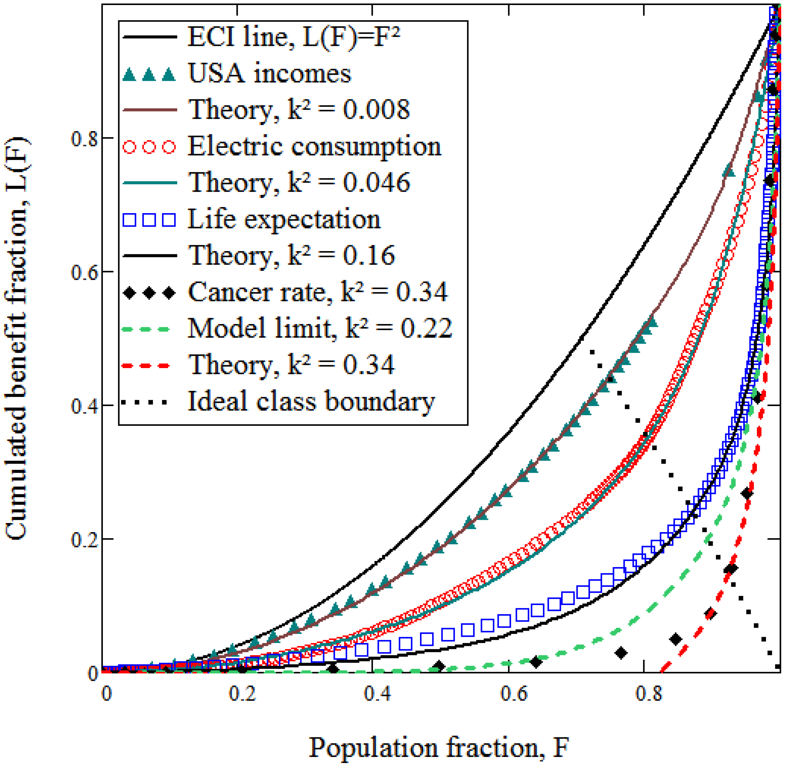
Equations (5), once solved for $F$ and $L_2\left(F^2\right)$ as functions of $X$ and $Y$, allow, using Equation (9), to obtain theoretical Lorenz curves in the UCI region. The parameters $d$ and $X_M$ are directly read from data—i.e., not adjusted for an overall fit. They provide Lorenz curves as shown in Figure 3a conventional $L\left(F\right)$ plot. The expansion in Equation (6) is in principle valid only for $\psi \ll 1$. A distinctive feature of this model is that it precisely defines its own limit, $k²=0.22$, above which the theoretical initial slope of $L_2\left(F²\right)$ becomes unrealistically negative, as suggested by Figure 3. Universality of L-curves is nevertheless substantiated well beyond this limit, as shown in Figure 2, where cancer data has $k²=0.34$.

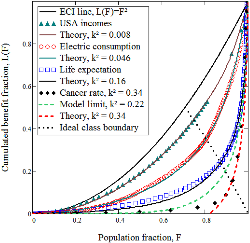
Figure 3. Conventional $L\left(F\right)$ Lorenz plots. Symbols for data and for their fits by model predictions are shown in the insert. The model should not apply for values $k²>0.22$.

Figure 3. Conventional $L\left(F\right)$ Lorenz plots. Symbols for data and for their fits by model predictions are shown in the insert. The model should not apply for values $k²>0.22$.

4.2. A New Indicator

The main advantage of the Gini coefficient is its conceptual simplicity, though counterbalanced by possible inaccuracies when obtained from discontinuous data. Equations (5) and (9) provide a function describing L-curves and thereby allow a precise numerical integration of the function $F-L\left(F\right)$ in Equation (3). Gini values in Table 1 below have been obtained in this way. Furthermore, a new Gini-like indicator $G{i}_{uc}$, measures unequal-chance inequality in the $\left(F^2,L_2\right)$ plane, and is easily obtained in closed form. It is twice the area under the curve $\psi =F²-L_2\left(F²\right)=\sqrt{2}d\sin \phi$:

$$\begin{array}{l}G{i}_{uc}\left(k\right)=2\sqrt{2}d{{\displaystyle \int }}_0^{\mathsf{\pi }}Y\left(X\right)\frac{dX}{d\theta }d\theta \\ =\frac{2}{K\left(k^2\right)}\sqrt{\frac{2}{1+k^2}}{{\displaystyle \int }}_0^{\frac{\pi }{2}}\frac{k\sin \theta }{\sqrt{1-k^2{\text{sin}}^2\theta }}d\theta \\ =2\sqrt{\frac{2}{1+k^2}}\frac{\text{argth}\left(k\right)}{K(k^2)},k²\le \mathrm{0.22.}\end{array}$$

(12)

Quantities like $Gi$ and $G{i}_{uc}\left(k\right)$, resulting from a good fit to the whole L-curve, become meaningless for $k²>0.22$. Others, dependent on the single value d through $k²=\frac{d²}{1-d²}$ like $\xi \left(k²\right)$, are still valid beyond this limit. This is shown in Table 1.

Table 1. Characteristic parameters of unequal-chance inequality for different types of data. $F_p$ is the largest fraction of the population, the poorest in the first two cases, the youngest in the other two.

BENEFIT	k2	FP	XM	$\mathit{d}\sqrt{\mathbf{2}}$	$\mathit{\pi }\mathit{\xi }\left(\mathit{k}\mathbf{²}\right)$	$\mathsf{\Delta }=\frac{{\mathit{\xi }}_{\mathit{p}}-{\mathit{\xi }}_{\mathit{r}}}{{\mathit{\xi }}_{\mathit{p}}+{\mathit{\xi }}_{\mathit{r}}}$	$\mathit{G}\mathit{i}$	Giuc(k)
Income	0.008	0.58	0.68	0.16	0.99	0.35	0.46	0.16
Electricity consumption	0.046	0.66	0.52	0.32	0.97	0.04	0.60	0.38
Life expectation	0.159	0.76	0.55	0.52	0.89	0.10	0.79	0.68
Model limits	0.220	0.80	0.5	0.60	0.85	0	0.85	0.78
Survival after cancer	0.344	0.86	0.45	0.71	0.78	–0.11	––	––

Table 1. Characteristic parameters of unequal-chance inequality for different types of data. $F_p$ is the largest fraction of the population, the poorest in the first two cases, the youngest in the other two.

BENEFIT	k2	FP	XM	$\mathit{d}\sqrt{\mathbf{2}}$	$\mathit{\pi }\mathit{\xi }\left(\mathit{k}\mathbf{²}\right)$	$\mathsf{\Delta }=\frac{{\mathit{\xi }}_{\mathit{p}}-{\mathit{\xi }}_{\mathit{r}}}{{\mathit{\xi }}_{\mathit{p}}+{\mathit{\xi }}_{\mathit{r}}}$	$\mathit{G}\mathit{i}$	Giuc(k)
Income	0.008	0.58	0.68	0.16	0.99	0.35	0.46	0.16
Electricity consumption	0.046	0.66	0.52	0.32	0.97	0.04	0.60	0.38
Life expectation	0.159	0.76	0.55	0.52	0.89	0.10	0.79	0.68
Model limits	0.220	0.80	0.5	0.60	0.85	0	0.85	0.78
Survival after cancer	0.344	0.86	0.45	0.71	0.78	–0.11	––	––

5. Conclusions

This work provides a model that fairly fits Lorenz curves, up to $Gi=0.85$. It is just the social analogue of Ginzburg and Landau’s ideas [13] on second-order phase transitions in physics. The symmetry of the statistical distribution plays a crucial role in this development. Symmetrical distributions result in ECI downward-concave $L_2\left(F²\right)$ curves, $Gi<\frac{1}{3}$ and $w_m+w_M=2\langle w\rangle$, i.e., nobody gets more than twice the per capita average, a straightforward but apparently overlooked result. Since equality of chances must be a rather unusual event, too low values of $Gi$ may be profitably checked for consistency against this relation. Asymmetrical distributions display convex L-curves, $Gi>\frac{1}{3}$ and impose $w_M>2\langle w\rangle$. Initial slopes of $L_2\left(F²\right)$ furnish a supplementary criterion, though less convenient for numerical applications. A clear-cut distinction appears to be necessary between equal- and unequal-chance inequalities, related to different regions in the $\left(F², L_2\right)$ plane. One may expect that critical values, corresponding to $Gi=\frac{1}{3}$ at the phase transition, will also be found in other indicators of inequality. New parameters appear in the UCI region, like the cohesion range $\xi$, measuring the range of persistent equality in the distribution, the asymmetry parameter $\mathsf{\Delta }$, and the Gini-like coefficient $G{i}_{uc}$. The latter measures how far away a society is from maximum ECI in just the same way as $Gi$ measures how far away it is from perfect equality.

Quite different phenomena, from income distribution to cancer rate of survival, obey the same statistical laws. The resulting description of inequality implies an apparently oversimplified two-class division of society. A more detailed analysis should provide criteria allowing recognition of existing classes, whatever their number, out of real-life distributions. This amounts to a nontrivial challenge – modelling the probability density function.

References

- Lorenz, M.O. Methods of measuring concentration of wealth. J. Amer. Statist. Assoc. 1905, 9, 209–219. [Google Scholar] [CrossRef]
- Gini, C. Variabilità e mutabilità (1912). In Memorie di Metodologia Statistica; Pizetti, E., Salvemini, T., Eds.; Libreria Eredi Virgilio Veschi: Rome, Italy, 1955. [Google Scholar]
- Rosenblatt, J.; Martinas, K. Inequality indicators and distinguishability in economics. Physica. A 2008, 387, 2047–2054. [Google Scholar] [CrossRef]
- Rosenblatt, J.; Martinas, K. Probabilistic foundations of economic distributions and inequality indicators. In Income Distribution: Inequalities, Impacts and Incentives; Irving, H.W., Ed.; Nova Science Publishers: New York, NY, USA, 2008; pp. 149–170. [Google Scholar]
- Chakrabarti, B.K.; Chakraborti, A.; Chakravarty, S.R.; Chatterjee, A. Econophysics. of Income and Wealth Distributions; Cambridge University Press: Cambridge, UK, 2013. [Google Scholar]
- Souma, W. Physics of Personal Income, 2002. Available online: http://arxiv.org/cond-mat/0202388/ (accessed on: 08/01/13).
- Martinás, K. Thermodynamics and sustainability: A new approach by extropy. Per. Pol. Chem. Eng. 1998, 42, 69–83. [Google Scholar]
- Georgescu-Roegen, N. The Entropy Law and the Economic Process; Harvard University Press: Cambridge, MA, USA, 1971. [Google Scholar]
- Theil, H. Economics and Information Theory; North Holland: Amsterdam, The Netherlands, 1967. [Google Scholar]
- Eliazar, I. Randomness, evenness, and Rényi’s index. Physica A 2011, 390, 1982–1990. [Google Scholar] [CrossRef]
- Eliazar, I.; Sokolov, I.M. Measuring statistical evenness: A panoramic overview. Physica A 2012, 391, 1323–1353. [Google Scholar] [CrossRef]
- Landau, L. Theory of phase transitions (Part 1). Phys. Z. Sowjetunion. 1937, 11, 26, and (Part 2). Phys. Z Sowjetunion. 1937, 11, 545. [Google Scholar]
- Ginzburg, V.L.; Landau, L.D. On the theory of superconductivity. Zh. Eksp. Teor. Fiz. 1950, 20, 1064–1082. [Google Scholar]
- Pirjol, D. Phase Transition in a log-normal Markov Functional Model. J. Math. Phys. 2010, 52, 013301. [Google Scholar] [CrossRef]
- Atkinson, A.B. On the Measurement of Inequality. J. Econ. Theory 1970, 2, 244–263. [Google Scholar] [CrossRef]
- U.S. Census Bureau. Current Population Survey, Annual Social and Economic Supplement, 2007. Available online: http://www.census.gov/#/ (accessed on 4 February 2013).
- United Nations Development Programme. Available online: http://www.undp.org/ (accessed on 8 January 2013).
- New York City Cancer Statistics. Available online: http://www.health.state.ny.us/statistics/ cancer/registry/table6/tb6totalnyc.htm/ (accessed on 8 January 2013).
- Cowell, F.A. Measurement of inequality. In Handbook of Income Distribution; Atkinson, A.B., Bourguignon, F., Eds.; North Holland: Amsterdam, The Netherlands, 1999. [Google Scholar]
- Cohen, M.H.; Eliazar, I. Econophysical visualization of Adam Smith’s invisible hand. Physica A 2013, 392, 813–823. [Google Scholar] [CrossRef]
- Roemer, J. Equality of Opportunity; Harvard University Press: Cambridge, MA, USA, 1998. [Google Scholar]
- Yitzhaki, S.; Schechtman, E. The Gini. Methodology; Springer: New York, NY, USA, 2012. [Google Scholar]
- Sauerbrei, S. Lorenz curves, size classification, and dimensions of bubble size distributions. Entropy 2010, 12, 1–13. [Google Scholar] [CrossRef]
- Tsallis, C. Introduction to Nonextensive. Statistical Mechanics; Springer Science+Business Media: New York, NY, USA, 2009. [Google Scholar]
- Abramowitz, M.; Stegun, I. Handbook of Mathematical Functions; Dover: New York, NY, USA, 1972. [Google Scholar]
© 2013 by the authors; licensee MDPI, Basel, Switzerland. This article is an open access article distributed under the terms and conditions of the Creative Commons Attribution license (http://creativecommons.org/licenses/by/3.0/).