3.1. Chemical Equilibrium
The conversion of fuel into the oxidation products CO
2 and H
2O is subject to the chemical equilibrium constraint. Assuming that the reactants’ residence time is high enough in comparison with the characteristic chemical kinetics times (catalysis may be necessary), the chemical composition of the gas stream at the reduction reactor’s outlet can be determined as a function of temperature from the chemical equilibrium equation:
where
is the standard Gibbs’ function of reaction at temperature
T, and the equilibrium constant
can be related to the molar fractions of gases at equilibrium.
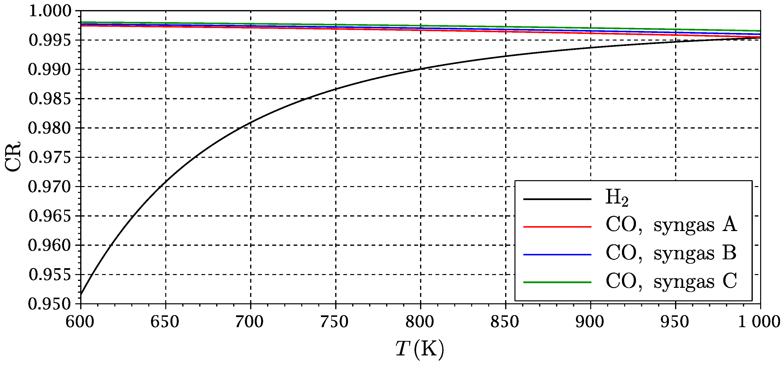
The conversion ratio of fuel as a function of temperature has been calculated. Results are shown in
Figure 4, where the conversion ratio has been defined as:
where
and
are
j’s initial molar fraction in syngas and its molar fraction at the chemical equilibrium. The dependence of the conversion ratio on pressure is very slight due to the conservation of the number of gas moles in both reactions (
4). In addition, as
for all considered syngas compositions, the curves for
result in being completely indistinguishable. Only one of them is printed in
Figure 4.
The conversion ratio of hydrogen increases with temperature, according to Le Châtelier’s principle, since the first reaction of (
4) is endothermic. In the case of carbon monoxide, a minor decrease with temperature (the second reaction of (
4) is slightly exothermic) can be observed and is somewhat higher for the fuels with a lower content of carbon dioxide, as this has a certain influence on the equilibrium condition. Unlike with conventional combustion, the fuel cannot be completely converted due to the equilibrium restrictions, but
Figure 4 shows that for a reaction temperature of around
, H
2’s conversion ratio reaches
and CO’s one is located at about 99.7–99.8% for all fuels. Thus, at this temperature, only approximately 0.55% of the fuel’s chemical exergy would be lost as a result of incomplete combustion. However, this effect is more than offset by the lower exergy destruction in the combustion process, as will be discussed in
Section 3.4.
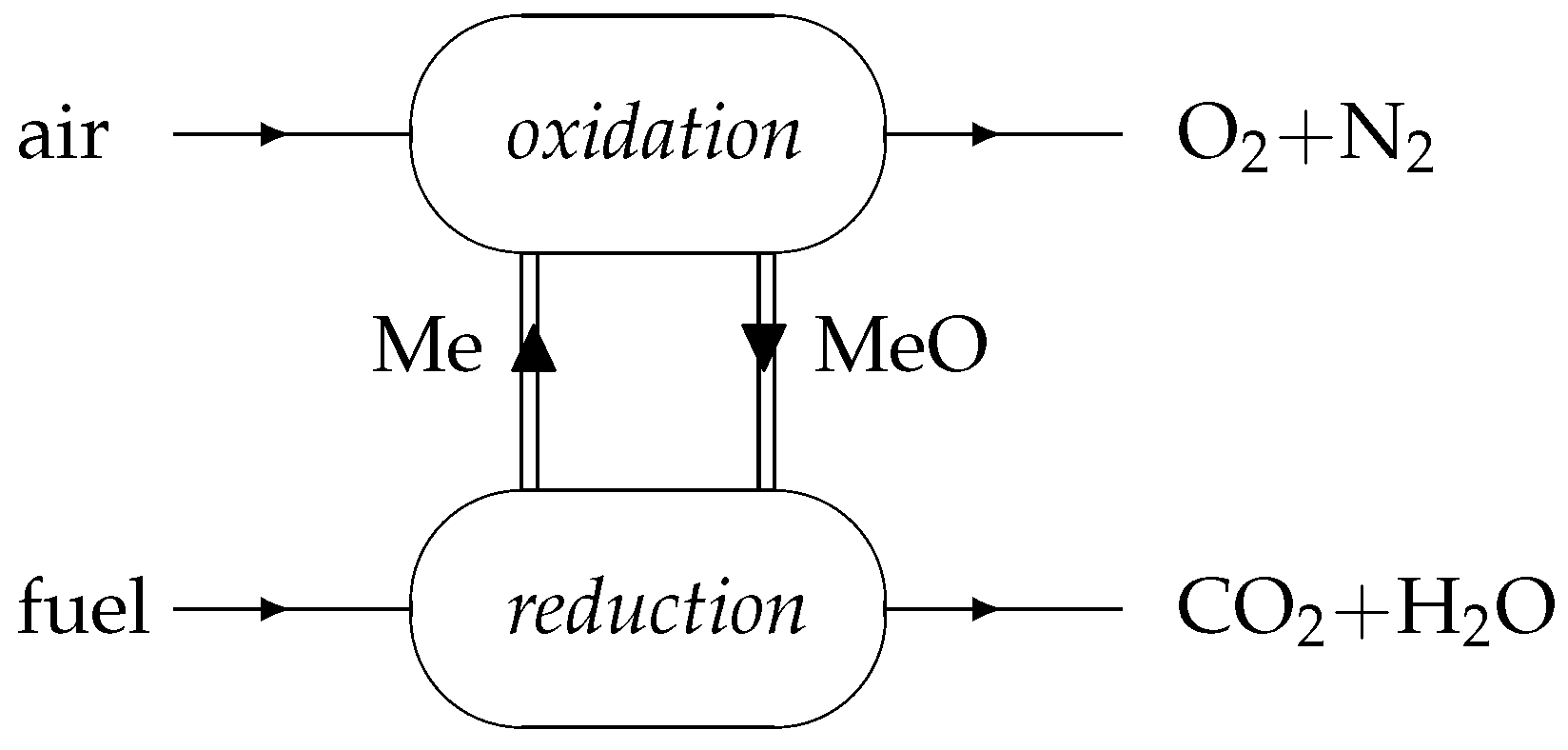
Regarding the oxidation reactor, chemical equilibrium has been found to never occur, as equilibrium would be attained for a really small oxygen molar fraction, much below the available oxygen in the reactor. All FeO is oxidized before that point.
3.2. Cycle Optimization and Exergy Efficiency
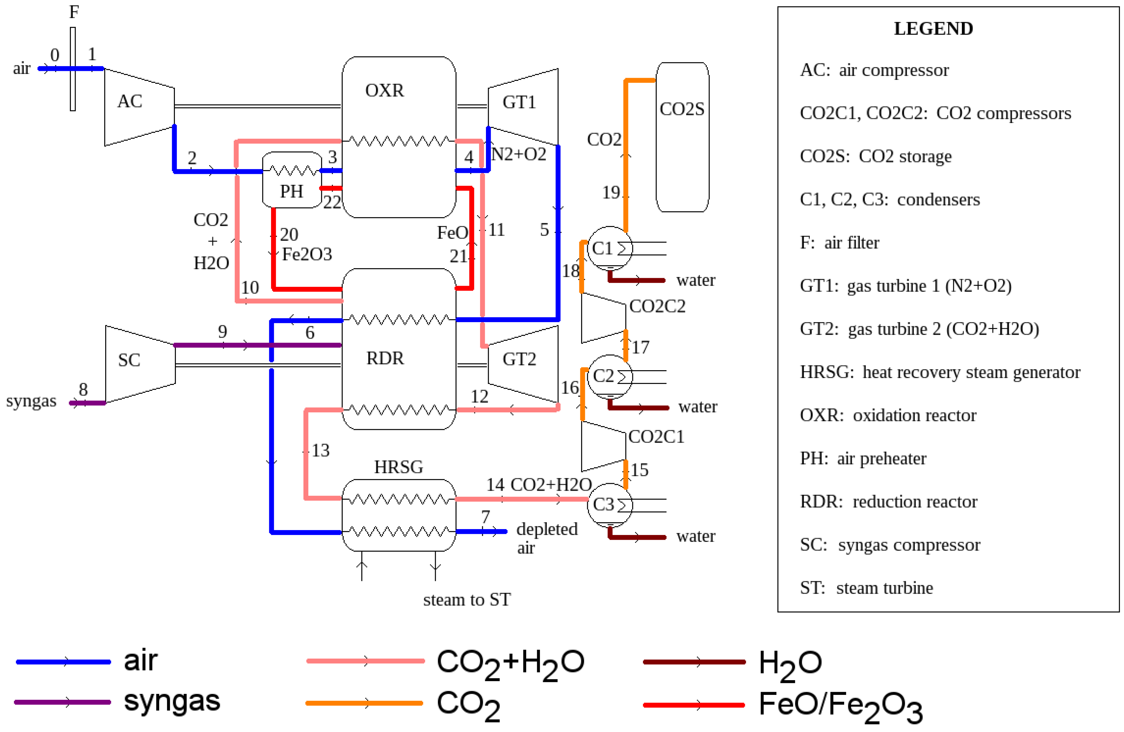
Few parameters define the thermodynamic conditions of the proposed power plant cycle (
Figure 2). The governing ones are the gas turbine GT1’s TIT (which also is the temperature of the oxidation reactor) and the reactors pressure
.
There is a degree of freedom about the reduction reactor temperature . This is the key parameter to be optimized in the cycle design. As discussed previously, the conversion ratio of hydrogen increases with the reactor’s temperature. However, this temperature is limited as the reduction reactor must take the required heat from the gas streams at the gas turbines’ outlets. An iterative algorithm has been implemented to calculate as the highest temperature possible that allows one to satisfy the energy balance in the reduction reactor.
There is a second degree of freedom of low importance in relation to the expansion pressure at the GT2 outlet (Stream 12). Calculations show that the pressure that gives the best ratio between the power developed by GT2 and the power consumed by the CO2 compressors is very close to for all fuels, but the influence on the results is minor in a broad range.
The cycle performance is evaluated from an exergetic point of view. The exergy efficiency is given by:
is the power generated by GT1, subtracting the air compressor power consumption,
is the power generated by GT2 minus the fuel compressor consumption,
is the power produced by the steam turbine and
is the power consumption of both CO
2 compressors:
A electromechanical efficiency for gas turbine ensembles of has been considered. is calculated in a similar way.
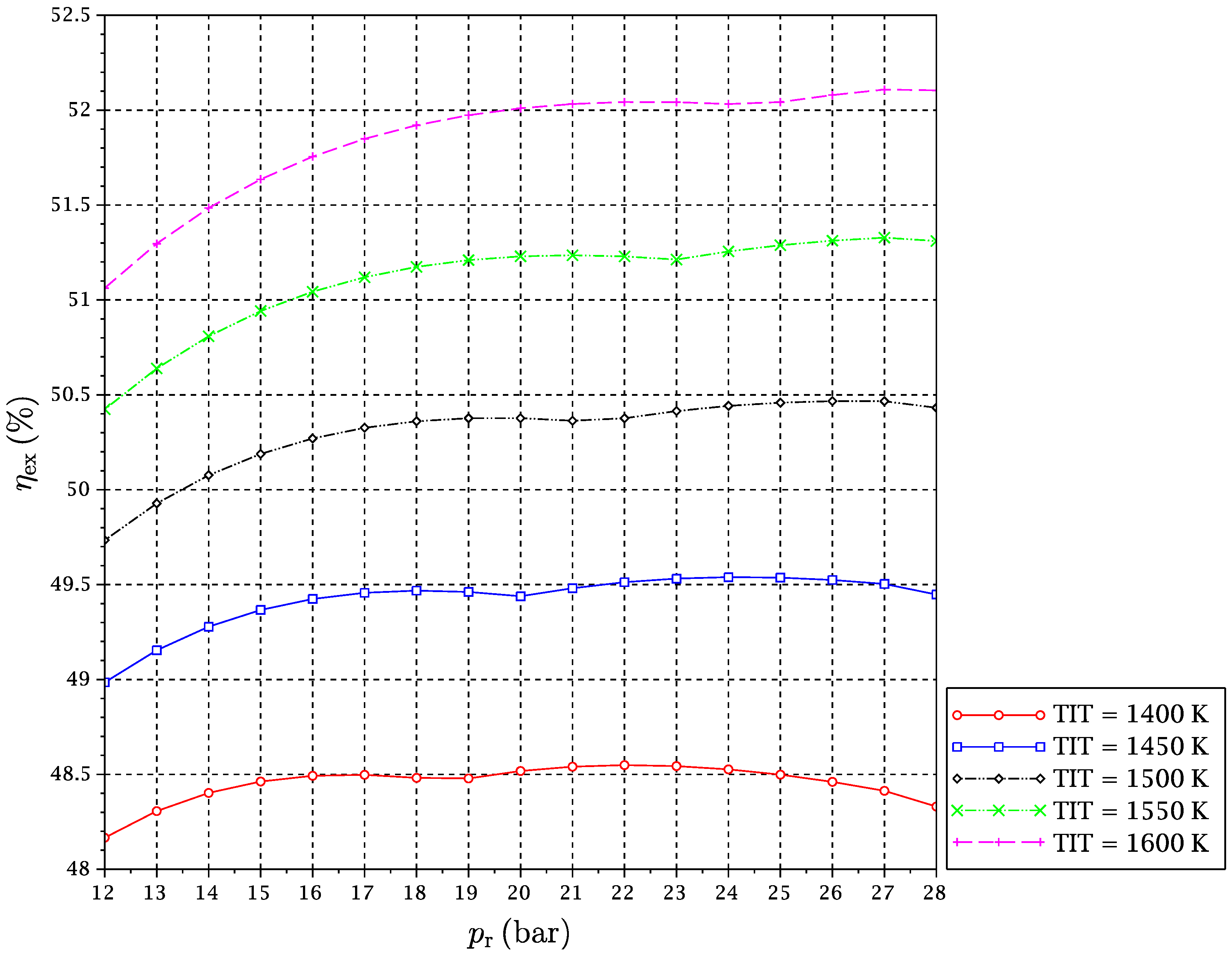
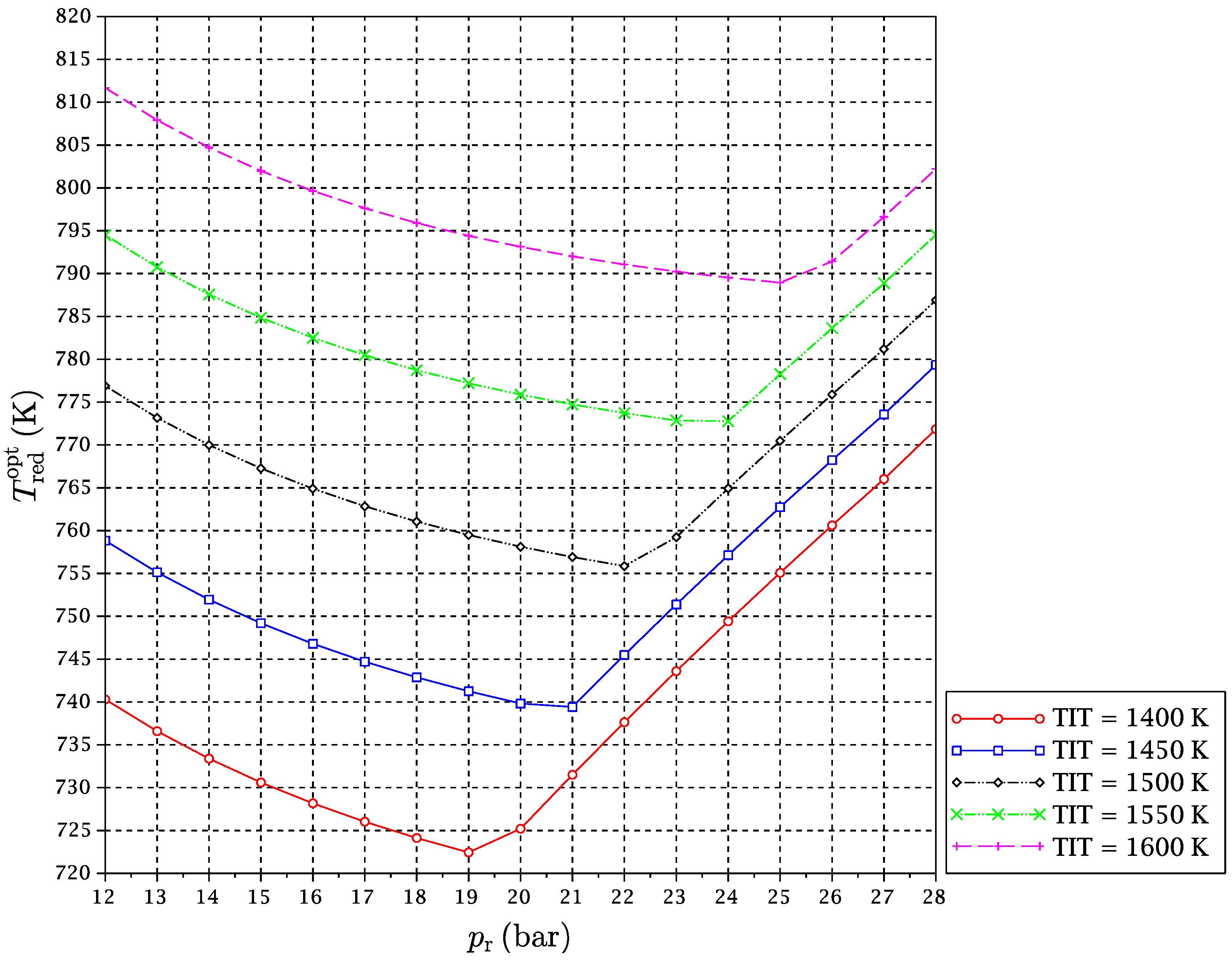
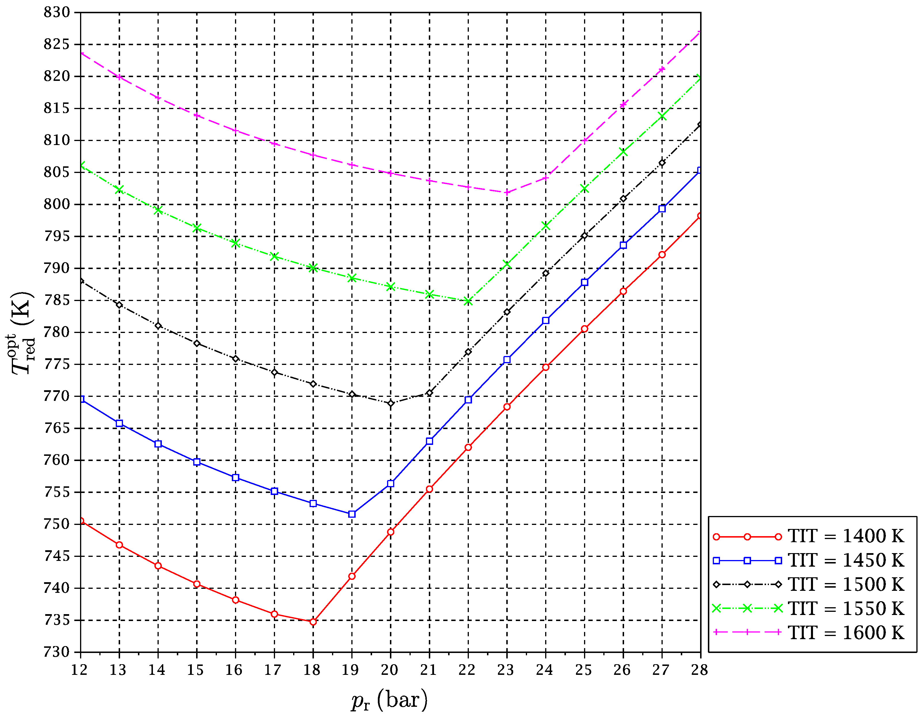
A set of simulations for TIT in a range from 1400–1600 K and
from 12–28 bar has been carried out. For each considered fuel and for every pair of values of TIT and
, the optimal reduction temperature and the exergy efficiency of the cycle have been obtained. Results are given in
Figure 5,
Figure 6,
Figure 7,
Figure 8,
Figure 9 and
Figure 10.
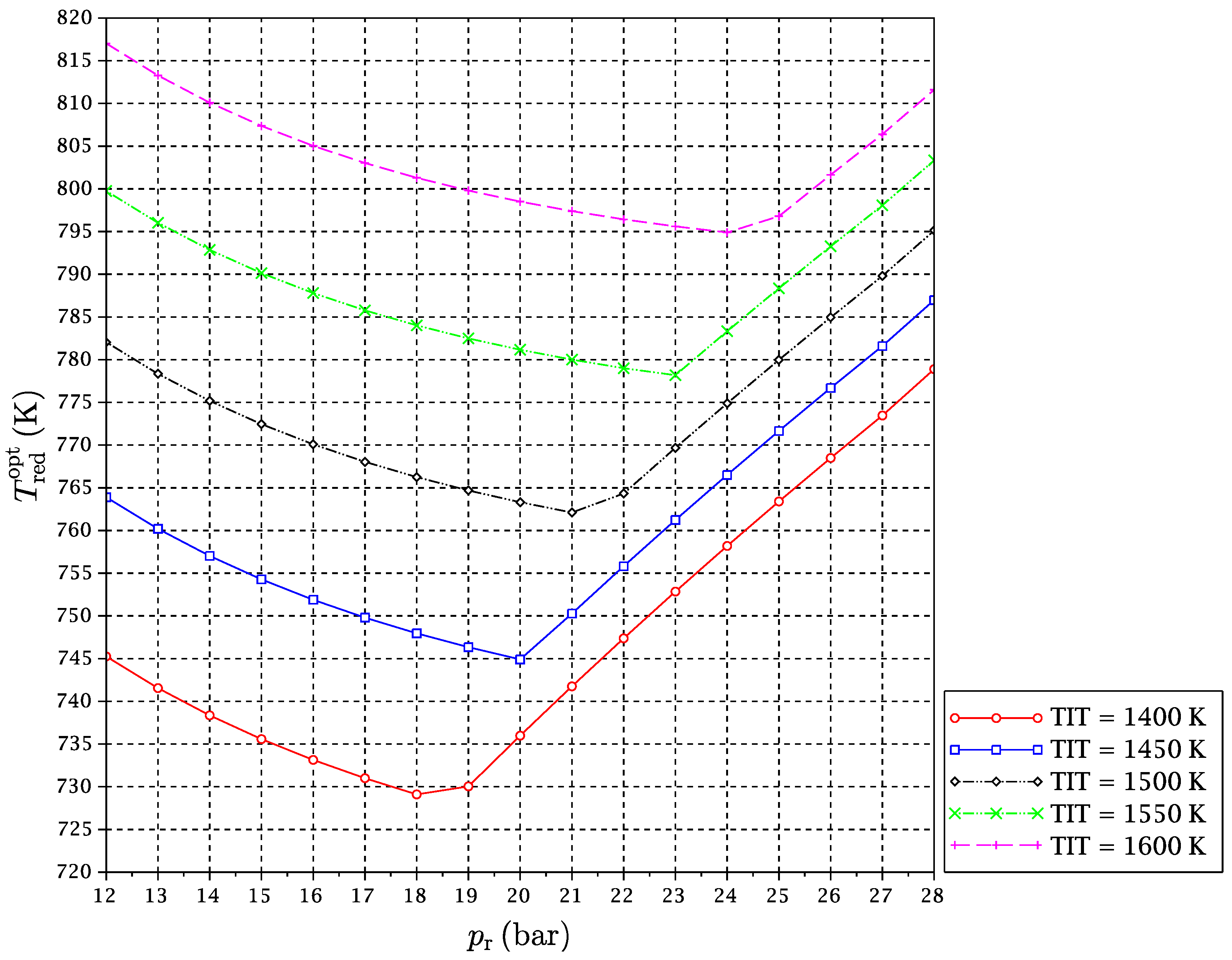
It might be interesting to expand on the freaky thermodynamic behavior revealed by these figures. A change in the tendency of the optimal temperature of the reduction reaction with
for a given TIT is observed. In principle, increasing the pressure ratio makes the gas turbines outlet temperature after expansion go down. For this reason, at low pressure ratios, the
is reduced with a pressure ratio increase, so that the reactor is able to take sufficient heat from the exhaust gas streams outgoing from the turbines to satisfy the energy balance. However, there is another opposing effect. The increment of pressure ratio compression leads to higher temperatures at the compressors outlets, which implies that the inputs to the reduction reactor are received there at higher temperatures. In summary, the following two effects occur at the same time when the reactors’ pressure is increased:
- (a)
Lower temperature of gas streams at the outlet of the gas turbines.
- (b)
A decrease of heat demand in the reduction reactor.
At some point, (b)-effect begins to dominate against (a)-effect. At a particular pressure, the heat needed by the reactor is decreased to a point that it can be provided by the CO
2 + H
2O stream only: the air stream results to uncouple from the reduction reactor heating. This can be seen somehow as a typical “power heat pump” effect (Do not confuse this effect with the so-called “chemical heat pump” effect discussed in
Section 1.1. The “power heat pump” effect refers just to the coming back of the energy that was introduced in the cycle as mechanical power in the air compressor as heat provided to the reduction reactor. The exergy content of this heat flow is then amplified by the “chemical heat pump” effect). Due to the complex heat coupling of streams and reactors in the CLC cycle, this allows
to reverse its trend, and it begins to increase with pressure ratio (
Figure 8,
Figure 9 and
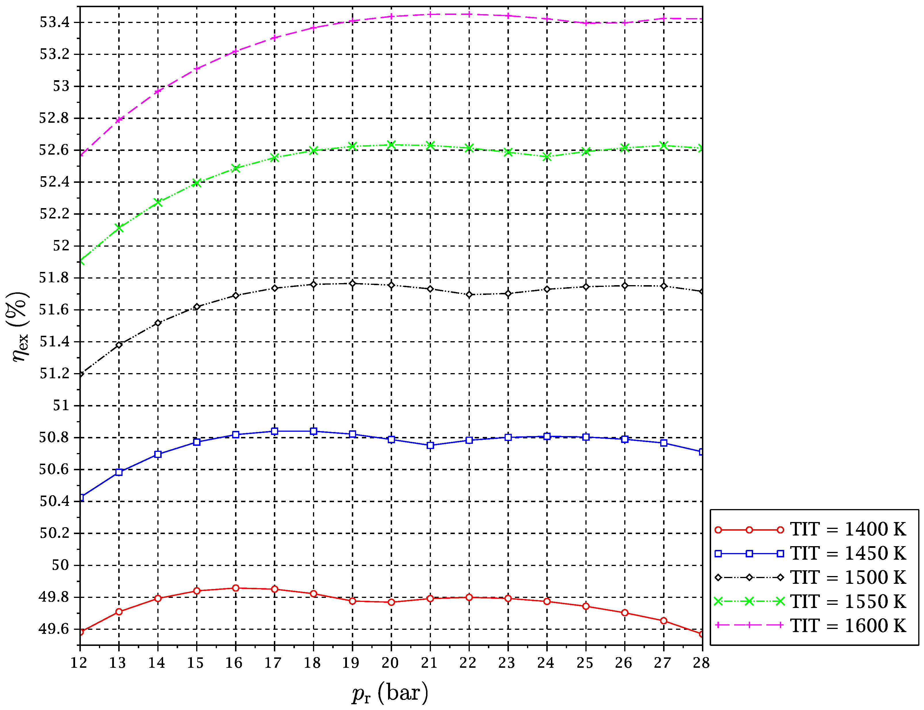
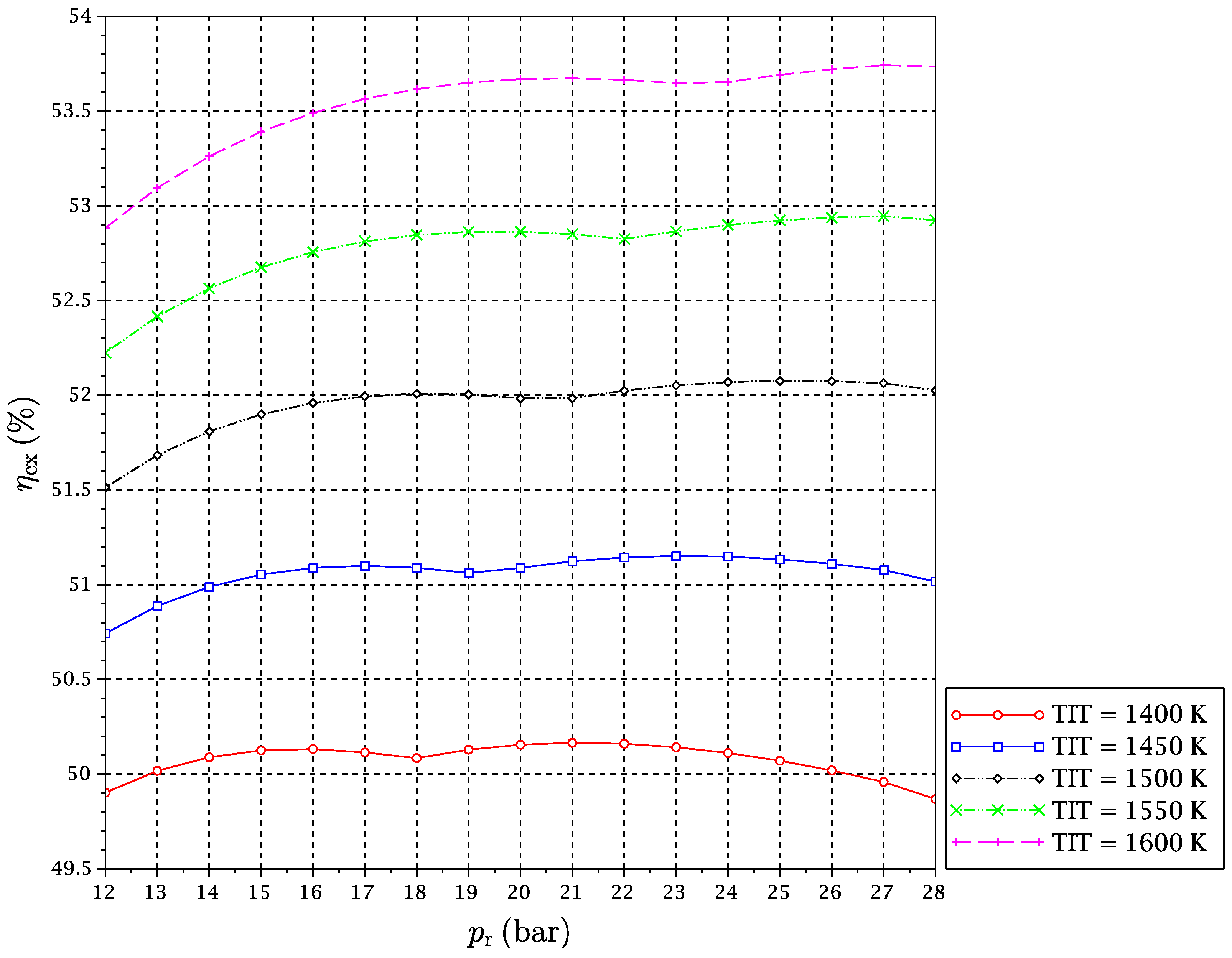
Figure 10). We will refer to this point of tendency change as the reduction reactor heating uncoupling point (RRHUP). This phenomenon is also revealed in the thermal efficiency plots. Instead of the usual curves with a maximum that are found for a conventional combined cycle, curves with two local maxima of quite similar values are obtained for this CLC system (
Figure 5,
Figure 6 and
Figure 7). Consequently, a good thermal efficiency that is almost constant is achieved along a quite wide range of pressure ratios.
Table 2 shows the position of the exergy efficiency maximum found for each TIT curve (the highest of both), together with the optimal reduction temperatures for these maxima.
It can be noticed that Syngas B presents a higher exergetic efficiency and lower reduction temperature than Syngas A. This is justified on the basis of the different hydrogen contents of both syngases. More hydrogen implies more need for heat at the reactors, and temperature must be lowered to satisfy the energy balance. In addition, the “chemical heat pump” effect leads to a higher exergy efficiency. Syngas C has an intermediate content of hydrogen, but also a significant extra amount of carbon monoxide. Since the oxidation of carbon monoxide is slightly exothermic, the reduction temperature can be increased a bit, and the exergy efficiency obtained is consequently the highest of the three fuels under study. Another interesting point is that for the case of Syngas B, the highest maximum is the left one, i.e., at lower , while for Syngases A and C, the highest maximum is the right one, i.e., at higher . In any case, the difference in the exergy efficiency between Syngases B and C is very slight.
The thermodynamic conditions of the whole optimized CLC cycle are fully given in
Table 3 for the case of Syngas C and TIT equal to 1550 K, as an example. The temperature, pressure and composition of all cycle points represented in
Figure 2 can be read from the table. Points 23–26 (not shown in
Figure 2) correspond to a conventional one pressure level steam cycle.
3.3. Exergy Balances
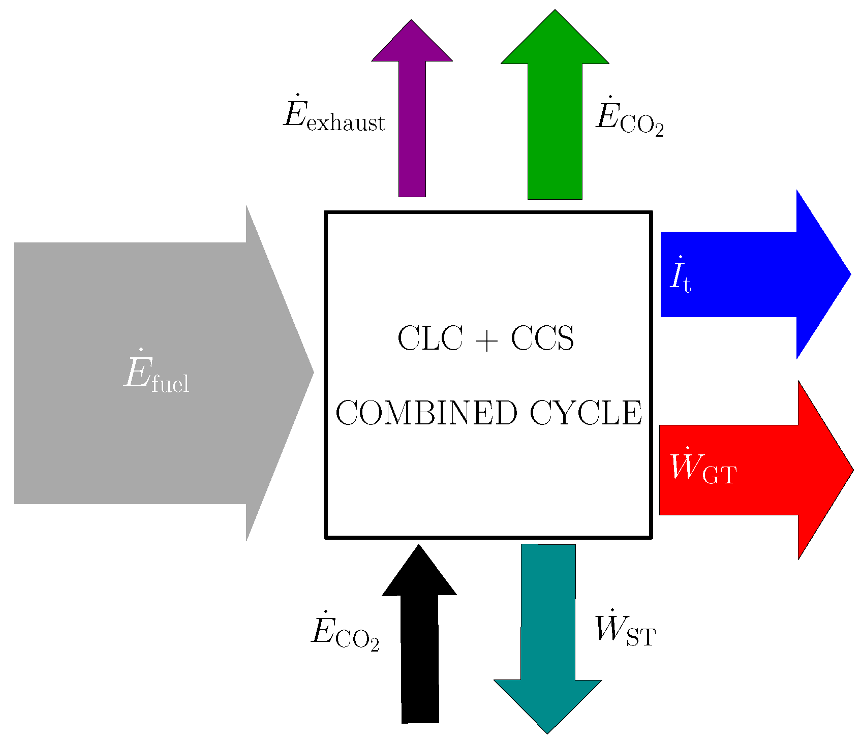
Figure 11 illustrates the exergy flows in the proposed CLC power plant. The exergy input to the power plant is fuel’s exergy, mainly the chemical exergy term, but also the physical exergy term. The exergy outputs are the compressed CO
2 stream and the flue air stream. The exergy content of the latest of both is as a matter of fact a non-recoverable exergy term, so it could be considered as an exergy loss somehow. Another part of the fuel’s exergy content is transformed to power in the gas turbine cycle and in the steam cycle. Some of this power must be reinjected to the cycle as the power consumption of CO
2 compressors. Finally, the rest of the fuel’s exergy content is lost, due to irreversibilities in the cycle and heat losses to the environment.
A quantification of the exergy distribution is shown in
Table 4 for a particular case with
, under the optimal conditions for each syngas, given in
Table 2. Values are given as a fraction of the exergy input to the cycle, i.e., normalized by
.
It may be of interest to remark on the influence of the CO
2 compression power consumption in the exergy efficiency of the cycle. The difference between Syngases A and C is about 1.4 percentage points, much more significant than the influence of power generation by gas turbines and steam turbines, and it would be higher if the storage pressure of CO
2 were increased. This term can be seen as approximately proportional to the carbon plus inert gases content of syngas (massflow to be compressed per mol of fuel) and approximately inversely proportional to the fuels chemical exergy. This could be characterized by a fuel dependent carbon and inert/exergy parameter:
that can be obtained from
Table 1 for the fuels under study:
and is more or less proportional to the
values given in
Table 4.
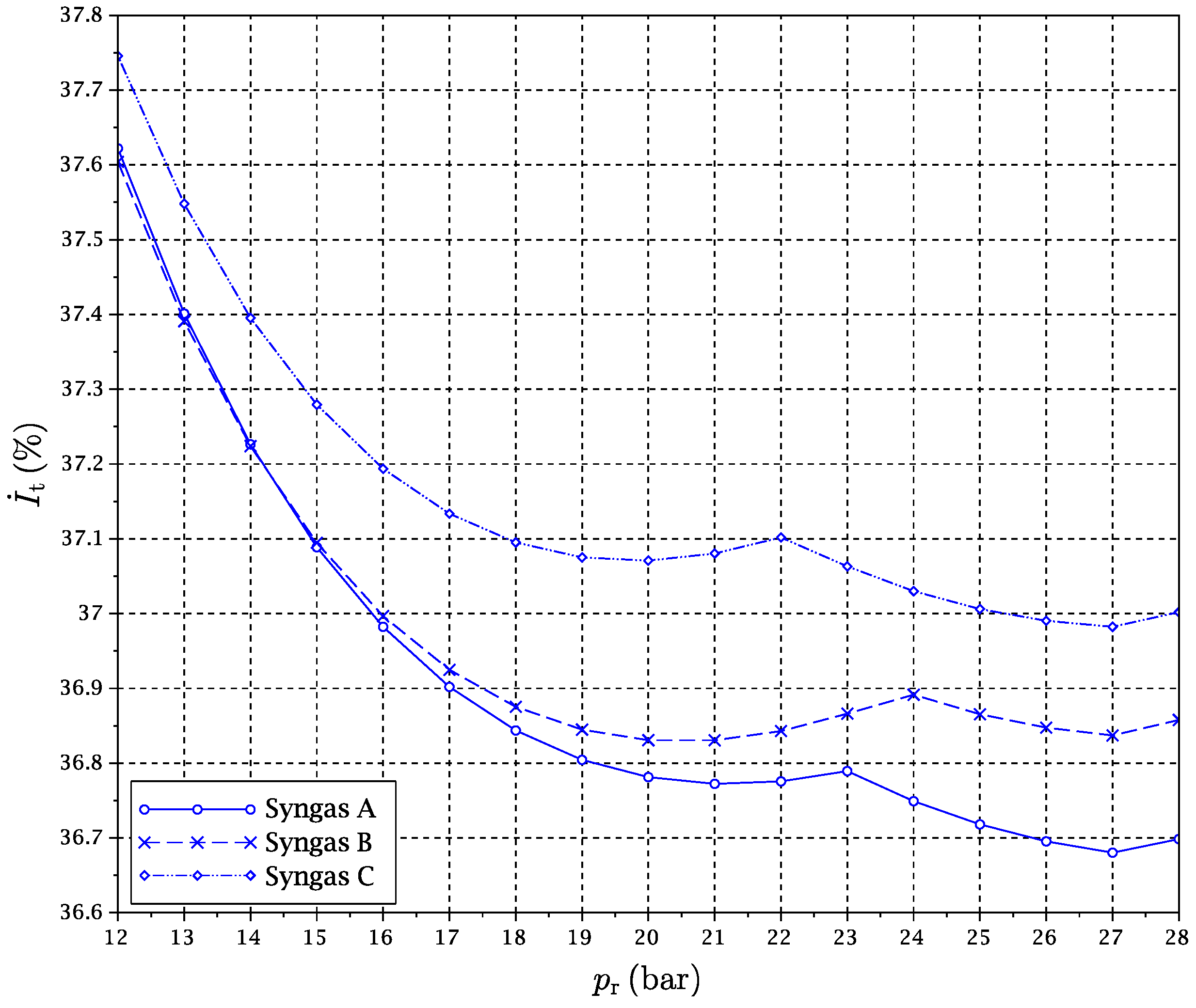
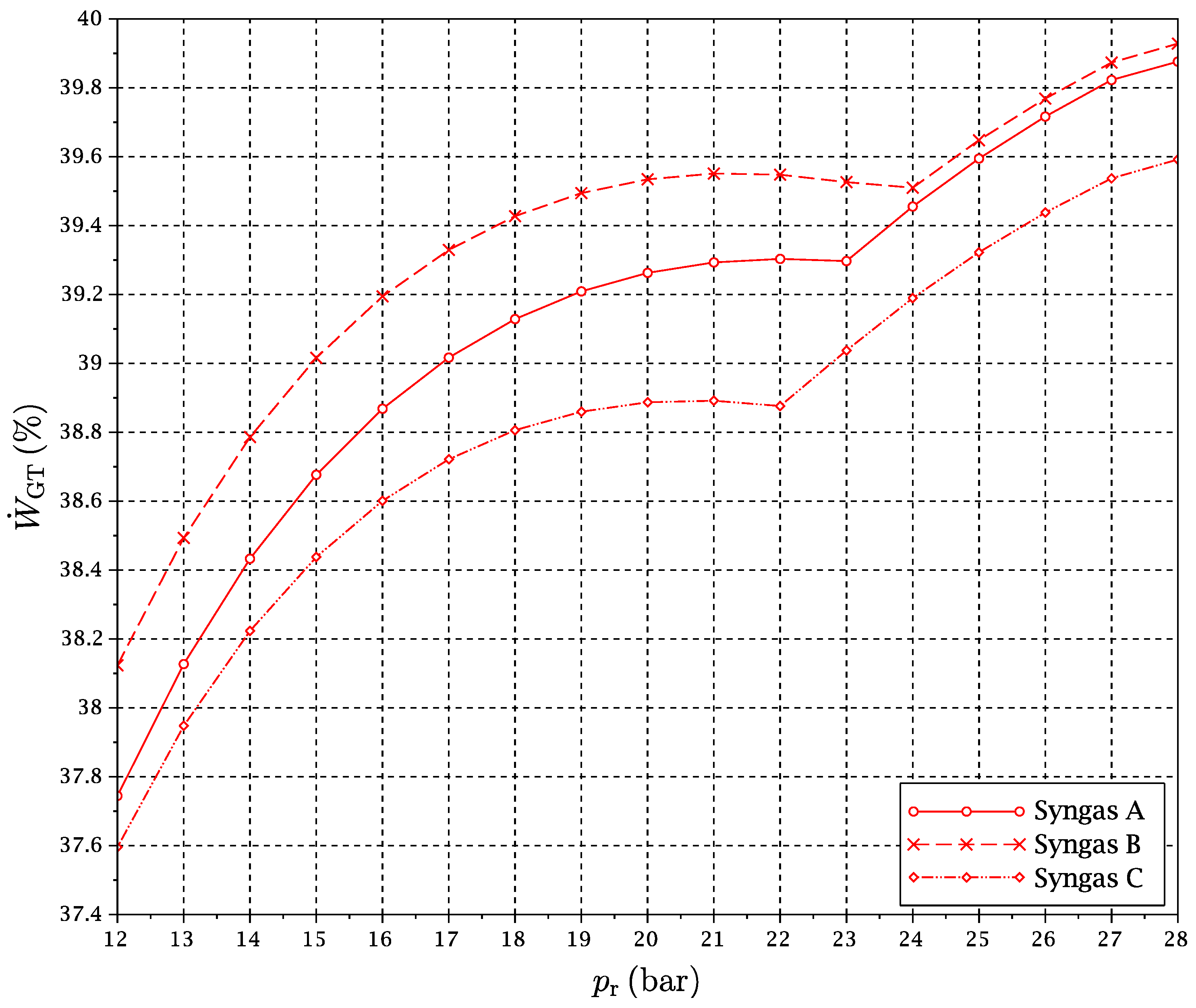
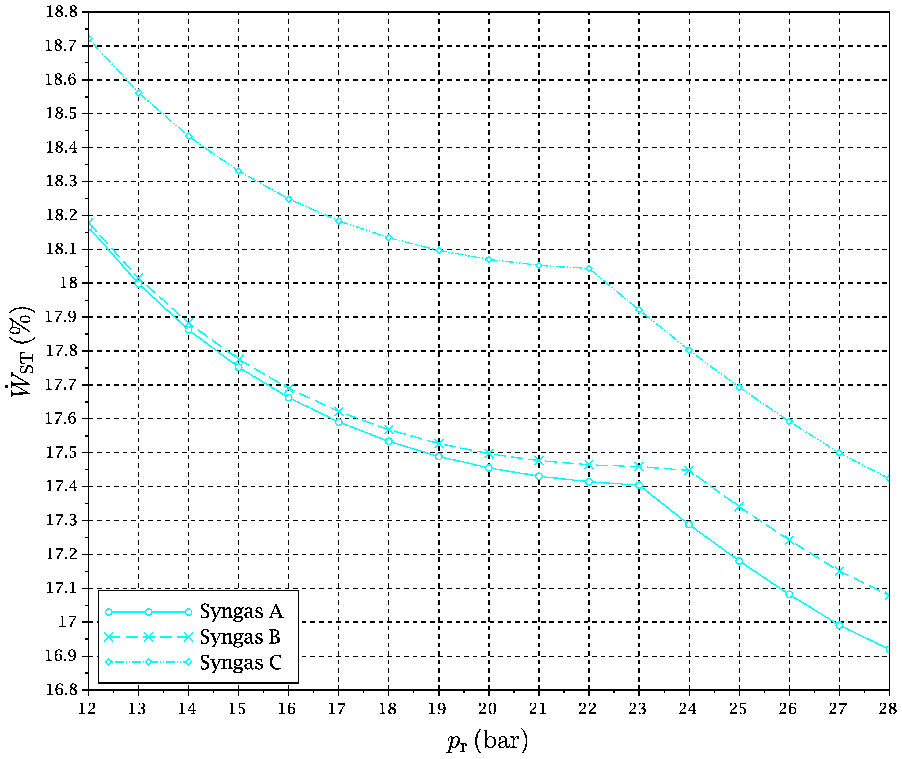
It is also interesting to analyze the dependence of the main exergy flows with the operating conditions. A negligible dependence is found for the exergy content of flue air, CO
2 compression power and stored CO
2 flow, since their conditions are more or less uncoupled from the rest of the cycle. The exergy flows of total exergy loss, gas turbines power production and steam turbine power production as a function of pressure ratio have been plotted in
Figure 12,
Figure 13 and
Figure 14 for a particular value of TIT. Values are given as a fraction of
.
All of
Figure 12,
Figure 13 and
Figure 14 show clearly the abrupt change of tendency associated with the RRHUP. In particular,
Figure 13 reproduces how an important extra amount of power is produced by GT1 when the reduction temperature begins to increase as the RRHUP is reached due to the combination of the “power heat pump” and “chemical heat pump” effects mentioned previously. This is partially compensated by the lower power produced by the steam cycle (
Figure 14), since the temperature of the air stream entering the HRSG decreases quickly with the pressure ratio. However, the combination of both effects and a low total exergy loss (
Figure 12), allows one to obtain a second maximum in the overall exergy efficiency in a zone of higher pressure ratios (see
Figure 5,
Figure 6 and
Figure 7).
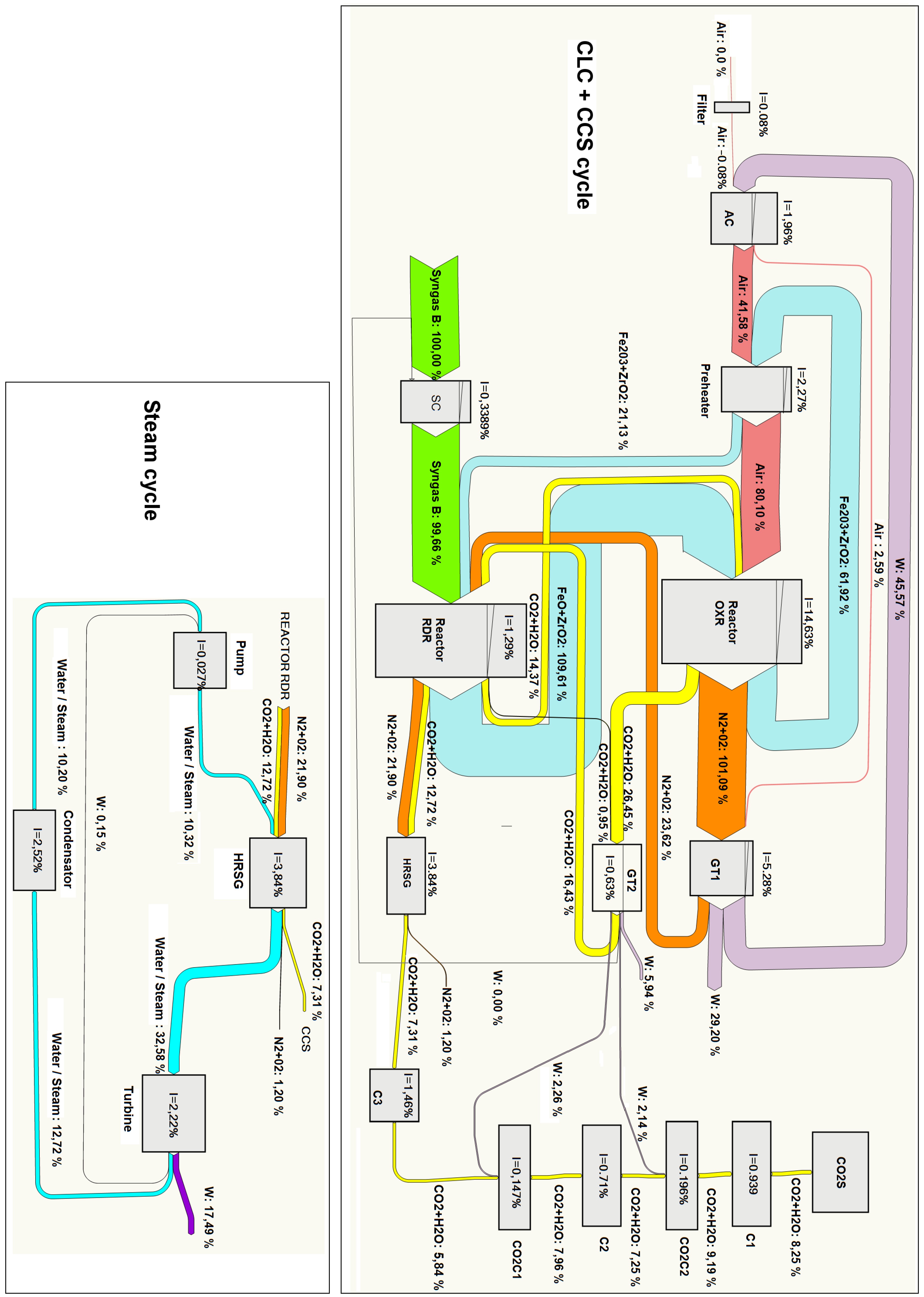
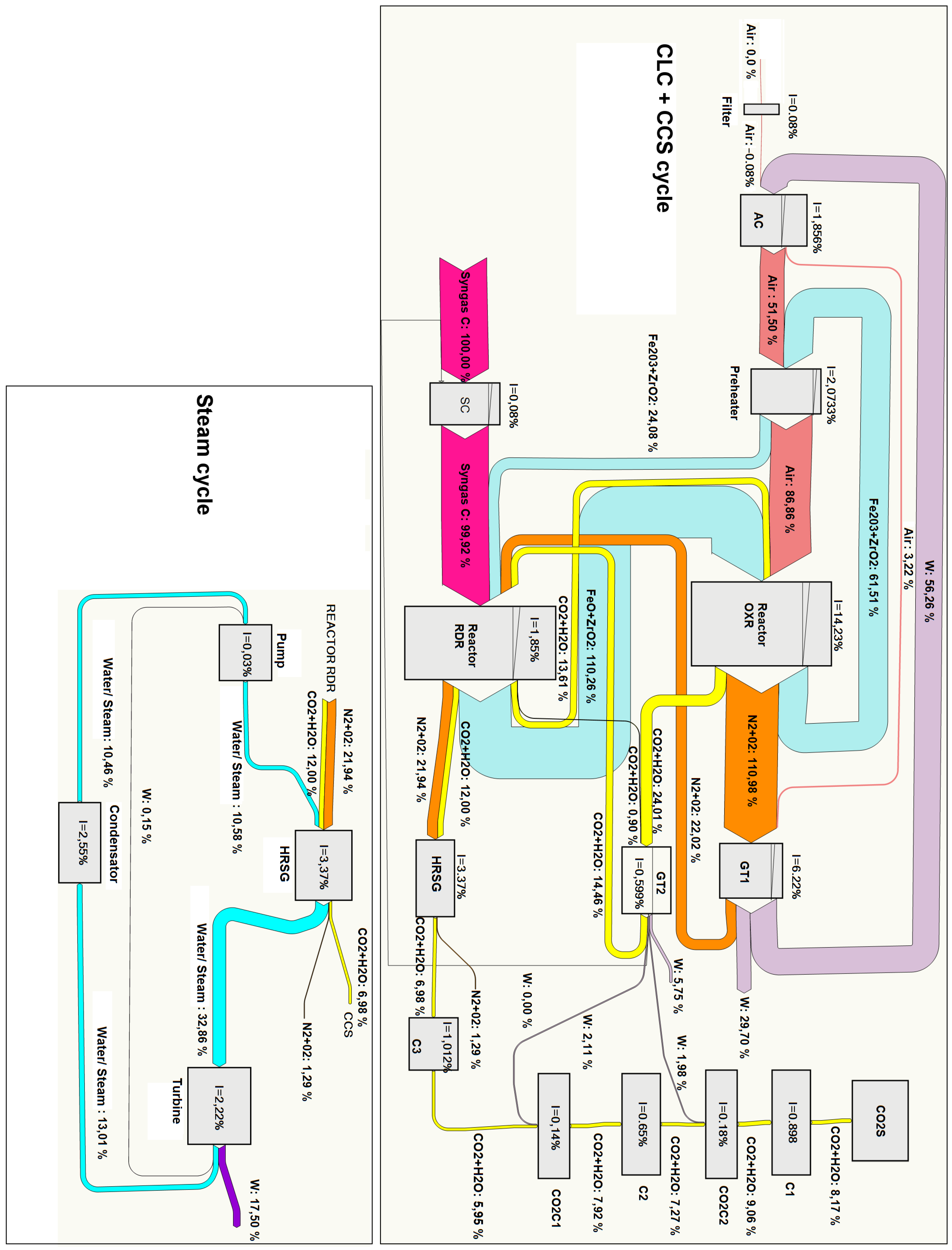
A more detailed exergy analysis is often presented in the form of a Grassmann diagram. This kind of chart reproduces the exergy flows associated with the different streams connecting the different components of the cycle. Furthermore, mechanical power input or output in every component is shown, and the exergy loss is indicated as a decrease in the exergy flow out of the component. In this way, the displayed graphical information allows one to identify easily the components with large exergy destruction. We present in
Figure 15 and
Figure 16 Grassmann diagrams for two cases: Syngas B and Syngas C under optimal conditions for
. With the aim of facilitating the interpretation of the figures, we remark that the exergy inputs are represented on the left side and the exergy outputs on the right side of each component.
The main differences between both cases can be summarized as follows:
The optimal pressure for Syngas B is and for Syngas C is . As mentioned previously, this is related to the fact that for Syngas B, the optimal point is reached at pressures lower than the RRHUP, and for Syngas C, the optimal point is found at higher pressures. This is reflected in higher compression power, higher flow exergy of air and oxygen carrier streams and higher power production in GT1 for the case of Syngas C.
The exergy destruction in the “syngas compressor” is very small for the case of Syngas C. Actually, since fuel admission pressure has been set at , as a matter of fact, the “syngas compressor” is acting merely as an isenthalpic pressure loss instead of a compression in both cases represented here. However, the pressure loss is very small for the case of Syngas C (down to ) and somewhat larger for Syngas B (down to ).
For the steam cycle block and the CO2 sequestration module, the results are very close to each other.
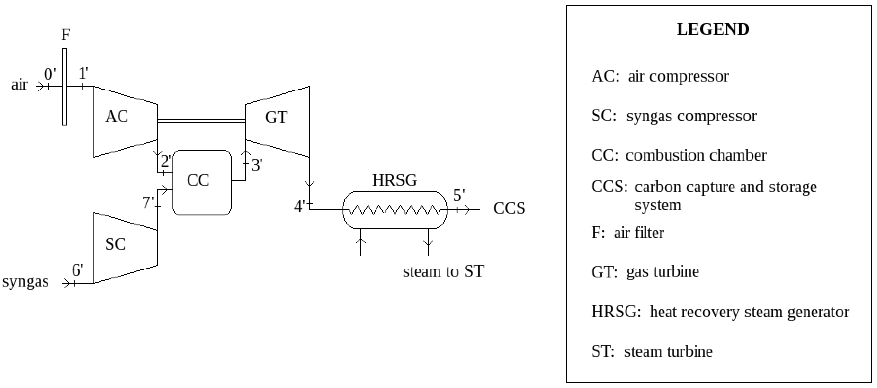
3.4. Comparison with a Conventional Gas Turbine Cycle
In order to illustrate the important differences regarding the exergetic behavior between a CLC gas turbine system and a conventional gas turbine system, we have carried out a comparison of the exergy flows of this part of the cycle.
Table 5 compares the following exergy flows for a reference case of
and
: the exergy flow of the exhaust gases stream before entering the HRSG, the power generated by the gas turbine block, the exergy loss in the combustion chamber and the exergy losses in the rest of the cycle, all of them given as a fraction of the fuels exergy.
Figure 17 gives further details of the evolution of the total exergy destruction involved in combustion with the compression pressure ratio, both via CLC and conventional combustion, for
.
It can be noticed that the exergy destruction in the combustion chamber is of the order of five percentage points lower for the CLC cycle. This quantifies the “chemical heat pump” effect in terms of exergy savings. On the other hand, the additional heat and pressure losses and the exergy destruction in heat exchangers involved in the CLC case make the total exergy losses more similar when the whole gas turbine system is considered. Still, the overall exergy loss is lower and the power generated is slightly higher for the CLC cycle. In addition, more exergy is carried by the stream entering the HRSG, expecting a little more of the power to be obtained by the steam cycle. This point can be surprising at first sight, since some heat must be taken from the gas streams outgoing from the turbines in the case of the CLC system. Nevertheless, it must be kept in mind that the expansion in GT2 is carried out down to a pressure of
(for optimization purposes, when CO
2 compression takes part; see
Section 3.2) instead of to approximately the atmospheric pressure, as happens in a conventional gas turbine. Thus, the temperature of this stream is increased in relation to the conventional gas turbine. As a result, the power produced by the ensemble is a little bit larger for the CLC gas turbine system.


