Figure 1.
(log-log plot). For the case with (blue curve) and, for the case , the crossover between two curves, namely with (black curve) and (red curve) respectively, both with . For the red curve, we have the crossover characteristic values , which indicate the passage from one regime to another.
Figure 1.
(log-log plot). For the case with (blue curve) and, for the case , the crossover between two curves, namely with (black curve) and (red curve) respectively, both with . For the red curve, we have the crossover characteristic values , which indicate the passage from one regime to another.
Figure 2.
Crossovers in for (log-log plots) (a) between two curves with (red curve), (blue curve) respectively, both with ,,1), and (b) a change was done on the blue curve, with (black curve); the cutoff occurs at .
Figure 2.
Crossovers in for (log-log plots) (a) between two curves with (red curve), (blue curve) respectively, both with ,,1), and (b) a change was done on the blue curve, with (black curve); the cutoff occurs at .
Figure 3.
(log-log plot) of three curves (case ) with parameters and (blue dashed curve), (red dashed curve), and their linear combination (black curve) with and .
Figure 3.
(log-log plot) of three curves (case ) with parameters and (blue dashed curve), (red dashed curve), and their linear combination (black curve) with and .
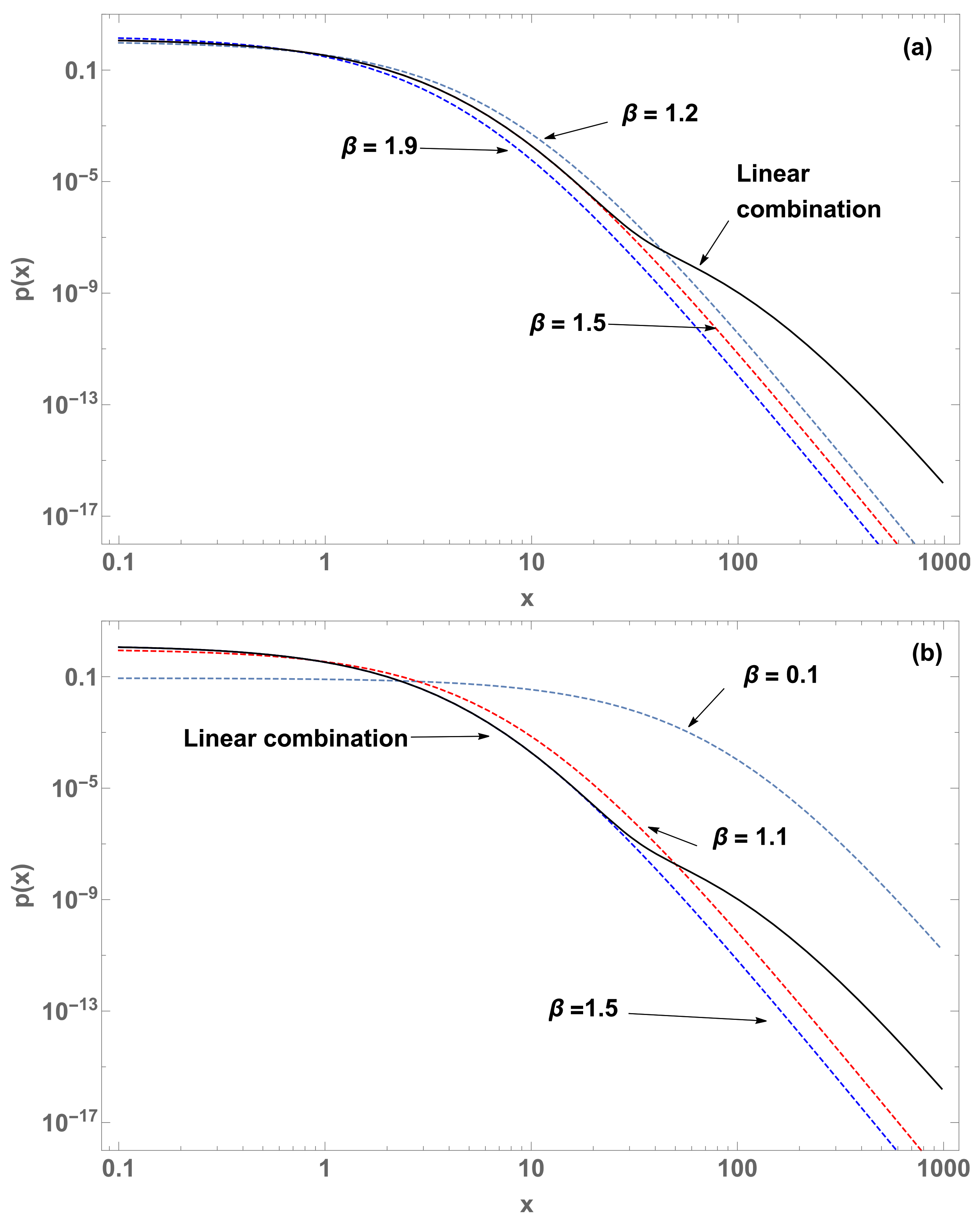
Figure 4.
(log-log plots) of four curves with parameters , (blue dashed curve), (red dashed curve), (gray dashed curve), and their linear combination (black curve). (a) Four curves with (blue dashed curve), (red dashed curve), (gray dashed curve) and their linear combination (black curve). (b) With , and , both with (case ).
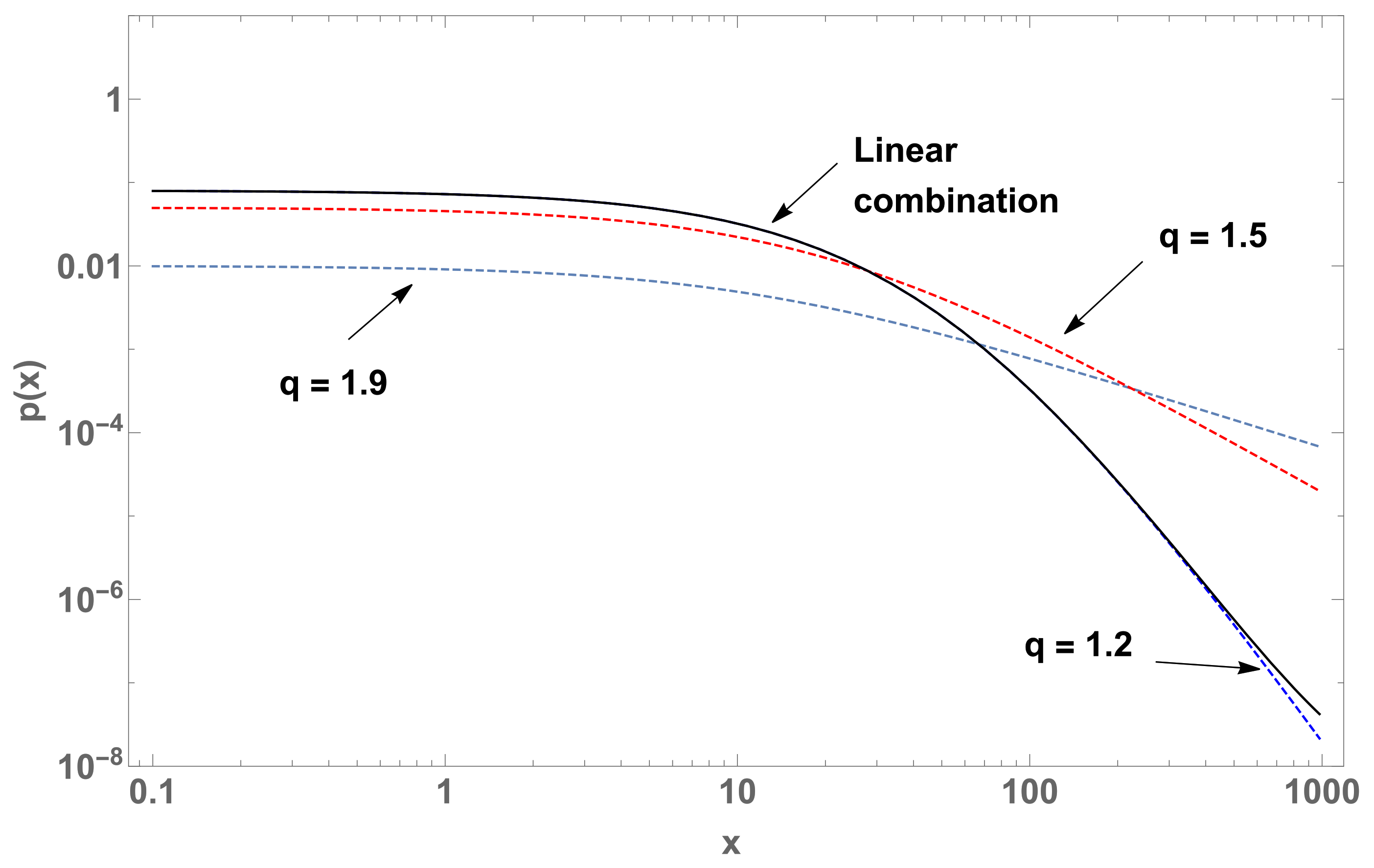
Figure 5.
(log-log plot) of four curves (case ) with parameters , (blue dashed curve), (red dashed curve), (gray dashed curve), and their linear combination (black curve) with , and .
Figure 5.
(log-log plot) of four curves (case ) with parameters , (blue dashed curve), (red dashed curve), (gray dashed curve), and their linear combination (black curve) with , and .
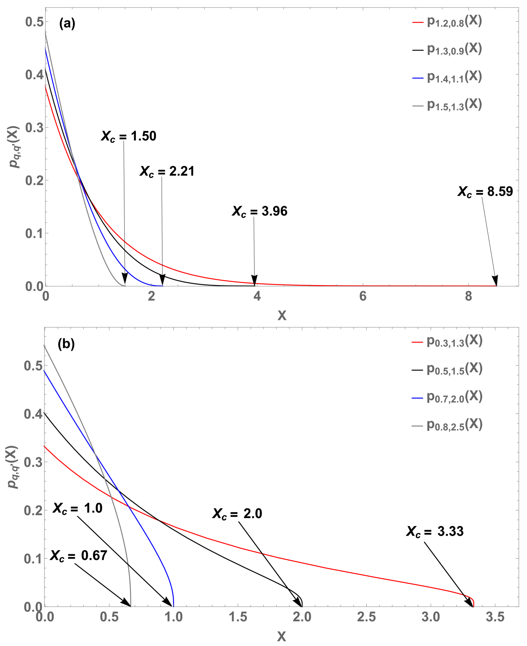
Figure 6.
Four probability distributions
(
M = 3) based on Equation (
30) with
. From (
31), we respectively obtain the cutoff values
for
(blue curve),
for
(black curve),
for
(gray curve) and
for
.
Figure 6.
Four probability distributions
(
M = 3) based on Equation (
30) with
. From (
31), we respectively obtain the cutoff values
for
(blue curve),
for
(black curve),
for
(gray curve) and
for
.
Figure 7.
Three probability distributions
based on Equation (
33) with
and
hence
(black curve),
hence
(red curve), and
hence
(blue curve).
Figure 7.
Three probability distributions
based on Equation (
33) with
and
hence
(black curve),
hence
(red curve), and
hence
(blue curve).
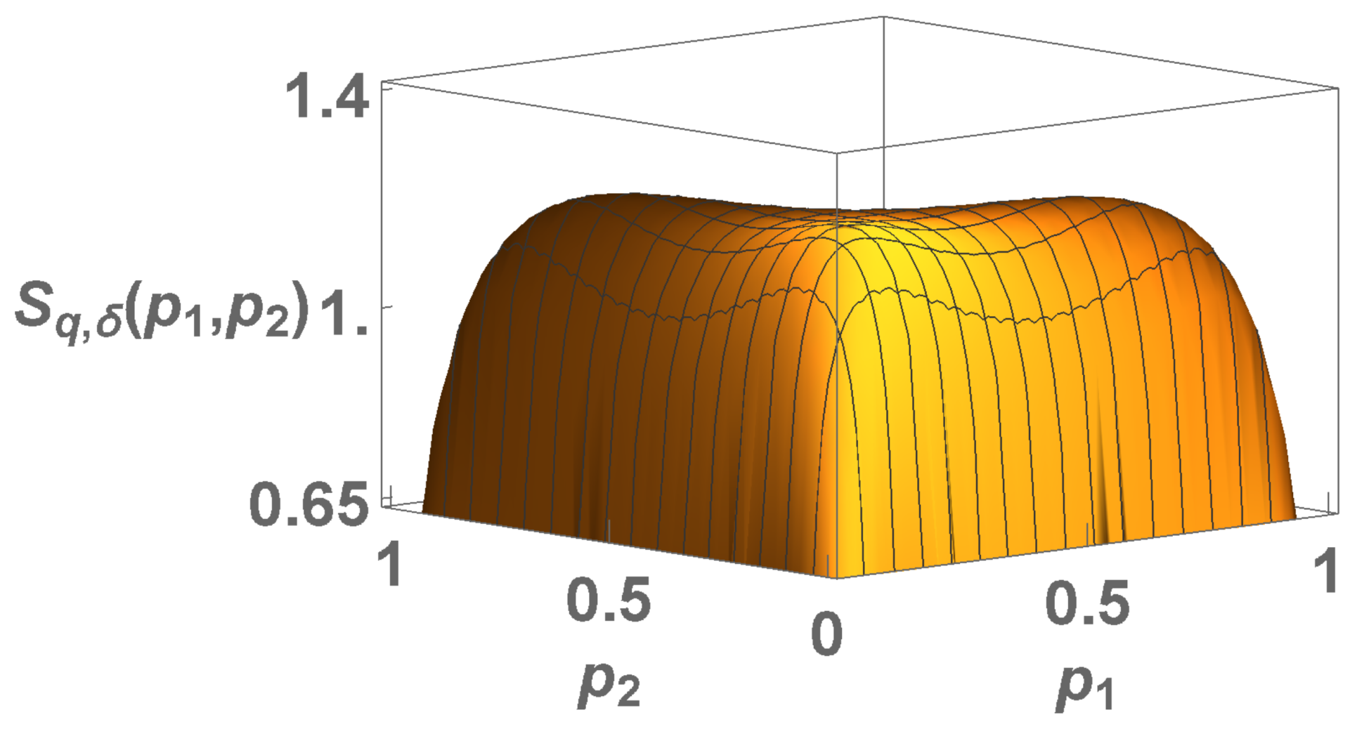
Figure 8.
Concavity/convexity mapping for (
41) with
,
(
a) and
(
b). The green (pink) region represents all points whose entropy (
41) is concave (convex). The black region represents all points whose entropy is neither concave nor convex, having two local minima points and a local maximum in between (a global maximum point at
and divergences at
and
). On the red point is localized the Boltzmann–Gibbs entropy and over the red dashed line cutting the origin, we have all the
entropies. On the concave (convex) region we have
(
). (
c) Four (
) entropies with
, and
(blue curve),
(green curve),
(black curve) and
(pink curve).
Figure 9.
Illustrative probability distributions
. (
a)
and
hence, through (
45),
(gray curve);
, hence
(black curve);
hence
(red curve) and finally,
hence
(blue curve); (
b)
hence
(blue curve);
hence
(red curve);
hence
(black curve); and
hence
(gray curve).
Figure 9.
Illustrative probability distributions
. (
a)
and
hence, through (
45),
(gray curve);
, hence
(black curve);
hence
(red curve) and finally,
hence
(blue curve); (
b)
hence
(blue curve);
hence
(red curve);
hence
(black curve); and
hence
(gray curve).
Figure 10.
Concavity/convexity regions for
(
46) (
a)
. (
b)
. The green (pink) region represents all points whose entropy (
41) is concave (convex). The black region represents all points whose entropy is neither concave nor convex, having two local maxima ( inflexion) points and another local minimum (maximum) in between. The points of transition at
are:
(both
and
) (
);
(
) and
(
) (
) and
(both cases) (
). At
, we have the transition from non concave to concave at
(
) and for
, we have
. The blue dashed horizontal line represents
, while the red dashed vertical line represents all
entropies, and the red point is the BG entropy. (
c) Four cases (
) for
with the respective colors:
and
(convex and concave regions respectively);
(black region) and
(purple region) (non concave and non convex regions).

Figure 11.
Plot for with , and . We clearly observe that is not valid here, because in this value, the entropy is not concave, much less the values close to this.
Figure 11.
Plot for with , and . We clearly observe that is not valid here, because in this value, the entropy is not concave, much less the values close to this.
Figure 12.
Plot for with . Here, . In the inset, we indicate the behavior of that function closer to origin.
Figure 12.
Plot for with . Here, . In the inset, we indicate the behavior of that function closer to origin.
Figure 13.
Plot for with . The regression by excluding the and points yields an 8th degree polynomial of , namely . It means that, when we have , thus , therefore which diverges at infinity.
Figure 13.
Plot for with . The regression by excluding the and points yields an 8th degree polynomial of , namely . It means that, when we have , thus , therefore which diverges at infinity.
Figure 14.
Eight illustrative Borges–Roditi probability distributions. (a) (red curve); (black curve); (blue curve), and (gray curve). (b) (red curve), (black curve), (blue curve), and (gray curve).
Figure 14.
Eight illustrative Borges–Roditi probability distributions. (a) (red curve); (black curve); (blue curve), and (gray curve). (b) (red curve), (black curve), (blue curve), and (gray curve).
Figure 15.
Concavity/convexity for
(
49) with (
a)
and (
b)
. The green (pink) region represents all points whose entropy (
49) is concave (convex). The black (purple) region represents all points whose entropy is neither concave nor convex, having two local maxima (inflexion) points and another local minimum (maximum) in between. The red dashed vertical lines represent all
entropies and the red point is the BG entropy, while the light (dark) blue lines represents all Shafee
(Kaniadakis
) entropies [
29,
30]. (
c) Four illustrative cases (
) with
and its respective colors:
and
(pink and green regions respectively );
(black region) and
(purple region).
Figure 16.
Eight illustrative probability distributions . (a) (gray curve), (blue curve), (black curve), and (red curve). (b) (gray curve), (blue curve), (black curve), and (red curve).
Figure 16.
Eight illustrative probability distributions . (a) (gray curve), (blue curve), (black curve), and (red curve). (b) (gray curve), (blue curve), (black curve), and (red curve).
Figure 17.
Concavity/convexity for
(
55) with (
a)
and (
b)
. The green (pink) region represents all points whose entropy (
55) is concave (convex). The black (purple) region represents all points whose entropy is neither concave nor convex, having two local maxima (inflexion) points and another local minimum (maximum) in between. The red dashed vertical line represents all
entropies and the red point is the BG entropy. (
c) Four cases (
) with the respective colors: with
,
and
(pink and green regions) and
(black region), and
(purple region).


