Abstract
This paper introduces a direct method derived from the global radial basis function (RBF) interpolation over arbitrary collocation nodes occurring in variational problems involving functionals that depend on functions of a number of independent variables. This technique parameterizes solutions with an arbitrary RBF and transforms the two-dimensional variational problem (2DVP) into a constrained optimization problem via arbitrary collocation nodes. The advantage of this method lies in its flexibility in selecting between different RBFs for the interpolation and parameterizing a wide range of arbitrary nodal points. Arbitrary collocation points for the center of the RBFs are applied in order to reduce the constrained variation problem into one of a constrained optimization. The Lagrange multiplier technique is used to transform the optimization problem into an algebraic equation system. Three numerical examples indicate the high efficiency and accuracy of the proposed technique.
1. Introduction
The purpose of the calculus of variations is to find functionals achieving the extremal (maximum or minimum) value. The direct approaches convert the variational problems (VPs) into a mathematical programming problem. Schechter [1] adopted the direct scheme of Galerkin and Ritz to approximate VPs. The authors of [2,3,4,5,6,7] introduced the Walsh series method, Legendre wavelets technique, Legendre polynomials, Laguerre polynomials, Chebyshev series and differential transformation method, respectively. Yousefi and Dehghan [8] applied the He’s variational iteration technique to simulate variational problems. Recently, Golbabai and Saeedi [9] used a meshless method to approximate VPs arising from a dynamic investment model.
In this paper, we introduce a numerical approach for approximating the two-dimensional variational problem (2DVP) for functionals depending on the function of several independent variables in the following form:
in which x and y are the independent variables of which is a continuous function with continuous partial derivatives with respect to x and y, respectively. The symbol represents the area of the fixed region in the x–y plane.
In this work, we introduce the radial basis function (RBF) collocation method to simulate 2DVPs for functionals depending on the function of several independent variables. The presented strategy parameterizes the solutions with arbitrary global RBFs (GRBFs) and transforms the 2DVP into a constrained optimization problem by means of arbitrary collocation nodes. One may select the interpolation function from the family of GRBFs, such as the multiquadric (MQ), Gaussian (GA), inverse multiquadric (IMQ), etc., functions. A major benefit of the RBF method is its arbitrary discretization. The proposed technique does not require a node grid for discretizing and provides a higher level of flexibility in selecting the collocation points. By means of the Legendre–Gauss–Lobatto (LGL) quadrature and the method of Lagrange multipliers, the problem is reduced to an algebraic equation system. After solving the algebraic equations, the unknown coefficients can be obtained.
The layout of the current paper is organized as follows: Section 2 introduces some properties of RBFs. Section 3 uses the RBF collocation method to solve variational problems for functionals depending on the function of several independent variables. Section 4 presents three numerical examples illustrating the accuracy of the RBF collocation method. Finally, Section 5 contains the concluding remarks.
2. Properties of RBFs
RBFs are very powerful mathematical tools and deserve special attention in the field of computational science. Hardy [10] first introduced the RBFs interpolation to approximate two-dimensional geographical surfaces based on scattered data. Later, Kansa [11,12] first adopted the MQ-RBF collocation technique to approximate PDEs of parabolic, elliptic and hyperbolic types. Recently, Golbabai et al. [13,14] used an RBF collocation technique for a nonlinear models. The meshfree RBF method is used in both local and global forms. Some authors have tried localized-RBF-based strategies, such as the localized-RBF-generated FD (RBF-FD) [15,16,17,18,19,20,21,22,23,24] and the RBF partition of unity (RBF-PU) [25,26,27,28,29,30,31,32,33,34,35].
Let be a given set of distinct centers. The approximation of a function using RBFs may be written as a linear combination
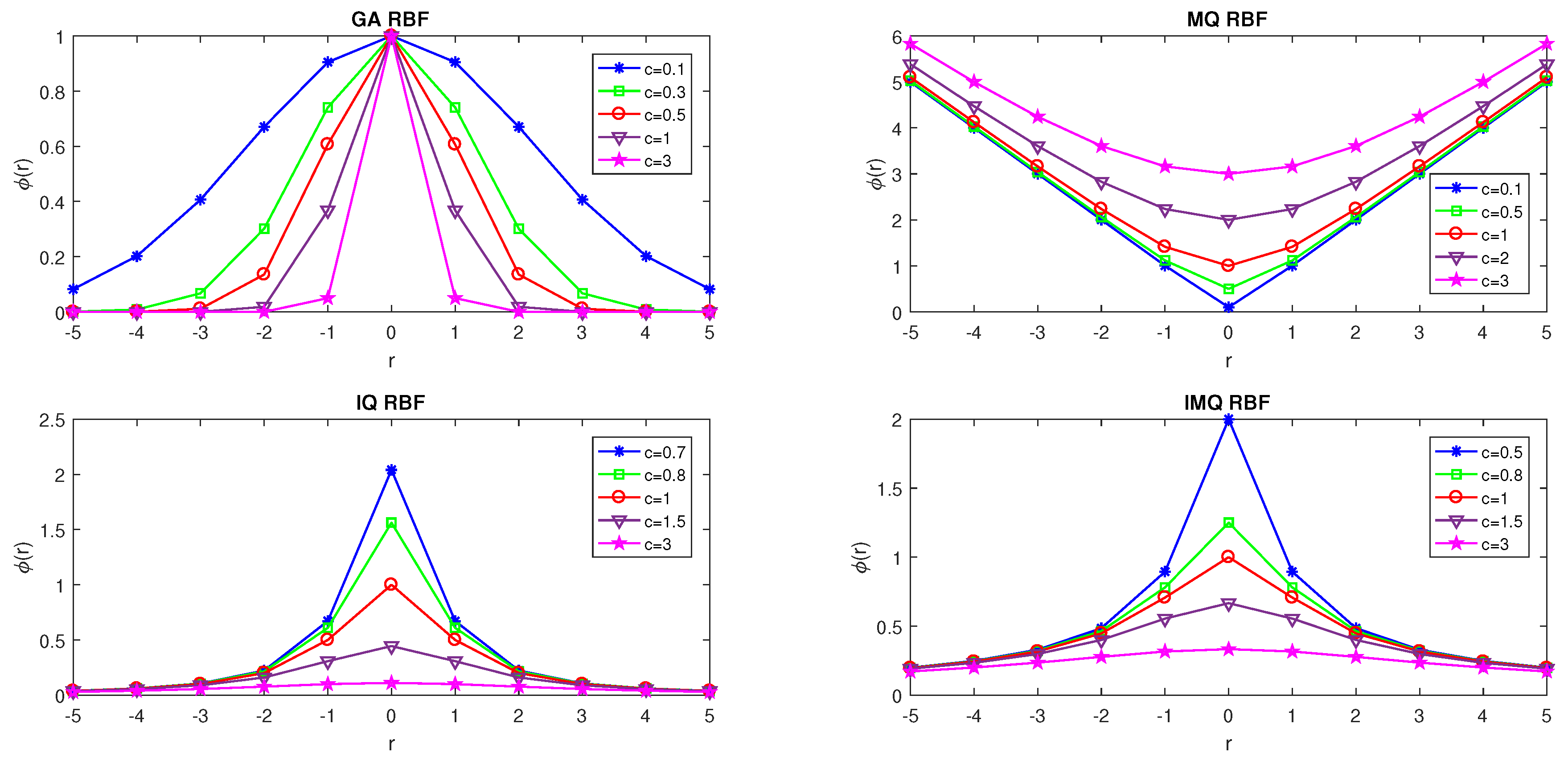
in which , are centers and are unknown coefficients for . Table 1 and Figure 1 illustrate some RBFs mathematically and graphically, respectively, where and denote the Euclidean norm and c is a positive shape (SP) which controls the width (flatness) of the basis function.

Table 1.
Mathematical form of some RBFs, ).
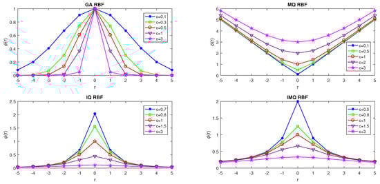
Figure 1.
Illustration of some RBFs.
Suppose that is a finite set of distinct nodal points. The unknown coefficients are determined so that for , which results in the linear system as follows
where the entries of the matrix are [36,37]. Since we choose to have global support, this method causes a dense matrix . The matrix has been proven to be positive definite for distinct interpolation nodes. Micchelli [38] proved that the matrix was positive definite for GA, IMQ and TPS RBF and conditionally positive definite for the MQ RBF method.
2.1. SP Strategies
The selection of the SP has a considerable effect on the stability and accuracy of an RBF method. There are different methods to select SPs. The most common are computing errors with distinct SPs and selecting the best one. SPs are categorized into two classes: constant and variable SPs.
2.1.1. Constant SPs
Constant SPs can be considered by Hardy and Franke’s formulas as follows:
- Hardy’s SP [10]in which N and represent the total number of centers and the distance from the ith center to the nearest neighbor, respectively.
- Franke’s SP [39]in which N and D denote the total number of centers and the diameter of the smallest circle encompassing all the center locations, respectively.
2.1.2. Variable SPs
A variable SP approach utilizes a different SP value at every center. This facilitates obtaining a different entry in the RBF matrices, leading to a lower condition number. Here, we list a number of variable SPs:
- Exponentially SP (ESP) [11]
- Sinusoidal SP (SSP) [40]
- Linear SP (LSP) [12]
- Random SP (RSP) [41]where and represent the maximum and minimum of ’s, respectively.
3. Numerical Solution of the Model
This section uses the RBF collocation technique to simulate variational problems for functionals depending on a function of several independent variables based on interpolating (GRBFs) over arbitrary collocation nodes. Let us find the extremal values of the following functional,
with the given boundary conditions (BCs) of the form
In order to provide a framework with a higher flexibility, different groups of collocation points, containing nodes with equal and unequal spacing, could be arbitrarily selected for the discretization. For instance, a set of Chebyshev–Gauss (CG), Gauss–Legendre (GL), Gauss–Lobatto (GLO), Gauss–Laguerre (GLA), Legendre–Gauss–Lobatto (LGL) and Chebyshev–Gauss–Lobatto (CGL) points can be chosen as a set of unequally spaced orthogonal points to approximate the desired model [42,43]. Now, we consider the following 2DVP for functionals depending on the function of several independent variables of Equations (9) and (10). The solution is approximated using RBFs as
where denotes the RBF interpolation of . Furthermore, denotes an RBF and represent the RBF weights related to .
Theorem 1.
Let and , then there exist partial derivatives with respect to x and y as follows:
Proof.
According to the definition of RBFs, , then the chain rule implies
Now, we obtain the partial derivative of with respect to x,
Subsequently, we can obtain the partial derivative of with respect to y. □
Theorem 2.
Let and , then there exist partial derivatives with respect to x and y as follows:
Proof.
According to the definition of RBFs, . Then, the chain rule implies
Now, we obtain the partial derivative of with respect to x,
Correspondingly, we can achieve the partial derivative of with respect to y. □
Now, by substituting Equation (11) and the partial derivatives obtained from Theorem 1 or Theorem 2 in Equations (9) and (10), we have
By applying LGL quadrature, we can approximate Equation (16) as follows,
in which and , denote the nodes LGL and , represent the LGL weights associated with LGL nodes , described as
in which denotes a Legendre polynomial of degree [44] and represent the RBF centers.
Finally, the constrained variational problem for functionals depending on the function of several independent variables of Equations (9) and (10) reduces to a constrained optimization problem
subject to
To solve the optimization problem of Equations (19) and (20), we adopt a Lagrange multipliers scheme and transform the problem into the following unconstrained optimization problem, so that,
where is the Lagrange multiplier related to the BCs. The unknown coefficients can be determined after solving the system as follows:
4. Numerical Experiments
This section considers three 2DVPs involving functionals that depend on functions of more than one independent variable to demonstrate the effectiveness of the presented technique. The numerical results indicate the advantages of this approach over the upwind technique, variational iteration scheme and other numerical techniques. In three test problems, different values of the SP and the data centers including uniform and Chebyshev nodes were adopted to show the advantage of the proposed strategy. For this aim, we defined the and norm errors to assess the efficiency and accuracy as:
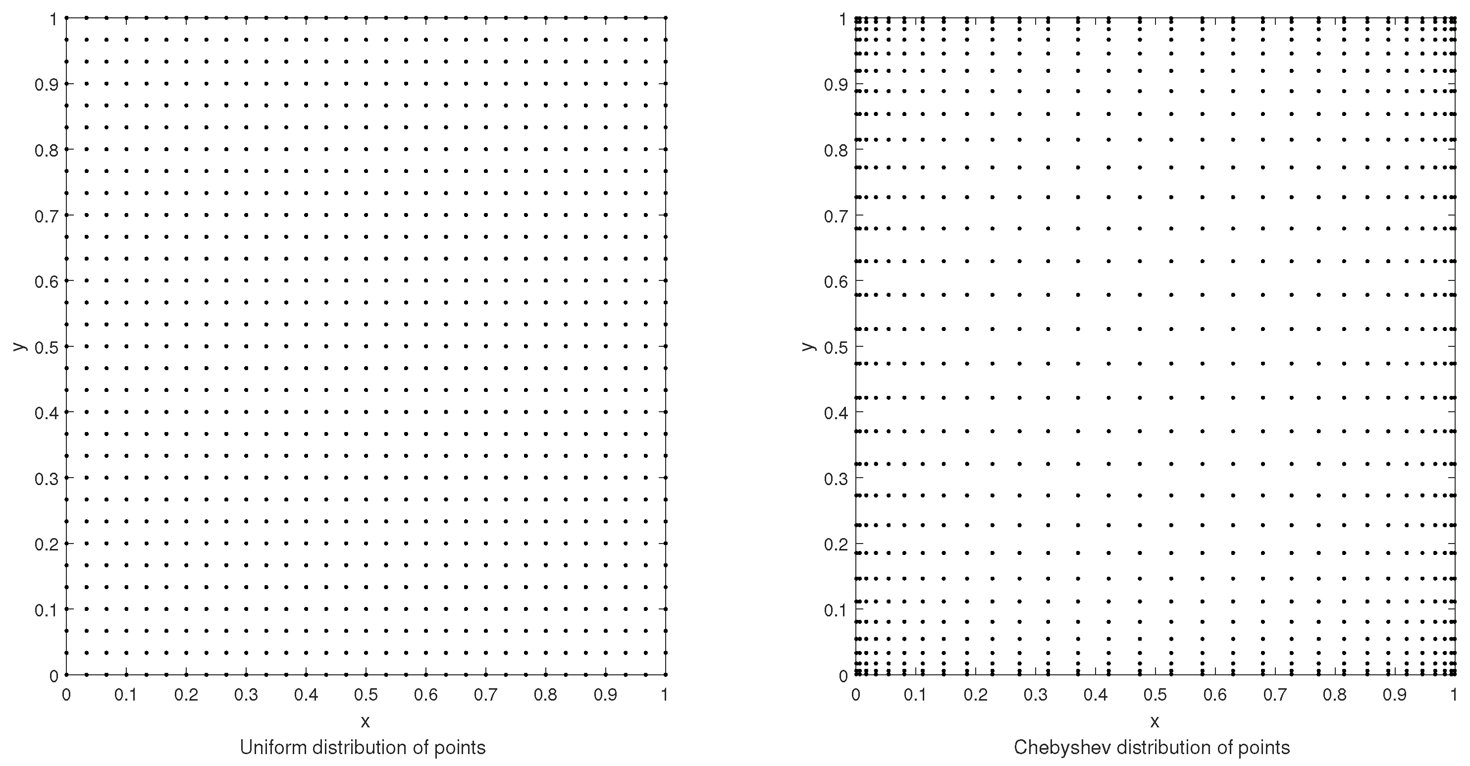
where and represent the exact and approximate solutions, respectively. Figure 2 shows the uniformly distributed and Chebyshev nodes. All numerical simulations were done by using MATLAB R2013b on a computer system having a configuration with 4.00 GB of RAM.
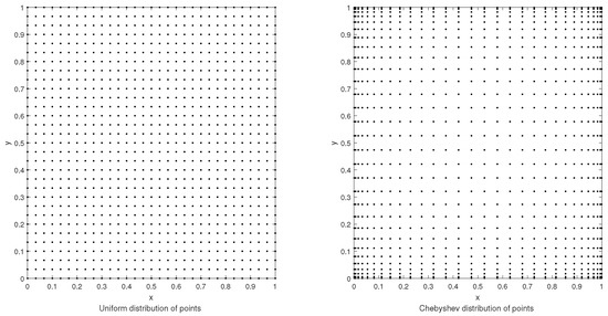
Figure 2.
Illustration of the uniformly distributed and Chebyshev nodes.
Example 1.
Let us consider the following 2DVP of finding the extremal of the functional
with the BCs
The exact solution of this problem is .
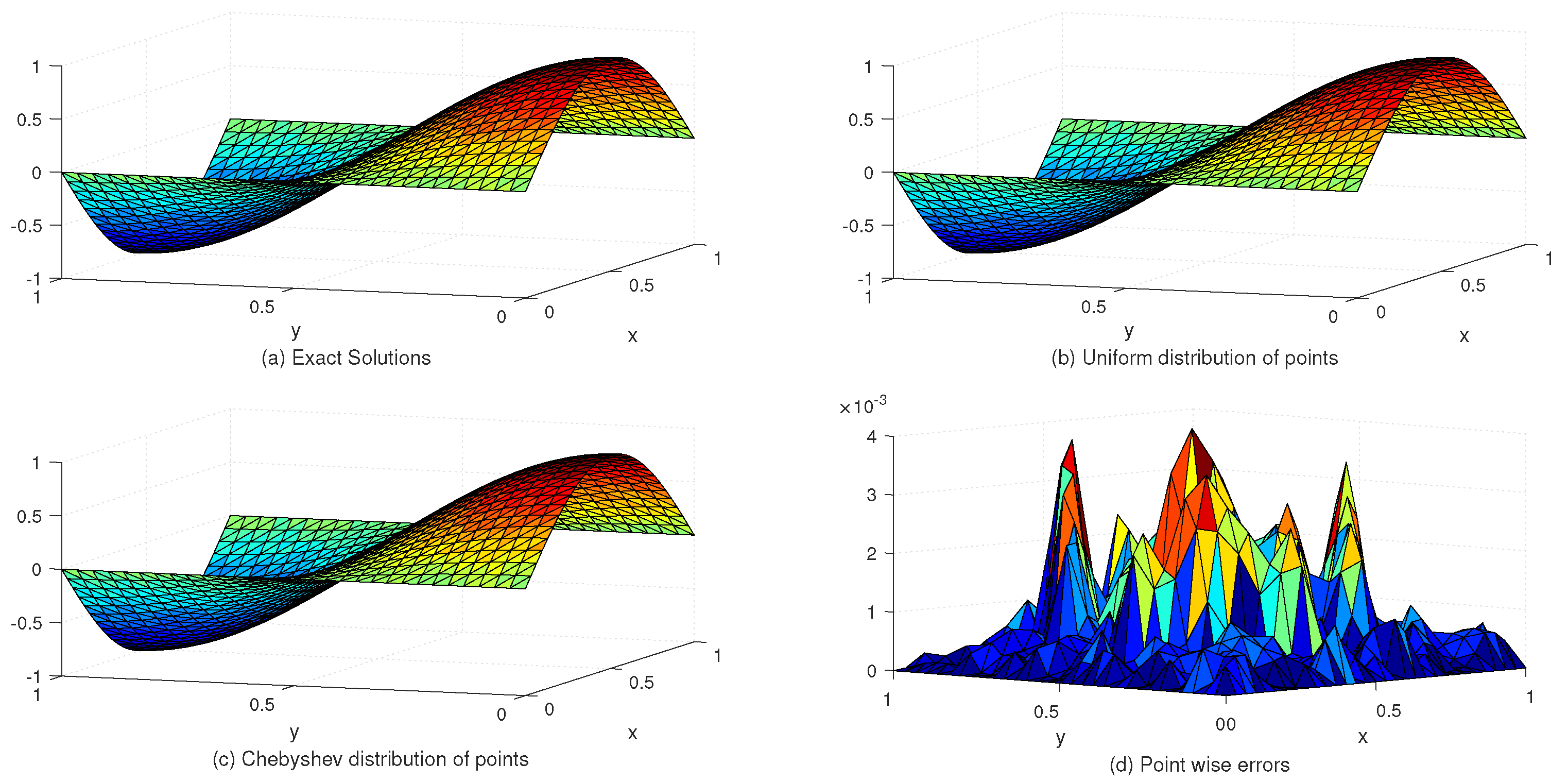
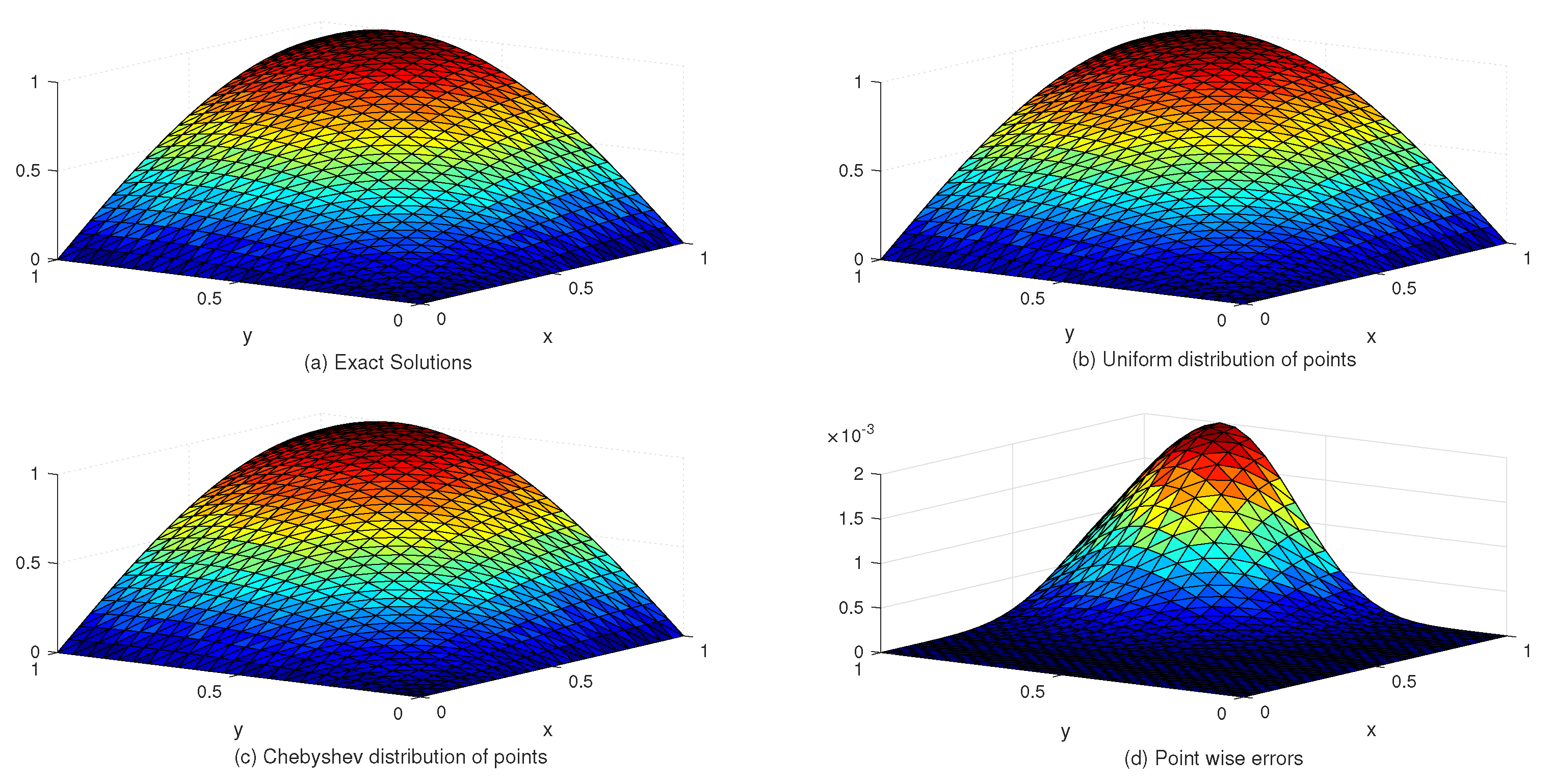
Table 2 lists the and error norms for several values of c with the uniform and Chebyshev nodes. In view of Table 2, we see that the accuracy of the numerical solution for uniform nodes is significantly better than that for Chebyshev nodes. Moreover, Table 3 shows the exact and approximate values of based on the proposed method. Figure 3 displays the exact and approximate solutions as well as the numerical errors with uniform and Chebyshev nodes at and . Finally, Figure 4 represents the behavior of the numerical errors for constant and variable SPs.
Table 2.
The and error norms for several values of c with the uniform and Chebyshev nodes in Example (1).
Table 3.
The approximate and exact values of .

Figure 3.
The behavior of exact and approximate solutions as well as numerical errors with and in Example 1.
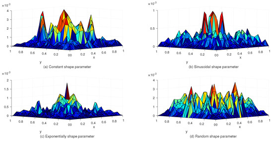
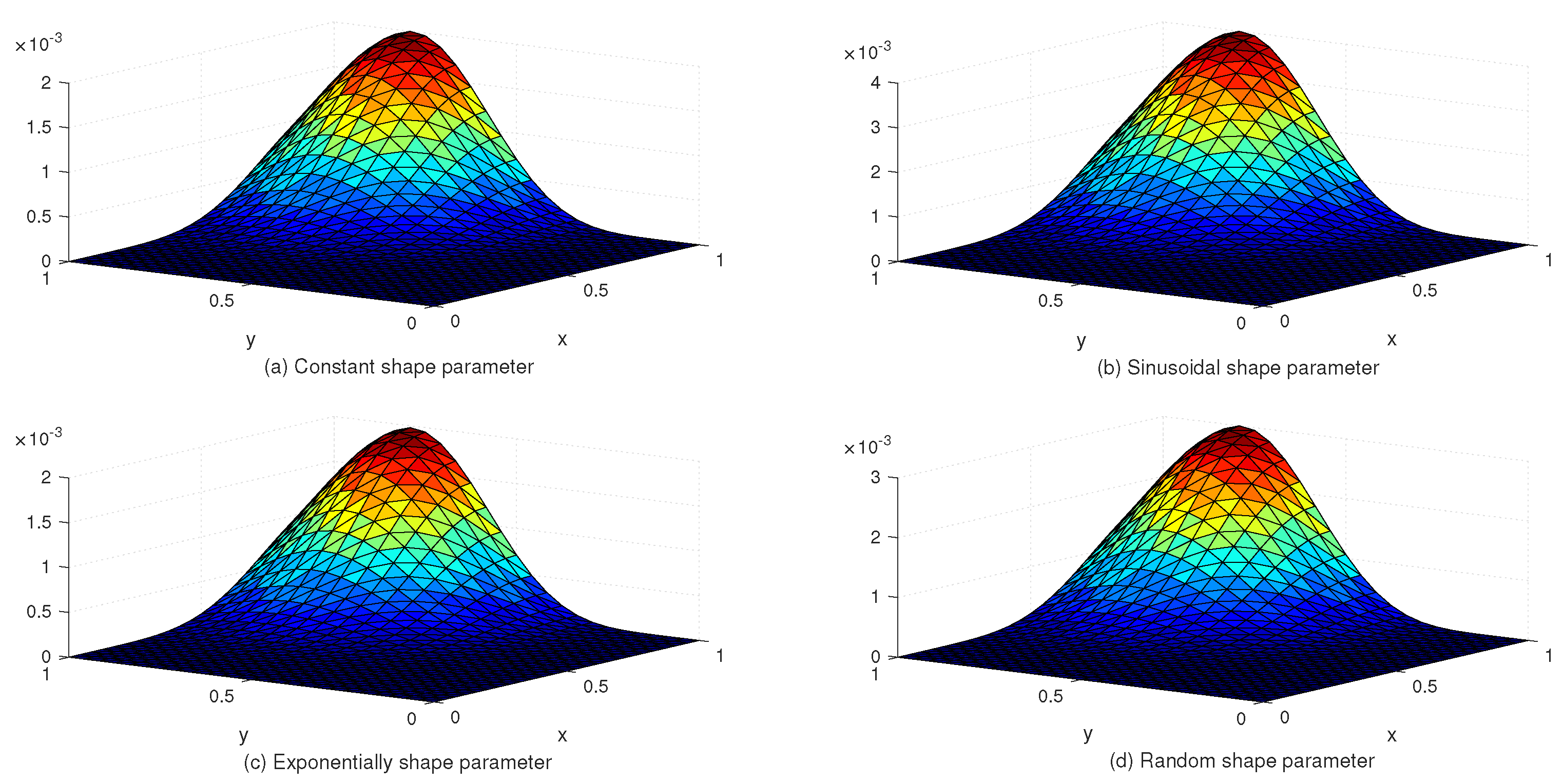
Figure 4.
The behavior of numerical errors for constant and variable SPs with in Example 1.
Example 2.
Consider the following 2DVP
with the BCs
so that exact solution is as:
Table 4 compares the and error norms with uniform and Chebyshev nodes at different values of c and global data centers. Figure 5 shows the exact and approximate solutions as well as the numerical errors with uniform and Chebyshev nodes at , . Finally, Figure 6 displays the behavior of the numerical errors for constant and variable SPs.
Table 4.
The and error norms for several values of c with the uniform and Chebyshev nodes in Example 2.

Figure 5.
The behavior of exact and approximate solutions as well as numerical errors with , in Example 2.

Figure 6.
The behavior of numerical errors for constant and variable SPs with in Example 2.
Example 3.
Finally, we consider the following 2DVP
with the BCs
so that the exact solution has the following form:
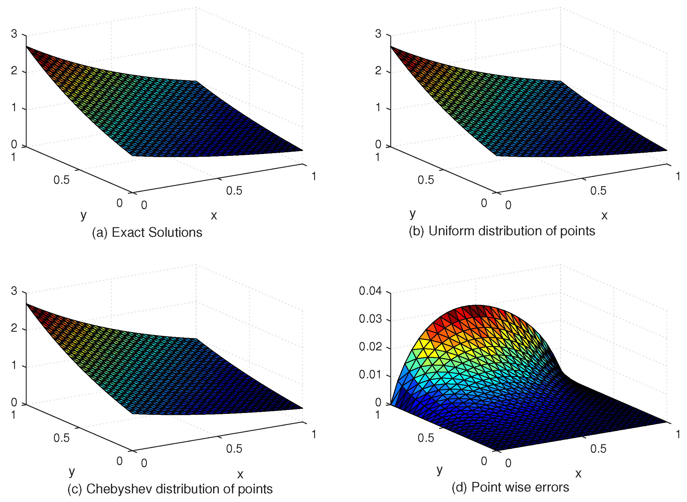
Table 5 compares the and error norms with uniform and Chebyshev nodes at different values of SPs, c and global data centers. Figure 7 shows the exact and approximate solutions as well as the numerical errors with uniform and Chebyshev nodes at , . Finally, Figure 8 displays the behavior of the numerical errors for constant and variable SPs with .
Table 5.
The and error norms for several values of c with the uniform and Chebyshev nodes in Example 3.
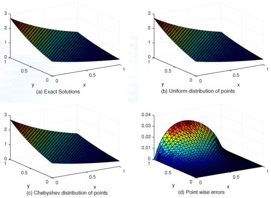
Figure 7.
The behavior of exact and approximate solutions as well as numerical errors with and in Example 3.
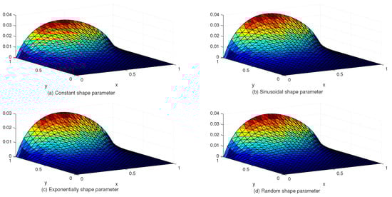
Figure 8.
The behavior of numerical errors for constant and variable SPs with in Example 3.
5. Final Remarks
Variational problems with multiple integrals occur in various applications. This paper studied the RBF collocation scheme to solve the 2DVP containing functionals that depend on the function of more than one independent variable. Moreover, this method was extended to problems of higher dimensions. The main aim of this work was to present an RBF collocation technique that did not need mesh generation to estimate the solution of 2DVP. Combining the RBF collocation technique with the Legendre–Gauss–Lobatto quadrature reduces the 2DVP to an algebraic equation system. A variable shape parameter approach was introduced for the accuracy and stability of the RBF technique. Finally, numerical experiments validated the efficiency of the presented method.
Author Contributions
Data curation, M.M.-A.; Formal analysis, A.G.; Funding acquisition, N.S.; Methodology, N.S. and M.M.-A.; Project administration, A.G.; Resources, N.S.; Writing—original draft, A.G.; Writing—review & editing, N.S. All authors have read and agreed to the published version of the manuscript.
Funding
This research received no external funding.
Data Availability Statement
Not Applicable.
Acknowledgments
The authors are thankful to the referees for their valuable comments and constructive suggestions towards the improvement of the original paper.
Conflicts of Interest
The authors declare no competing interests.
References
- Schechter, R.S. The Variational Method in Engineering; McGraw-Hill: New York, NY, USA, 1967. [Google Scholar]
- Chen, C.; Hsiao, C. A Walsh series direct method for solving variational problems. J. Frankl. Inst. 1975, 300, 265–280. [Google Scholar] [CrossRef]
- Razzaghi, M.; Yousefi, S. Legendre wavelets direct method for variational problems. Math. Comput. Simul. 2000, 53, 185–192. [Google Scholar] [CrossRef]
- Chang, R.; Wang, M. Shifted Legendre direct method for variational problems. J. Optim. Theory Appl. 1983, 39, 299–307. [Google Scholar] [CrossRef]
- Hwang, C.; Shih, Y. Laguerre series direct method for variational problems. J. Optim. Theory Appl. 1983, 39, 143–149. [Google Scholar] [CrossRef]
- Horng, I.R.; Chou, J.H. Shifted Chebyshev direct method for solving variational problems. Int. J. Syst. Sci. 1985, 16, 855–861. [Google Scholar] [CrossRef]
- Saadatmandi, A.; Abdolahi-Niasar, T. An analytic study on the Euler-Lagrange equation arising in calculus of variations. Comput. Methods Differ. Equ. 2014, 2, 140–152. [Google Scholar]
- Yousefi, S.A.; Dehghan, M. The use of He’s variational iteration method for solving variational problems. Int. J. Comput. Math. 2010, 87, 1299–1314. [Google Scholar] [CrossRef]
- Golbabai, A.; Saeedi, A. An investigation of radial basis function approximation methods with application in dynamic investment model. Iran. J. Sci. Technol. 2015, 39, 221. [Google Scholar]
- Hardy, R.L. Multiquadric equations of topography and other irregular surfaces. J. Geophys. Res. 1971, 76, 1905–1915. [Google Scholar] [CrossRef]
- Kansa, E.J. Multiquadrics—A scattered data approximation scheme with applications to computational fluid-dynamics—I surface approximations and partial derivative estimates. Comput. Math. Appl. 1990, 19, 127–145. [Google Scholar] [CrossRef]
- Kansa, E.J. Multiquadrics—A scattered data approximation scheme with applications to computational fluid-dynamics—II solutions to parabolic, hyperbolic and elliptic partial differential equations. Comput. Math. Appl. 1990, 19, 147–161. [Google Scholar] [CrossRef]
- Nikan, O.; Golbabai, A.; Nikazad, T. Solitary wave solution of the nonlinear KdV-Benjamin-Bona-Mahony-Burgers model via two meshless methods. Eur. Phys. J. Plus 2019, 134, 1–14. [Google Scholar] [CrossRef]
- Golbabai, A.; Safdari-Vaighani, A. Collocation methods based on radial basis functions for the coupled Klein–Gordon–Schrödinger equations. Electron. Trans. Numer. Anal. 2012, 39, 22–31. [Google Scholar]
- Nikan, O.; Molavi-Arabshai, S.M.; Jafari, H. Numerical simulation of the nonlinear fractional regularized long-wave model arising in ion acoustic plasma waves. Discret. Contin. Dyn. Syst. S 2021, 14, 3685. [Google Scholar] [CrossRef]
- Can, N.H.; Nikan, O.; Rasoulizadeh, M.N.; Jafari, H.; Gasimov, Y.S. Numerical computation of the time non-linear fractional generalized equal width model arising in shallow water channel. Therm. Sci. 2020, 24, 49–58. [Google Scholar] [CrossRef]
- Avazzadeh, Z.; Nikan, O.; Machado, J.A.T. Solitary wave solutions of the generalized Rosenau-KdV-RLW equation. Mathematics 2020, 8, 1601. [Google Scholar] [CrossRef]
- Nikan, O.; Avazzadeh, Z.; Machado, J.T. A local stabilized approach for approximating the modified time-fractional diffusion problem arising in heat and mass transfer. J. Adv. Res. 2021, 32, 45–60. [Google Scholar] [CrossRef]
- Rasoulizadeh, M.; Ebadi, M.; Avazzadeh, Z.; Nikan, O. An efficient local meshless method for the equal width equation in fluid mechanics. Eng. Anal. Bound. Elem. 2021, 131, 258–268. [Google Scholar] [CrossRef]
- Nikan, O.; Avazzadeh, Z.; Machado, J.T. An efficient local meshless approach for solving nonlinear time-fractional fourth-order diffusion model. J. King Saud Univ. Sci. 2021, 33, 101243. [Google Scholar] [CrossRef]
- Nikan, O.; Avazzadeh, Z.; Machado, J.T. Numerical study of the nonlinear anomalous reaction-subdiffusion process arising in the electroanalytical chemistry. J. Comput. Sci. 2021, 53, 101394. [Google Scholar] [CrossRef]
- Nikan, O.; Avazzadeh, Z. An improved localized radial basis-pseudospectral method for solving fractional reaction–subdiffusion problem. Results Phys. 2021, 23, 104048. [Google Scholar] [CrossRef]
- Rasoulizadeh, M.; Nikan, O.; Avazzadeh, Z. The impact of LRBF-FD on the solutions of the nonlinear regularized long wave equation. Math. Sci. 2021, 15, 365–376. [Google Scholar] [CrossRef]
- Nikan, O.; Avazzadeh, Z.; Machado, J.T. Numerical approximation of the nonlinear time-fractional telegraph equation arising in neutron transport. Commun. Nonlinear Sci. Numer. Simul. 2021, 99, 105755. [Google Scholar] [CrossRef]
- Nikan, O.; Avazzadeh, Z.; Machado, J.T. Numerical simulation of a degenerate parabolic problem occurring in the spatial diffusion of biological population. Chaos Solit. Fractals 2021, 151, 111220. [Google Scholar] [CrossRef]
- Nikan, O.; Avazzadeh, Z. An efficient localized meshless technique for approximating nonlinear sinh-Gordon equation arising in surface theory. Eng. Anal. Bound. Elem. 2021, 130, 268–285. [Google Scholar] [CrossRef]
- Nikan, O.; Avazzadeh, Z.; Rasoulizadeh, M. Soliton solutions of the nonlinear sine-Gordon model with Neumann boundary conditions arising in crystal dislocation theory. Nonlinear Dyn. 2021, 106, 783–813. [Google Scholar] [CrossRef]
- Nikan, O.; Avazzadeh, Z. A localisation technique based on radial basis function partition of unity for solving Sobolev equation arising in fluid dynamics. Appl. Math. Comput. 2021, 401, 126063. [Google Scholar] [CrossRef]
- Nikan, O.; Avazzadeh, Z.; Rasoulizadeh, M. Soliton wave solutions of nonlinear mathematical models in elastic rods and bistable surfaces. Eng. Anal. Bound. Elem. 2022, 143, 14–27. [Google Scholar] [CrossRef]
- Nikan, O.; Avazzadeh, Z.; Machado, J.T. Numerical treatment of microscale heat transfer processes arising in thin films of metals. Int. Commun. Heat Mass Transf. 2022, 132, 105892. [Google Scholar] [CrossRef]
- Nikan, O.; Avazzadeh, Z. Coupling of the Crank–Nicolson scheme and localized meshless technique for viscoelastic wave model in fluid flow. J. Comput. Appl. Math. 2021, 398, 113695. [Google Scholar] [CrossRef]
- Nikan, O.; Avazzadeh, Z. A locally stabilized radial basis function partition of unity technique for the sine–Gordon system in nonlinear optics. Math. Comput. Simul. 2022, 199, 394–413. [Google Scholar] [CrossRef]
- Nikan, O.; Avazzadeh, Z.; Machado, J.; Rasoulizadeh, M. An accurate localized meshfree collocation technique for the telegraph equation in propagation of electrical signals. Eng. Comput. 2022, 1–18. [Google Scholar] [CrossRef]
- Nikan, O.; Avazzadeh, Z.; Machado, J.T. Numerical approach for modeling fractional heat conduction in porous medium with the generalized Cattaneo model. Appl. Math. Model. 2021, 100, 107–124. [Google Scholar] [CrossRef]
- Nikan, O.; Avazzadeh, Z. Numerical simulation of fractional evolution model arising in viscoelastic mechanics. Appl. Numer. Math. 2021, 169, 303–320. [Google Scholar] [CrossRef]
- Buhmann, M.D. Radial Basis Functions: Theory and Implementations; Cambridge University Press: Cambridge, UK, 2003; Volume 12. [Google Scholar]
- Wendland, H. Scattered Data Approximation; Cambridge University Press: Cambridge, UK, 2005. [Google Scholar]
- Micchelli, C.A. Interpolation of scattered data: Distance matrices and conditionally positive definite functions. In Approximation Theory and Spline Functions; Springer: Berlin/Heidelberg, Germany, 1984; pp. 143–145. [Google Scholar]
- Franke, R. A Critical Comparison of Some Methods for Interpolation of Scattered Data; Technical Report; Naval Postgraduate School: Monterey, CA, USA, 1979. [Google Scholar]
- Golbabai, A.; Rabiei, H. A meshfree method based on radial basis functions for the eigenvalues of transient Stokes equations. Eng. Anal. Bound. Elem. 2012, 36, 1555–1559. [Google Scholar] [CrossRef]
- Sarra, S.A.; Sturgill, D. A random variable shape parameter strategy for radial basis function approximation methods. Eng. Anal. Bound. Elem. 2009, 33, 1239–1245. [Google Scholar] [CrossRef]
- Mirinejad, H.; Inanc, T. An RBF collocation method for solving optimal control problems. Robot. Auton. Syst. 2017, 87, 219–225. [Google Scholar] [CrossRef]
- Rad, J.A.; Kazem, S.; Parand, K. Radial basis functions approach on optimal control problems: A numerical investigation. J. Vib. Control 2014, 20, 1394–1416. [Google Scholar] [CrossRef]
- Canuto, C.; Hussaini, M.Y.; Quarteroni, A.; Zang, T.A. Spectral Methods: Fundamentals in Single Domains; Springer Science & Business Media: Berlin/Heidelberg, Germany, 2007. [Google Scholar]


Publisher’s Note: MDPI stays neutral with regard to jurisdictional claims in published maps and institutional affiliations. |
© 2022 by the authors. Licensee MDPI, Basel, Switzerland. This article is an open access article distributed under the terms and conditions of the Creative Commons Attribution (CC BY) license (https://creativecommons.org/licenses/by/4.0/).