

Characterizing Microheterogeneity in Liquid Mixtures via Local Density Fluctuations


Abstract
1. Introduction
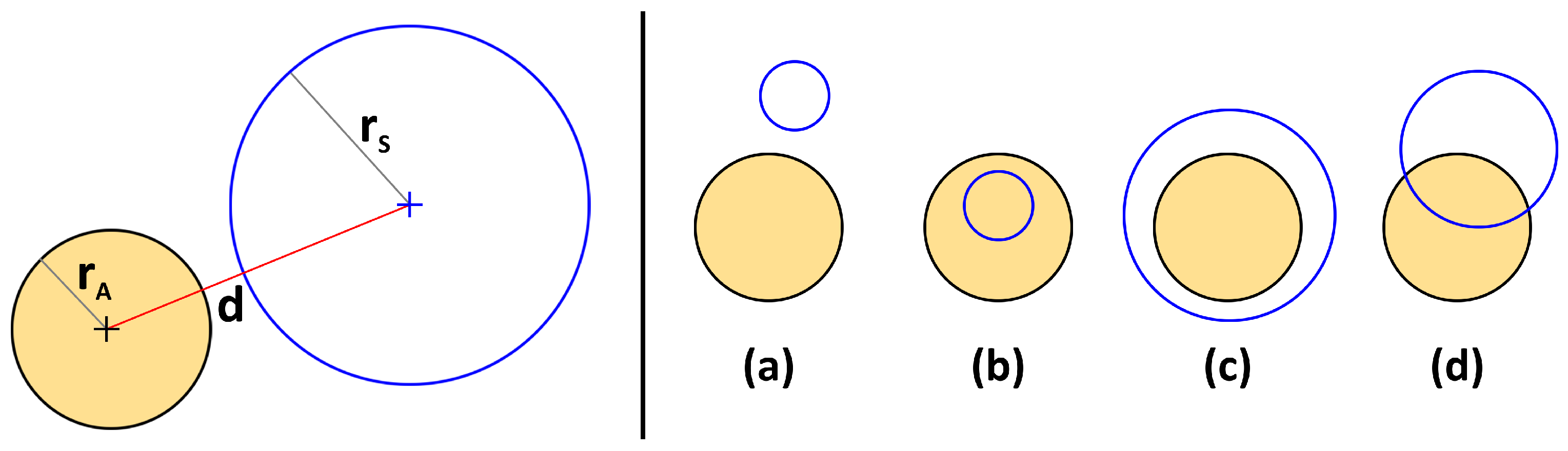
2. Proposed Method
- (a)
- If : Disjunct
- (b)
- If and : Sphere contained in atom
- (c)
- If and : Atom contained in sphere
- (d)
- Else: Partial overlap
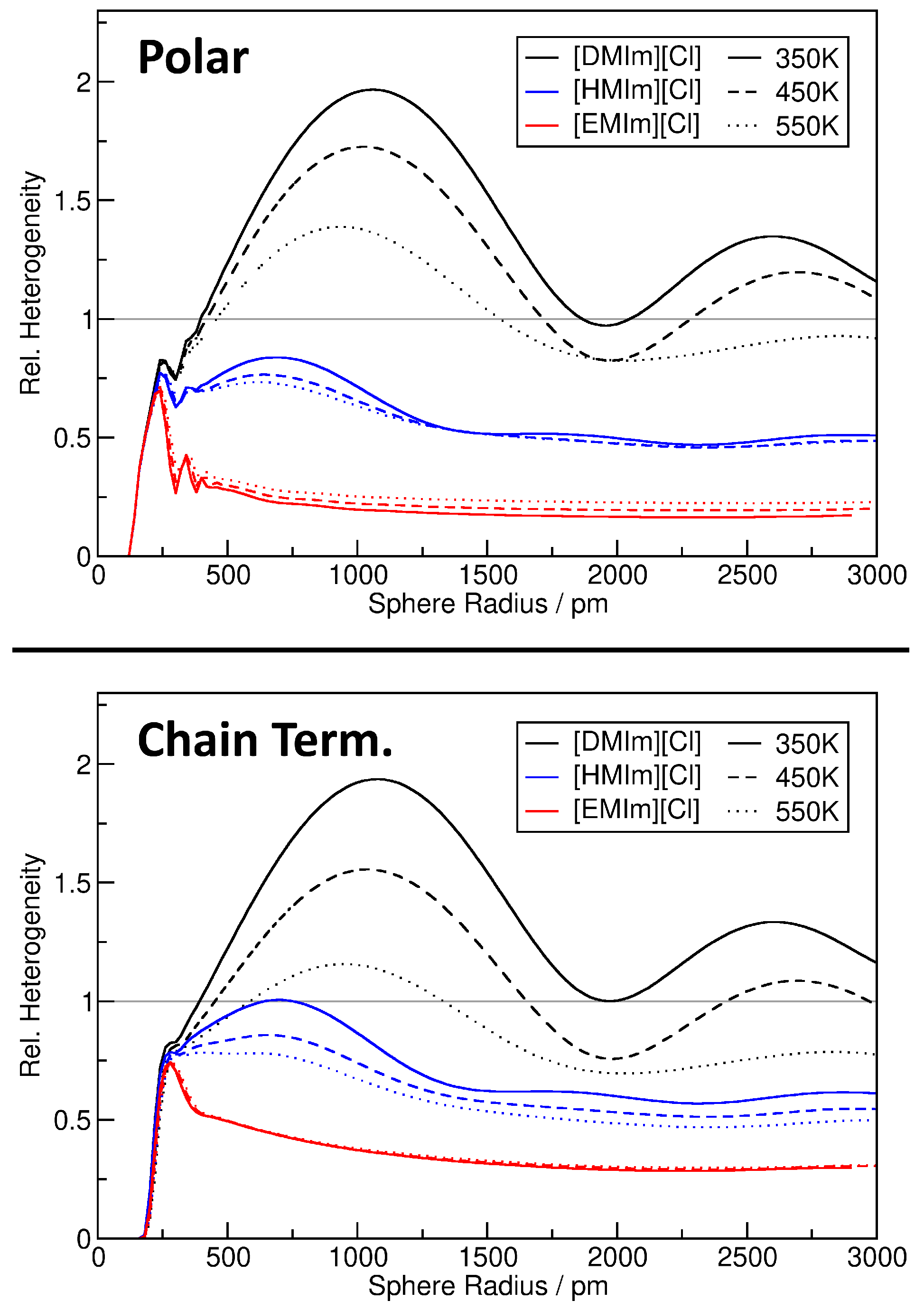
2.1. Quantifying Heterogeneity
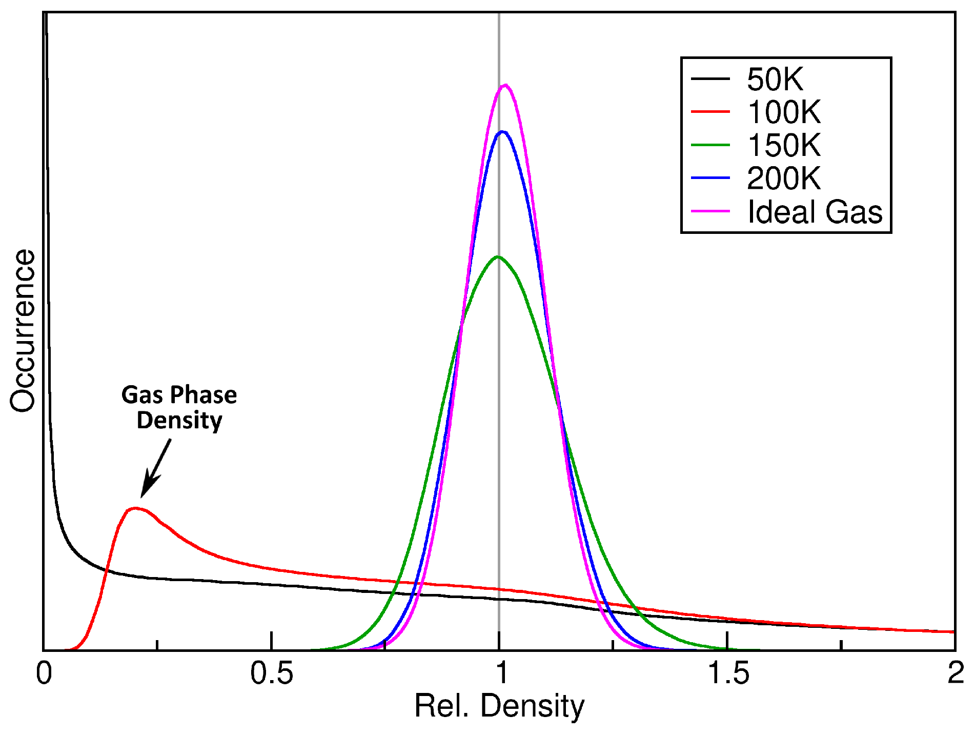
2.2. Ideal Gas as a Reference
2.3. Estimating Configuration Entropy
2.4. Multiple Observations
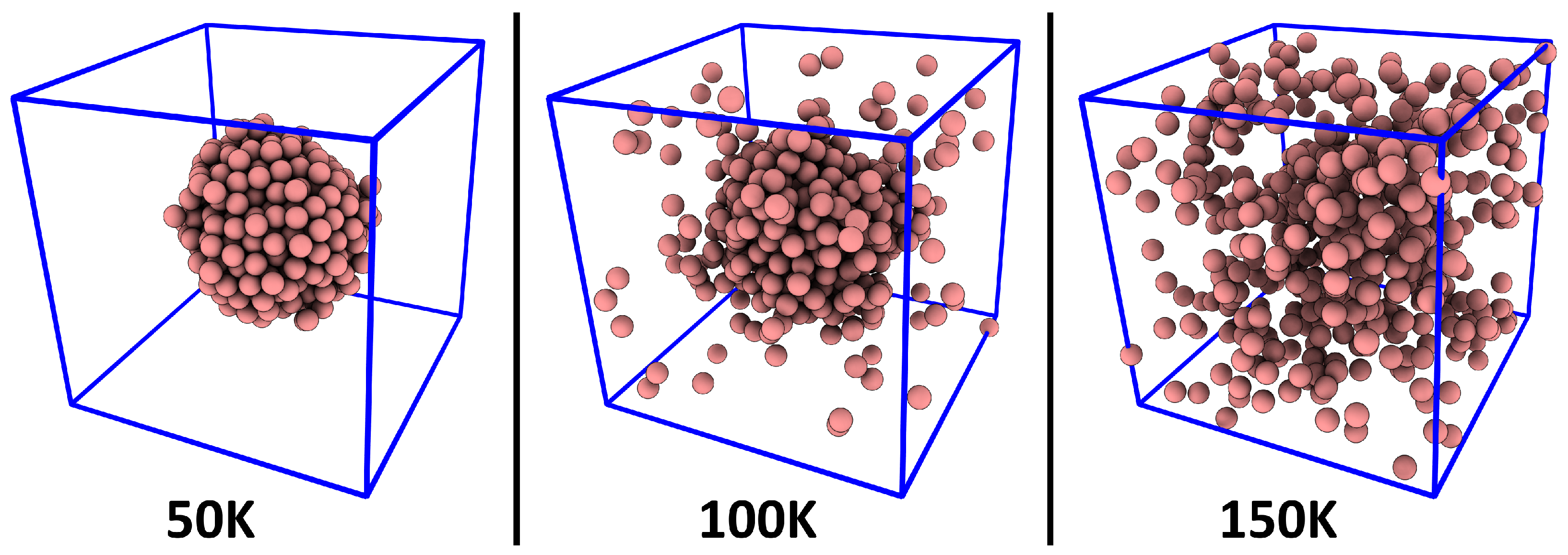
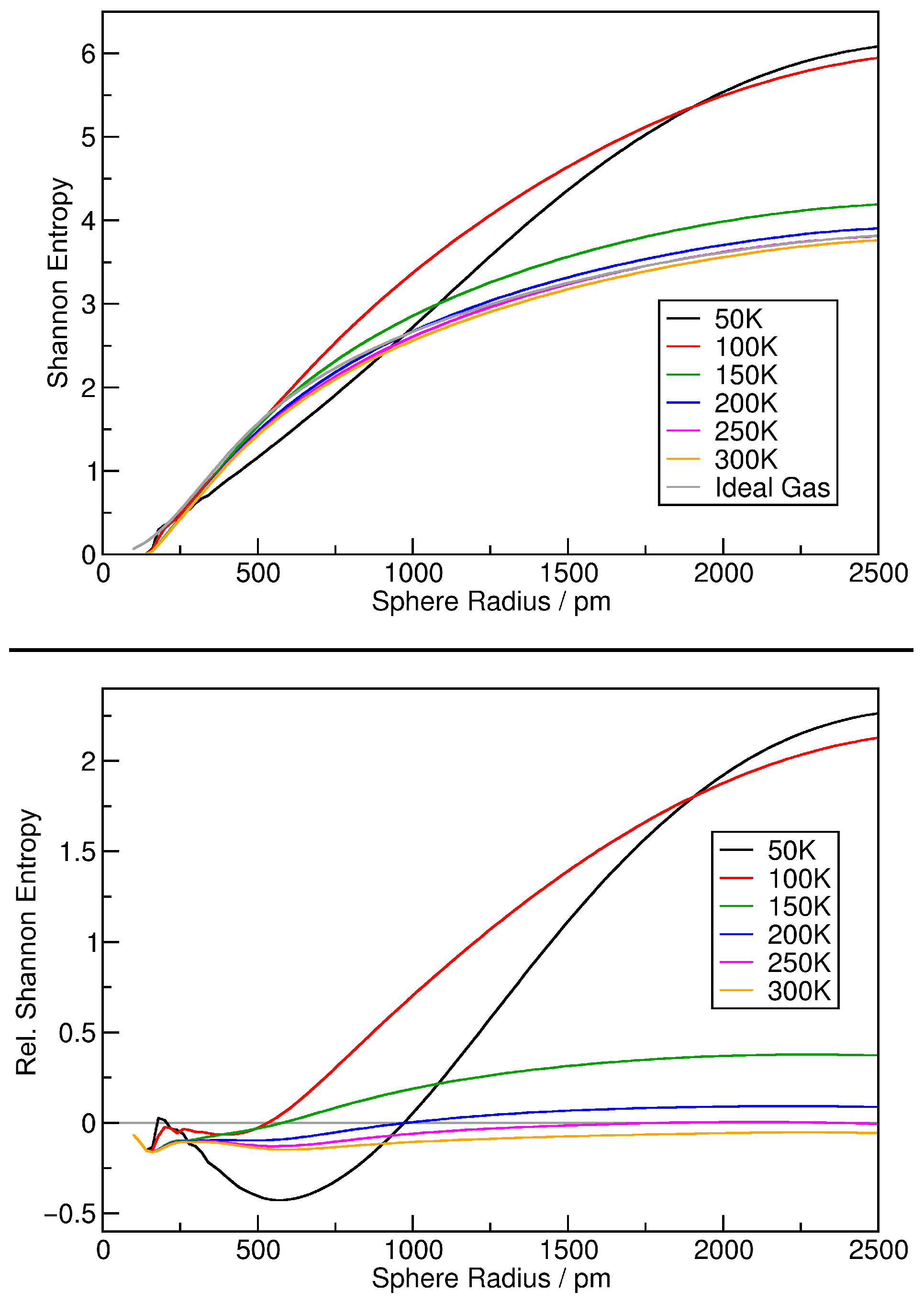
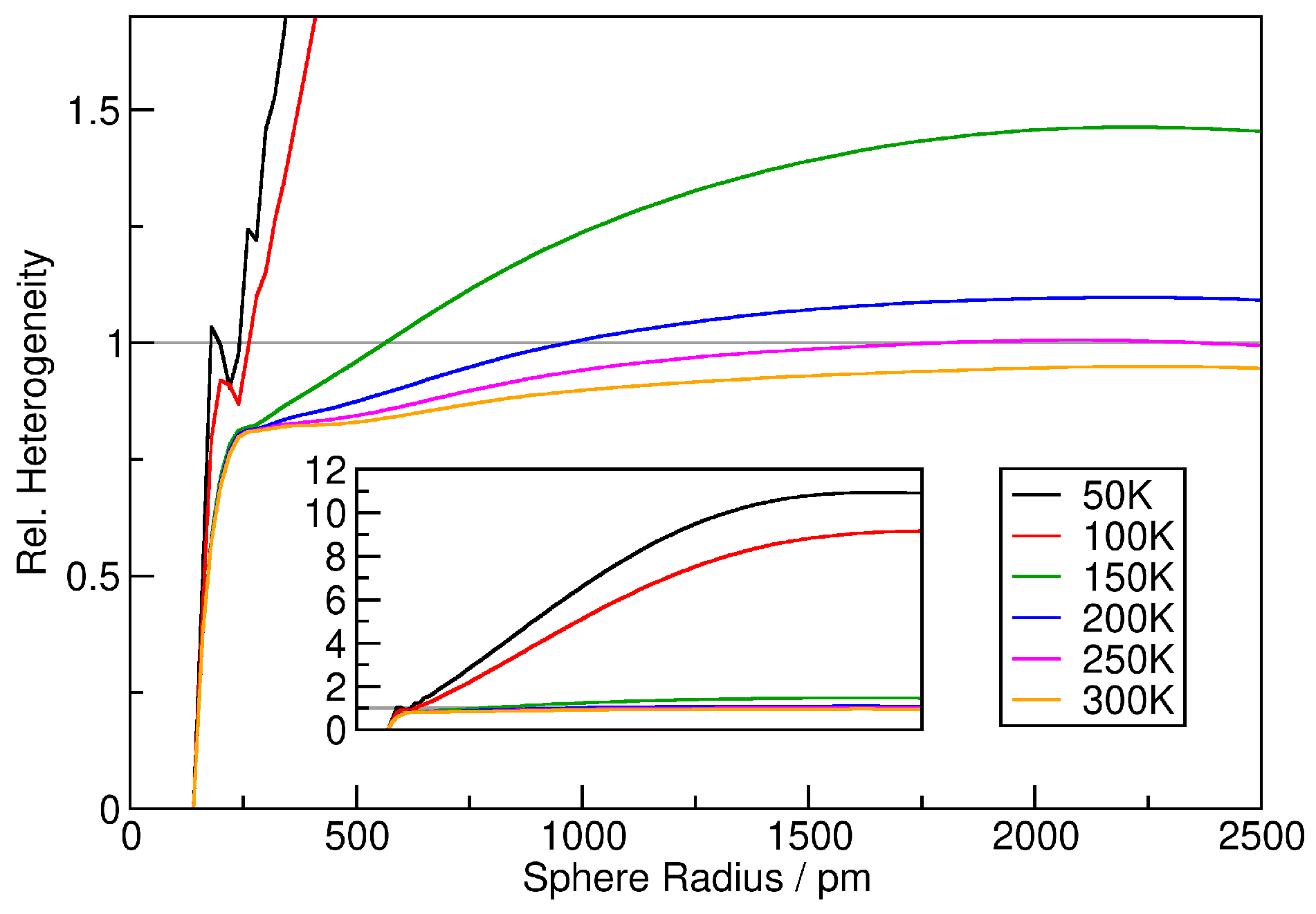
3. Verification: Argon
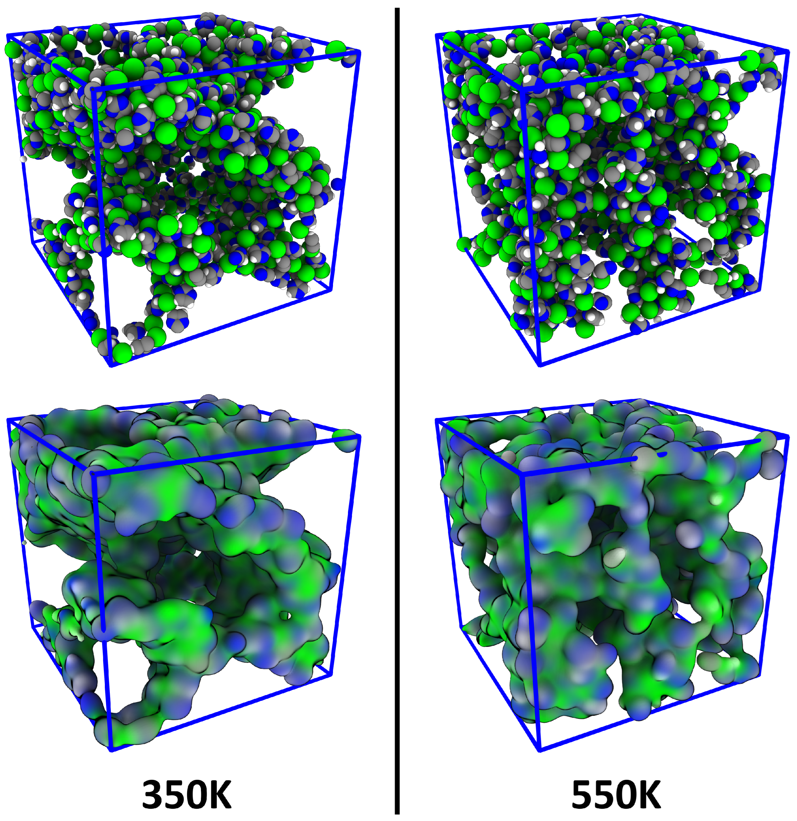
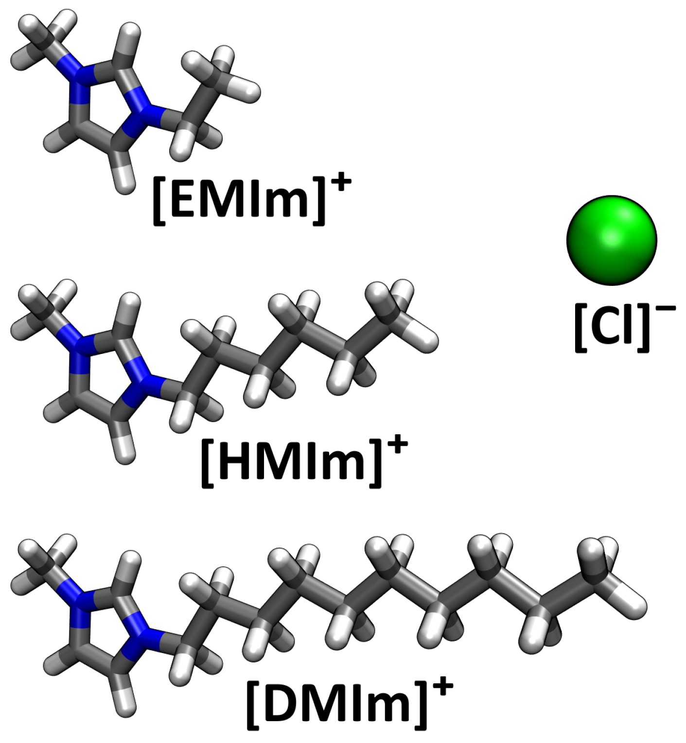
4. Application: Ionic Liquids
4.1. Investigating Voids
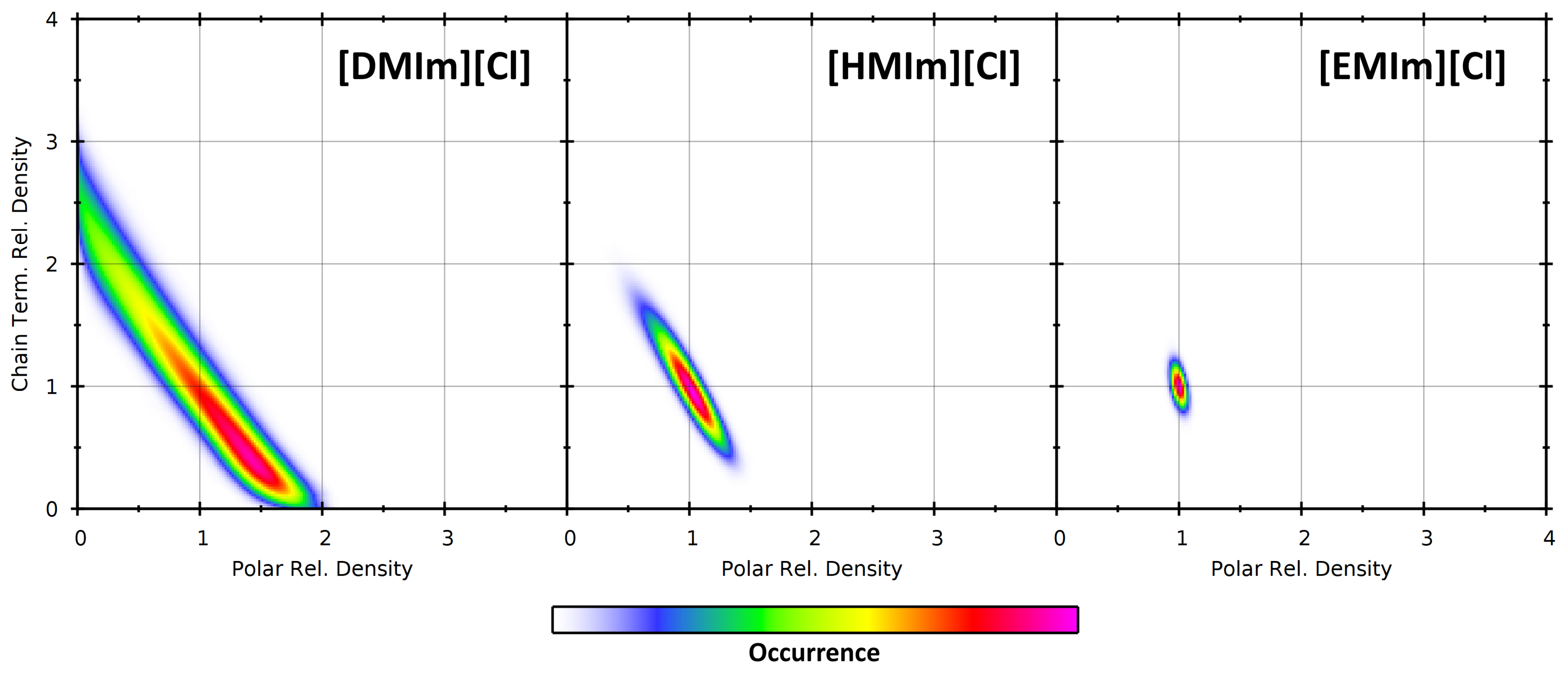
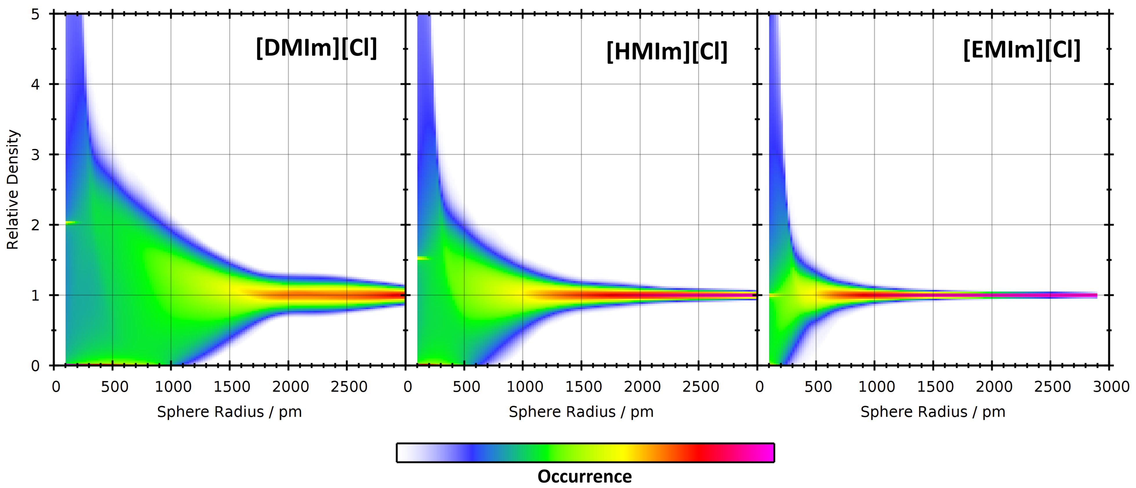
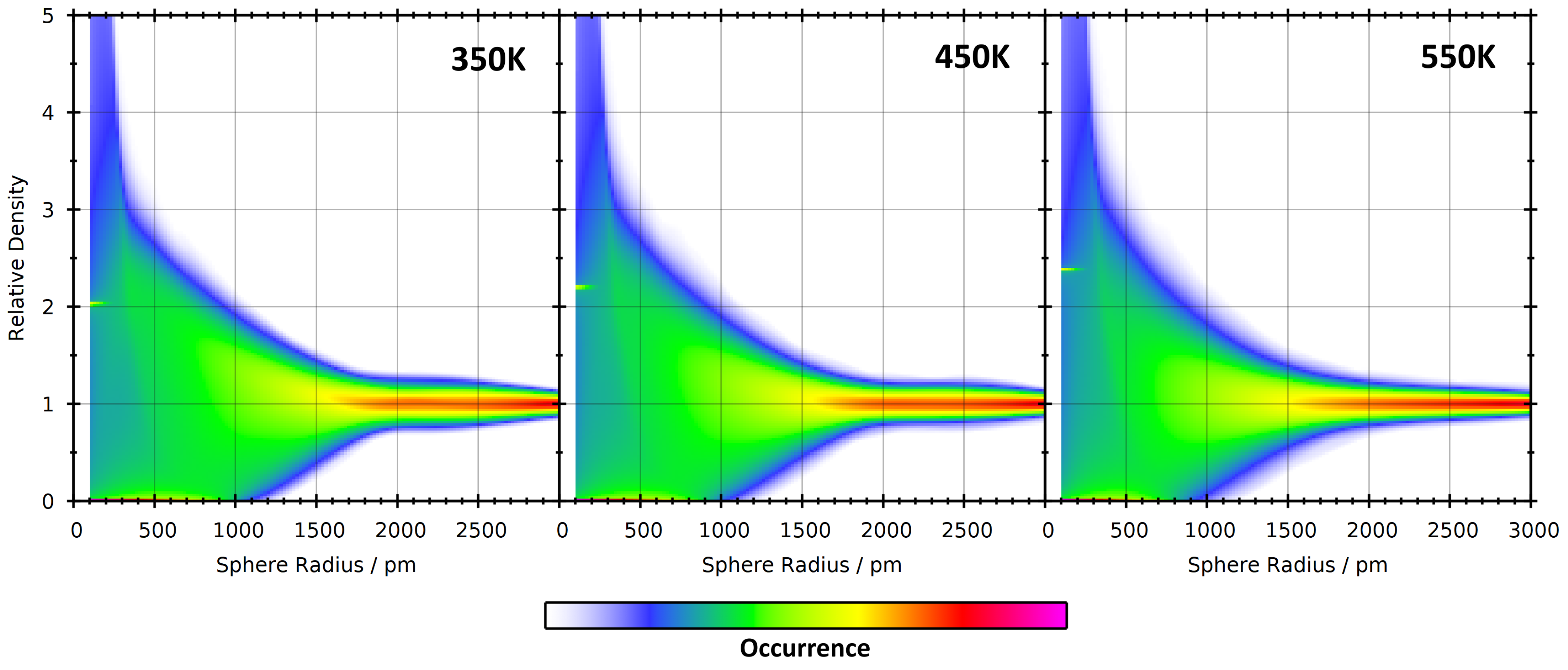
4.2. Partial Density Correlation
4.3. Comparison to Voronoi-Based Domain Analysis
5. Computational Details
- 25 ps NVT simulation at 500 K, using a Berendsen thermostat [64] with a coupling constant of 1.0 fs.
- 500 ps NVT simulation at target temperature.
- 500 ps NVT simulation, using a Nosé–Hoover thermostat with a coupling constant of 100 fs.
- 1 ns NpT simulation, using a Nosé–Hoover thermostat with a coupling constant of 100 fs and a Nosé–Hoover barostat with a coupling constant of 2000 fs.
- 1 ns NpT simulation, using a Langevin thermostat with a coupling constant of 100 fs (to dampen possible shock waves) and a Nosé–Hoover barostat with a coupling constant of 2000 fs.
- 15 ns NpT simulation, using a Nosé–Hoover thermostat with a coupling constant of 100 fs and a Nosé–Hoover barostat with a coupling constant of 2000 fs.
- 15 ns NpT simulation, using a Nosé–Hoover thermostat with a coupling constant of 100 fs and a Nosé–Hoover barostat with a coupling constant of 2000 fs. The average density is computed during this run.
- 1 ns simulation to monotonously shrink/grow the simulation cell to match the target density from the averaging, using a Nosé–Hoover thermostat with a coupling constant of 100 fs.
- 1 ns NVT simulation, using a Langevin thermostat with a coupling constant of 100 fs to dampen possible shock waves.
- 80 ns NVT simulation (final equilibration), using a Nosé–Hoover thermostat with a coupling constant of 100 fs.
- 30 ns NVT simulation (production run).
6. Conclusions
Author Contributions
Funding
Institutional Review Board Statement
Informed Consent Statement
Data Availability Statement
Acknowledgments
Conflicts of Interest
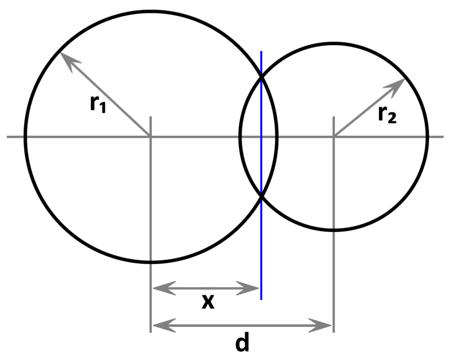
Appendix A. Derivation of Sphere Intersection Volume
References
- Walden, P. Molecular weights and electrical conductivity of several fused salts. Bull. Acad. Imp. Sci. 1914, 1800, 405–422. [Google Scholar]
- Malberg, F.; Brehm, M.; Hollóczki, O.; Pensado, A.S.; Kirchner, B. Understanding the evaporation of ionic liquids using the example of 1-ethyl-3-methylimidazolium ethylsulfate. Phys. Chem. Chem. Phys. 2013, 15, 18424. [Google Scholar] [CrossRef] [PubMed]
- Sarmiento, G.P.; Zelcer, A.; Espinosa, M.S.; Babay, P.A.; Mirenda, M. Photochemistry of imidazolium cations. Water addition to methylimidazolium ring induced by UV radiation in aqueous solution. J. Photochem. Photobiol. A 2016, 314, 155–163. [Google Scholar] [CrossRef]
- Alpers, T.; Muesmann, T.W.T.; Temme, O.; Christoffers, J. Perfluorinated 1,2,3- and 1,2,4-Triazolium Ionic Liquids. Eur. J. Org. Chem. 2018, 2018, 4331–4337. [Google Scholar] [CrossRef]
- Akbey, Ü.; Granados-Focil, S.; Coughlin, E.B.; Graf, R.; Spiess, H.W. 1H Solid-State NMR Investigation of Structure and Dynamics of Anhydrous Proton Conducting Triazole-Functionalized Siloxane Polymers. J. Phys. Chem. B 2009, 113, 9151–9160. [Google Scholar] [CrossRef] [PubMed]
- Roohi, H.; Salehi, R. Molecular engineering of the electronic, structural, and electrochemical properties of nanostructured 1-methyl-4-phenyl-1, 2, 4-triazolium-based [PhMTZ][X 1–10] ionic liquids through anionic changing. Ionics 2018, 24, 483–504. [Google Scholar] [CrossRef]
- Egorova, K.S.; Seitkalieva, M.M.; Posvyatenko, A.V.; Khrustalev, V.N.; Ananikov, V.P. Cytotoxic Activity of Salicylic Acid-Containing Drug Models with Ionic and Covalent Binding. ACS Med. Chem. Lett. 2015, 6, 1099–1104. [Google Scholar] [CrossRef] [PubMed]
- Pinto, P.C.A.G.; Ribeiro, D.M.G.P.; Azevedo, A.M.O.; Dela Justina, V.; Cunha, E.; Bica, K.; Vasiloiu, M.; Reis, S.; Saraiva, M.L.M.F.S. Active pharmaceutical ingredients based on salicylate ionic liquids: Insights into the evaluation of pharmaceutical profiles. New J. Chem. 2013, 37, 4095–4102. [Google Scholar] [CrossRef]
- Stappert, K.; Ünal, D.; Spielberg, E.T.; Mudring, A.V. Influence of the Counteranion on the Ability of 1-Dodecyl-3-methyltriazolium Ionic Liquids to Form Mesophases. Cryst. Growth Des. 2015, 15, 752–758. [Google Scholar] [CrossRef]
- Payal, R.S.; Bejagam, K.K.; Mondal, A.; Balasubramanian, S. Dissolution of Cellulose in Room Temperature Ionic Liquids: Anion Dependence. J. Phys. Chem. B 2015, 119, 1654–1659. [Google Scholar] [CrossRef]
- Gardas, R.L.; Costa, H.F.; Freire, M.G.; Carvalho, P.J.; Marrucho, I.M.; Fonseca, I.M.A.; Ferreira, A.G.M.; Coutinho, J.A.P. Densities and Derived Thermodynamic Properties of Imidazolium-, Pyridinium-, Pyrrolidinium-, and Piperidinium-based Ionic Liquids. J. Chem. Eng. Data 2008, 53, 805–811. [Google Scholar] [CrossRef]
- Sanchez, L.G.; Espel, J.R.; Onink, F.; Meindersma, G.W.; de Haan, A.B. Density, Viscosity, and Surface Tension of Synthesis Grade Imidazolium, Pyridinium, and Pyrrolidinium Based Room Temperature Ionic Liquids. J. Chem. Eng. Data 2009, 54, 2803–2812. [Google Scholar] [CrossRef]
- Castner, E.W., Jr.; Wishart, J.F. Spotlight on Ionic Liquids. J. Chem. Phys. 2010, 132, 120901. [Google Scholar] [CrossRef] [PubMed]
- Siedlecka, E.M.; Czerwicka, M.; Stolte, S.; Stepnowski, P. Stability of Ionic Liquids in Application Conditions. Curr. Org. Chem. 2011, 15, 1974–1991. [Google Scholar] [CrossRef]
- Kiefer, J.; Obert, K.; Boesmann, A.; Seeger, T.; Wasserscheid, P.; Leipertz, A. Quantitative Analysis of Alpha-d-glucose in an Ionic Liquid by Using Infrared Spectroscopy. ChemPhysChem 2008, 9, 1317–1322. [Google Scholar] [CrossRef] [PubMed]
- Fumino, K.; Wulf, A.; Ludwig, R. The Potential Role of Hydrogen Bonding in Aprotic and Protic Ionic Liquids. Phys. Chem. Chem. Phys. 2009, 11, 8790–8794. [Google Scholar] [CrossRef] [PubMed]
- Kempter, V.; Kirchner, B. The Role of Hydrogen Atoms in Interactions Involving Imidazolium-based Ionic Liquids. J. Mol. Struct. 2010, 972, 22–34. [Google Scholar] [CrossRef]
- Peppel, T.; Roth, C.; Fumino, K.; Paschek, D.; Koeckerling, M.; Ludwig, R. The Influence of Hydrogen-bond Defects on the Properties of Ionic Liquids. Angew. Chem. Int. Ed. 2011, 50, 6661–6665. [Google Scholar] [CrossRef] [PubMed]
- Youngs, T.G.A.; Holbrey, J.D.; Mullan, C.L.; Norman, S.E.; Lagunas, M.C.; D’Agostino, C.; Mantle, M.D.; Gladden, L.F.; Bowron, D.T.; Hardacre, C. Neutron Diffraction, NMR and Molecular Dynamics Study of Glucose Dissolved in the Ionic Liquid 1-ethyl-3-methylimidazolium Acetate. Chem. Sci. 2011, 2, 1594–1605. [Google Scholar] [CrossRef]
- Zhang, Y.; Chan, J.Y.G. Sustainable Chemistry: Imidazolium Salts in Biomass Conversion and CO2 Fixation. Energy Environ. Sci. 2010, 3, 408–417. [Google Scholar] [CrossRef]
- Sescousse, R.; Le, K.A.; Ries, M.E.; Budtova, T. Viscosity of Cellulose-imidazolium-based Ionic Liquid Solutions. J. Phys. Chem. B 2010, 114, 7222–7228. [Google Scholar] [CrossRef] [PubMed]
- Brandt, A.; Hallett, J.P.; Leak, D.J.; Murphy, R.J.; Welton, T. The Effect of the Ionic Liquid Anion in the Pretreatment of Pine Wood Chips. Green Chem. 2010, 12, 672–679. [Google Scholar] [CrossRef]
- Du, H.; Qian, X. The Effects of Acetate Anion on Cellulose Dissolution and Reaction in Imidazolium Ionic Liquids. Carbohydr. Res. 2011, 346, 1985–1990. [Google Scholar] [CrossRef] [PubMed]
- Qin, Y.; Lu, X.; Sun, N.; Rogers, R.D. Dissolution or Extraction of Crustacean Shells Using Ionic Liquids to Obtain High Molecular Weight Purified Chitin and Direct Production of Chitin Films and Fibers. Green Chem. 2011, 12, 968–971. [Google Scholar] [CrossRef]
- Shiflett, M.B.; Yokozeki, A. Phase Behavior of Carbon Dioxide in Ionic Liquids: [emim][acetate], [emim][trifluoroacetate], and [emim][acetate] Plus [emim][trifluoroacetate] Mixtures. J. Chem. Eng. Data 2009, 54, 108–114. [Google Scholar] [CrossRef]
- Canongia Lopes, J.N.A.; Pádua, A.A.H. Nanostructural Organization in Ionic Liquids. J. Phys. Chem. B 2006, 110, 3330–3335. [Google Scholar] [CrossRef]
- Patra, S.; Samanta, A. Microheterogeneity of Some Imidazolium Ionic Liquids As Revealed by Fluorescence Correlation Spectroscopy and Lifetime Studies. J. Phys. Chem. B 2012, 116, 12275–12283. [Google Scholar] [CrossRef] [PubMed]
- Brehm, M.; Weber, H.; Pensado, A.S.; Stark, A.; Kirchner, B. Liquid Structure and Cluster Formation in Ionic Liquid/Water Mixtures – An Extensive ab initio Molecular Dynamics Study on 1-Ethyl-3-Methylimidazolium Acetate/Water Mixtures—Part. Z. Phys. Chem. 2013, 227, 177–204. [Google Scholar] [CrossRef]
- Hollóczki, O.; Macchiagodena, M.; Weber, H.; Thomas, M.; Brehm, M.; Stark, A.; Russina, O.; Triolo, A.; Kirchner, B. Triphilic Ionic-Liquid Mixtures: Fluorinated and Non-Fluorinated Aprotic Ionic-Liquid Mixtures. ChemPhysChem 2015, 16, 3325–3333. [Google Scholar] [CrossRef]
- Elfgen, R.; Hollóczki, O.; Kirchner, B. A Molecular Level Understanding of Template Effects in Ionic Liquids. Acc. Chem. Res. 2017, 50, 2949–2957. [Google Scholar] [CrossRef]
- Panja, S.K.; Saha, S. Microheterogeneity in imidazolium and piperidinium cation-based ionic liquids: 1D and 2D NMR studies. Magn. Reson. Chem. 2017, 56, 95–102. [Google Scholar] [CrossRef] [PubMed]
- Brehm, M.; Sebastiani, D. Simulating structure and dynamics in small droplets of 1-ethyl-3-methylimidazolium acetate. J. Chem. Phys. 2018, 148, 193802. [Google Scholar] [CrossRef] [PubMed]
- Alizadeh, V.; Geller, D.; Malberg, F.; Sánchez, P.B.; Padua, A.; Kirchner, B. Strong Microheterogeneity in Novel Deep Eutectic Solvents. ChemPhysChem 2019, 20, 1786–1792. [Google Scholar] [CrossRef]
- Ray, P.; Elfgen, R.; Kirchner, B. Cation influence on heterocyclic ammonium ionic liquids: A molecular dynamics study. Phys. Chem. Chem. Phys. 2019, 21, 4472–4486. [Google Scholar] [CrossRef] [PubMed]
- Zhao, R.; Xu, X.; Wang, Z.; Zheng, Y.; Zhou, Y.; Yu, Z. Structural microheterogeneity and hydrogen bonding properties in the mixtures of two ionic liquids with a common imidazolium cation. J. Mol. Liq. 2022, 368, 120594. [Google Scholar] [CrossRef]
- Biswas, A.; Mallik, B.S. Microheterogeneity-Induced Vibrational Spectral Dynamics of Aqueous 1-Alkyl-3-methylimidazolium Tetrafluoroborate Ionic Liquids of Different Cationic Chain Lengths. J. Phys. Chem. B 2022, 126, 5523–5533. [Google Scholar] [CrossRef] [PubMed]
- Almásy, L.; Kuklin, A.I.; Požar, M.; Baptista, A.; Perera, A. Microscopic origin of the scattering pre-peak in aqueous propylamine mixtures: X-ray and neutron experiments versus simulations. Phys. Chem. Chem. Phys. 2019, 21, 9317–9325. [Google Scholar] [CrossRef] [PubMed]
- Ciach, A. Mesoscopic theory for inhomogeneous mixtures. Mol. Phys. 2011, 109, 1101–1119. [Google Scholar] [CrossRef]
- Santos, A.P.; Pȩkalski, J.; Panagiotopoulos, A.Z. Thermodynamic signatures and cluster properties of self-assembly in systems with competing interactions. Soft Matter 2017, 13, 8055–8063. [Google Scholar] [CrossRef]
- Frömbgen, T.; Blasius, J.; Alizadeh, V.; Chaumont, A.; Brehm, M.; Kirchner, B. Cluster Analysis in Liquids: A Novel Tool in TRAVIS. J. Chem. Inf. Model. 2022, 62, 5634–5644. [Google Scholar] [CrossRef]
- Brehm, M.; Weber, H.; Thomas, M.; Hollóczki, O.; Kirchner, B. Domain Analysis in Nanostructured Liquids: A Post-Molecular Dynamics Study at the Example of Ionic Liquids. ChemPhysChem 2015, 16, 3271–3277. [Google Scholar] [CrossRef] [PubMed]
- Mendez-Morales, T.; Li, Z.; Salanne, M. Computational Screening of the Physical Properties of Water-in-Salt Electrolytes. Batter. Supercaps 2020, 4, 646–652. [Google Scholar] [CrossRef]
- Gehrke, S.; Ray, P.; Stettner, T.; Balducci, A.; Kirchner, B. Water in Protic Ionic Liquid Electrolytes: From Solvent Separated Ion Pairs to Water Clusters. ChemSusChem 2021, 14, 3315–3324. [Google Scholar] [CrossRef] [PubMed]
- Mazzilli, V.; Wang, Y.; Saielli, G. The structuring effect of the alkyl domains on the polar network of ionic liquid mixtures: A molecular dynamics study. Phys. Chem. Chem. Phys. 2022, 24, 18783–18792. [Google Scholar] [CrossRef] [PubMed]
- Dick, L.; Stettner, T.; Liu, Y.; Liu, S.; Kirchner, B.; Balducci, A. Hygroscopic protic ionic liquids as electrolytes for electric double layer capacitors. Energy Storage Mater. 2022, 53, 744–753. [Google Scholar] [CrossRef]
- Brehm, M.; Kirchner, B. TRAVIS—A free analyzer and visualizer for Monte Carlo and molecular dynamics trajectories. J. Chem. Inf. Model. 2011, 51, 2007–2023. [Google Scholar] [CrossRef] [PubMed]
- Brehm, M.; Thomas, M.; Gehrke, S.; Kirchner, B. TRAVIS—A free analyzer for trajectories from molecular simulation. J. Chem. Phys. 2020, 152, 164105. [Google Scholar] [CrossRef] [PubMed]
- Shannon, C.E. A Mathematical Theory of Communication. Bell Syst. Tech. J. 1948, 27, 379–423. [Google Scholar] [CrossRef]
- Shannon, C.E. A Mathematical Theory of Communication. Bell Syst. Tech. J. 1948, 27, 623–656. [Google Scholar] [CrossRef]
- Pathria, R.K. Statistical Mechanics, 3rd ed.; Elsevier: Amsterdam, The Netherlands; Academic Press: Amsterdam, The Netherlands, 2011. [Google Scholar]
- Beirlant, J.; Dudewicz, E.J.; Gyorfi, L.; van der Meulen, E.C. Nonparametric entropy estimation: An overview. Int. J. Math. Sci. 1997, 6, 17–39. [Google Scholar]
- Miller, G. Note on the bias of information estimates. In Information Theory in Psychology: Problems and Methods; Free Press: New York, NY, USA, 1955; pp. 95–100. [Google Scholar]
- Bondi, A. van der Waals Volumes and Radii. J. Phys. Chem. 1964, 68, 441–451. [Google Scholar] [CrossRef]
- Rowland, R.S.; Taylor, R. Intermolecular Nonbonded Contact Distances in Organic Crystal Structures: Comparison with Distances Expected from van der Waals Radii. J. Phys. Chem. 1996, 100, 7384–7391. [Google Scholar] [CrossRef]
- Mantina, M.; Chamberlin, A.C.; Valero, R.; Cramer, C.J.; Truhlar, D.G. Consistent van der Waals Radii for the Whole Main Group. J. Phys. Chem. A 2009, 113, 5806–5812. [Google Scholar] [CrossRef]
- Plimpton, S. Fast parallel algorithms for short-range molecular dynamics. J. Comput. Phys. 1995, 117, 1–19. [Google Scholar] [CrossRef]
- Canongia Lopes, J.N.; Deschamps, J.; Pádua, A.A.H. Modeling Ionic Liquids Using a Systematic All-Atom Force Field. J. Phys. Chem. B 2004, 108, 2038–2047. [Google Scholar] [CrossRef]
- Canongia Lopes, J.N.; Pádua, A.A.H. Molecular Force Field for Ionic Liquids III: Imidazolium, Pyridinium, and Phosphonium Cations; Chloride, Bromide, and Dicyanamide Anions. J. Phys. Chem. B 2006, 110, 19586–19592. [Google Scholar] [CrossRef] [PubMed]
- Canongia Lopes, J.N.; Pádua, A.A.H. CL&P: A generic and systematic force field for ionic liquids modeling. Theor. Chem. Acc. 2012, 131, 1129. [Google Scholar] [CrossRef]
- Jorgensen, W.L.; Maxwell, D.S.; Tirado-Rives, J. Development and testing of the OPLS all-atom force field on conformational energetics and properties of organic liquids. J. Am. Chem. Soc. 1996, 118, 11225–11236. [Google Scholar] [CrossRef]
- Ponder, J.W.; Case, D.A. Force Fields for Protein Simulations. In Advances in Protein Chemistry; Elsevier: Amsterdam, The Netherlands, 2003; pp. 27–85. [Google Scholar] [CrossRef]
- Sambasivarao, S.V.; Acevedo, O. Development of OPLS-AA Force Field Parameters for 68 Unique Ionic Liquids. J. Chem. Theory Comput. 2009, 5, 1038–1050. [Google Scholar] [CrossRef]
- Martínez, L.; Andrade, R.; Birgin, E.G.; Martínez, J.M. PACKMOL: A package for building initial configurations for molecular dynamics simulations. J. Comput. Chem. 2009, 30, 2157–2164. [Google Scholar] [CrossRef]
- Berendsen, H.J.C.; Postma, J.P.M.; van Gunsteren, W.F.; DiNola, A.; Haak, J.R. Molecular dynamics with coupling to an external bath. J. Chem. Phys. 1984, 81, 3684–3690. [Google Scholar] [CrossRef]
- Nose, S. A molecular dynamics method for simulations in the canonical ensemble. Mol. Phys. 1984, 52, 255–268. [Google Scholar] [CrossRef]
- Nose, S. A unified formulation of the constant temperature molecular dynamics methods. J. Chem. Phys. 1984, 81, 511–519. [Google Scholar] [CrossRef]
- Martyna, G.; Klein, M.; Tuckerman, M. Nosé–Hoover chains: The canonical ensemble via continuous dynamics. J. Chem. Phys. 1992, 97, 2535–2643. [Google Scholar] [CrossRef]
- Schneider, T.; Stoll, E. Molecular-dynamics study of a three-dimensional one-component model for distortive phase transitions. Phys. Rev. B 1978, 17, 1302–1322. [Google Scholar] [CrossRef]
- Dünweg, B.; Paul, W. Brownian dynamics simulations without gaussian random numbers. Int. J. Mod. Phys. C 1991, 2, 817–827. [Google Scholar] [CrossRef]
- Rowley, L.; Nicholson, D.; Parsonage, N. Monte Carlo grand canonical ensemble calculation in a gas-liquid transition region for 12-6 Argon. J. Comput. Phys. 1975, 17, 401–414. [Google Scholar] [CrossRef]
- Humphrey, W.; Dalke, A.; Schulten, K. VMD: Visual molecular dynamics. J. Mol. Graph. 1996, 14, 33–38. [Google Scholar] [CrossRef]
- Stone, J. An Efficient Library for Parallel Ray Tracing and Animation. Master’s Thesis, Computer Science Department, University of Missouri-Rolla, Rolla, MO, USA, 1998. [Google Scholar]
- Williams, T.; Kelley, C. Gnuplot 6.0: An Interactive Plotting Program. 2023. Available online: http://gnuplot.sourceforge.net/ (accessed on 23 January 2024).
- Grace Development Team. 1996. Available online: http://plasma-gate.weizmann.ac.il/Grace (accessed on 23 September 2023).


| System | Temp./K | Dom. Count | Dom. Surface Area/nm2 | Dom. Q |
|---|---|---|---|---|
| [DMIm][Cl] | 350 450 550 | 1.009 1.021 1.061 | 562 604 648 | 0.052 0.054 0.066 |
| [HMIm][Cl] | 350 450 550 | 1.020 1.044 1.065 | 724 763 806 | 0.049 0.057 0.064 |
| [EMIm][Cl] | 350 450 550 | 1.018 1.021 1.022 | 930 979 1032 | 0.046 0.047 0.046 |
| System | Composition | Temp./K | Density/g cm−3 | Cell/pm | Duration/ns |
|---|---|---|---|---|---|
| [DMIm][Cl] | 512 [DMIm]+ 512 [Cl]− | 350 450 550 |
0.935 0.863 0.796 | 6175 6342 6515 | 126 |
| [HMIm][Cl] | 640 [HMIm]+ 640 [Cl]− | 350 450 550 | 0.978 0.910 0.845 | 6039 6186 6341 | 126 |
| [EMIm][Cl] | 896 [EMIm]+ 896 [Cl]− | 350 450 550 | 1.078 1.009 0.943 | 5871 6002 6139 | 126 |
| Ar | 512 Ar | 50 100 150 200 250 300 | 0.200 | 5538 | 10 |
Disclaimer/Publisher’s Note: The statements, opinions and data contained in all publications are solely those of the individual author(s) and contributor(s) and not of MDPI and/or the editor(s). MDPI and/or the editor(s) disclaim responsibility for any injury to people or property resulting from any ideas, methods, instructions or products referred to in the content. |
© 2024 by the authors. Licensee MDPI, Basel, Switzerland. This article is an open access article distributed under the terms and conditions of the Creative Commons Attribution (CC BY) license (https://creativecommons.org/licenses/by/4.0/).
Share and Cite
Lass, M.; Kenter, T.; Plessl, C.; Brehm, M. Characterizing Microheterogeneity in Liquid Mixtures via Local Density Fluctuations. Entropy 2024, 26, 322. https://doi.org/10.3390/e26040322
Lass M, Kenter T, Plessl C, Brehm M. Characterizing Microheterogeneity in Liquid Mixtures via Local Density Fluctuations. Entropy. 2024; 26(4):322. https://doi.org/10.3390/e26040322
Chicago/Turabian StyleLass, Michael, Tobias Kenter, Christian Plessl, and Martin Brehm. 2024. "Characterizing Microheterogeneity in Liquid Mixtures via Local Density Fluctuations" Entropy 26, no. 4: 322. https://doi.org/10.3390/e26040322
APA StyleLass, M., Kenter, T., Plessl, C., & Brehm, M. (2024). Characterizing Microheterogeneity in Liquid Mixtures via Local Density Fluctuations. Entropy, 26(4), 322. https://doi.org/10.3390/e26040322