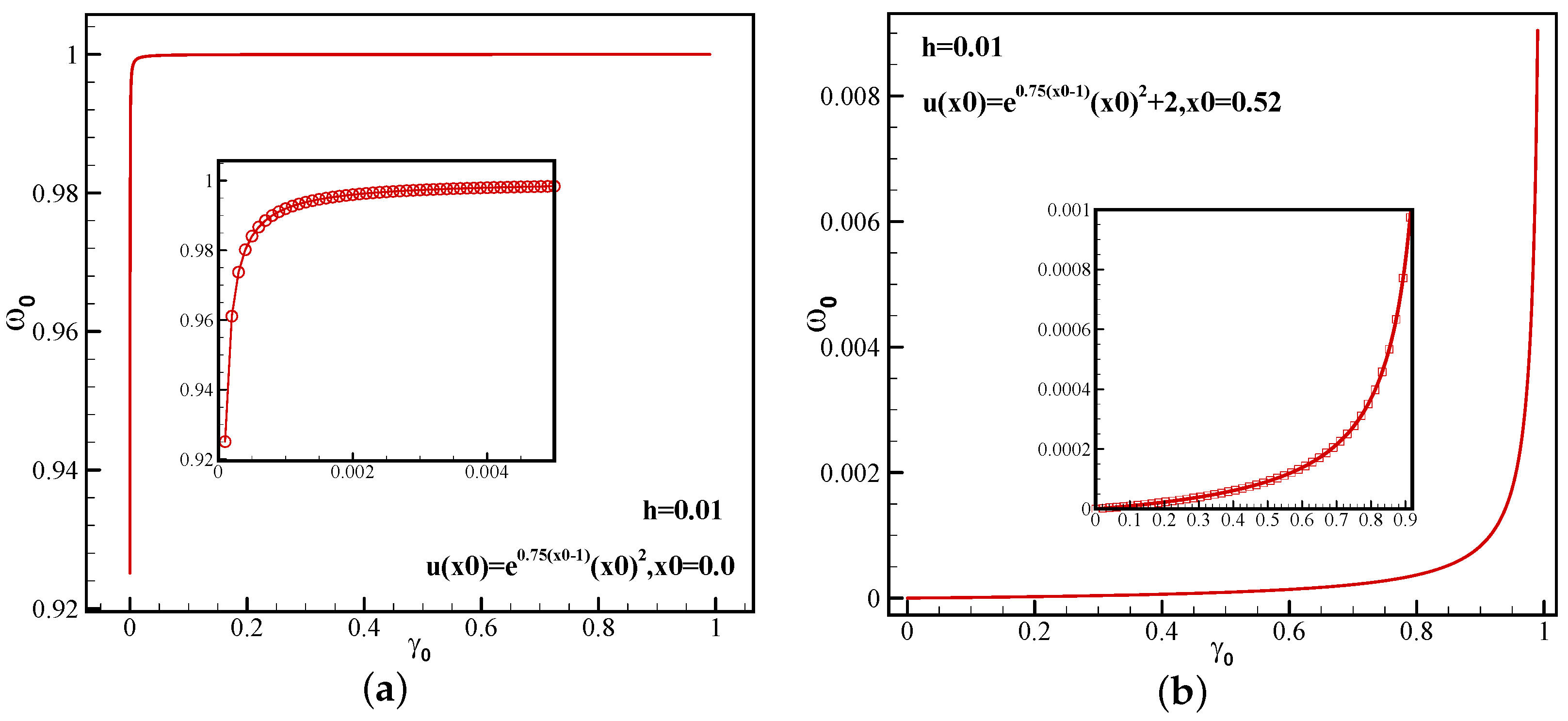
Figure 1.
The variation of nonlinear weight with linear weight for 5-point stencil: (a) first-order extreme point; (b) discontinuities.
Figure 1.
The variation of nonlinear weight with linear weight for 5-point stencil: (a) first-order extreme point; (b) discontinuities.
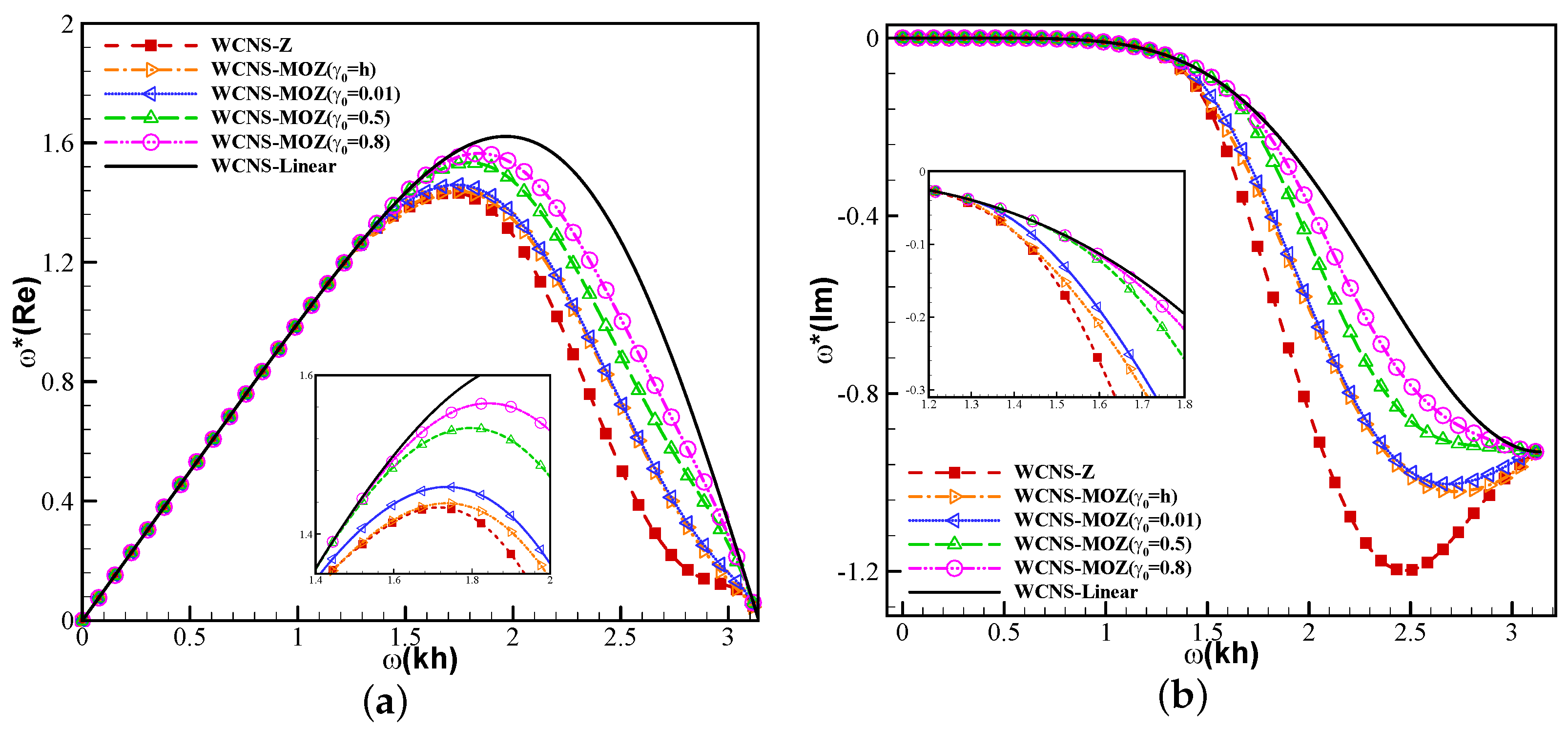
Figure 2.
Results of spectral characteristics of nonlinear weights using MOZ and Z: (a) real part; (b) imaginary part. (Red square symbol denotes the result based on Z weights; Yellow right triangle, blue left triangle, green top triangle, and purple circle have MOZ weights of , respectively; Solid lines indicate linear format).
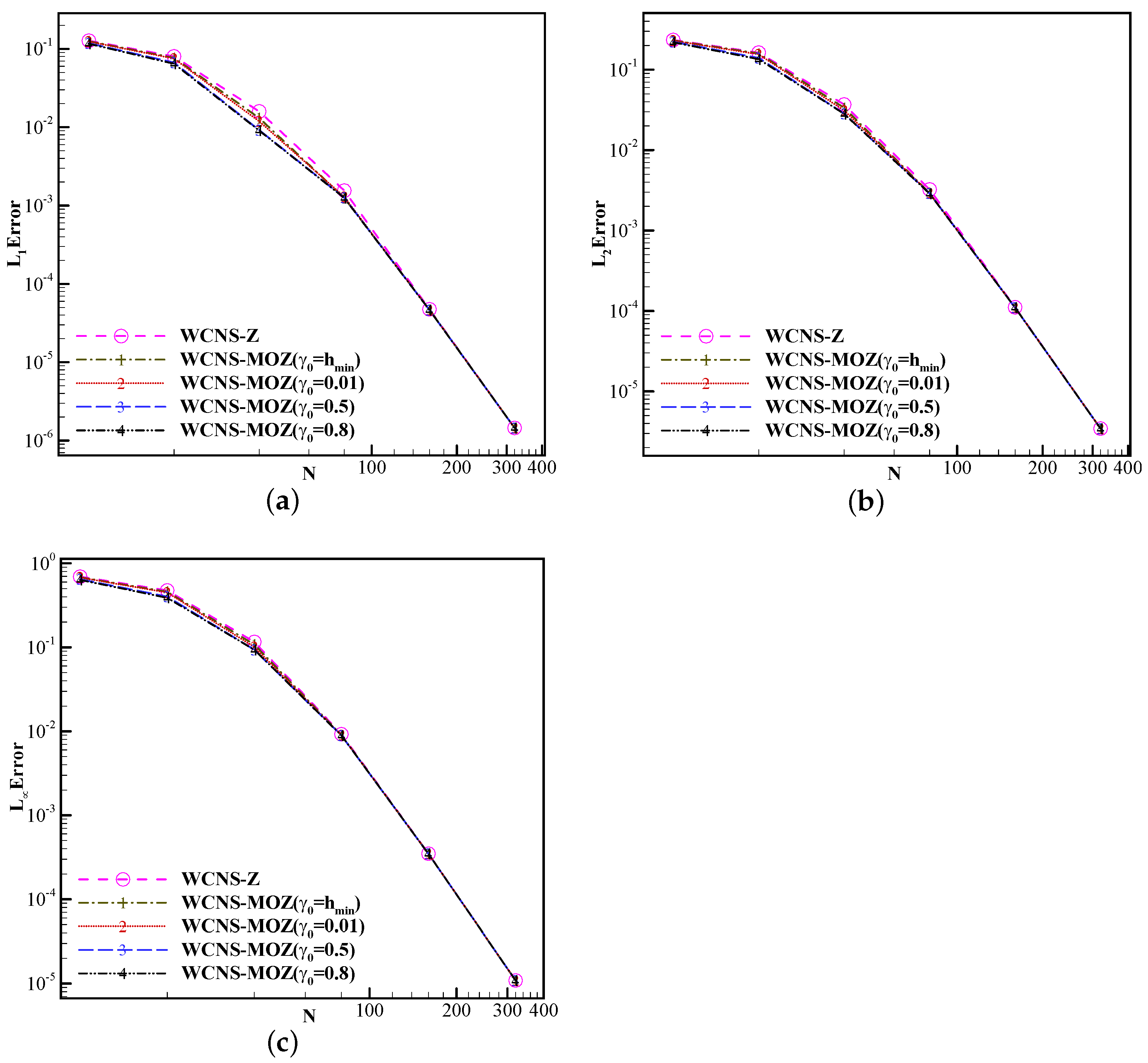
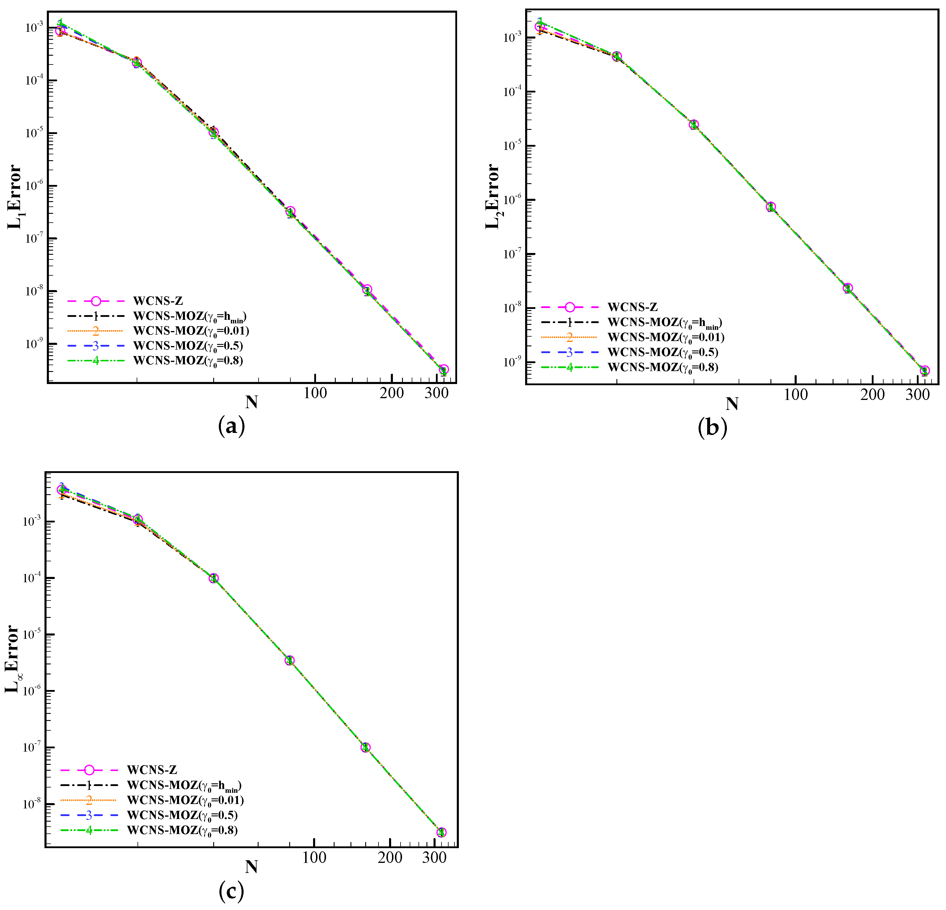
Figure 3.
Convergence orders of fifth-order schemes based on Z and MOZ weighting with different linear weights at for the case of based on the linear advection equation. (The horizontal axis represents the number of grid points (N) used in the calculation. The error of (a), (b), and (c) has already been provided in the previous text respectively. The circular symbol denotes the result of Z weighting; values of 1, 2, 3, and 4 denote the results of different linear weights of MOZ weighting).
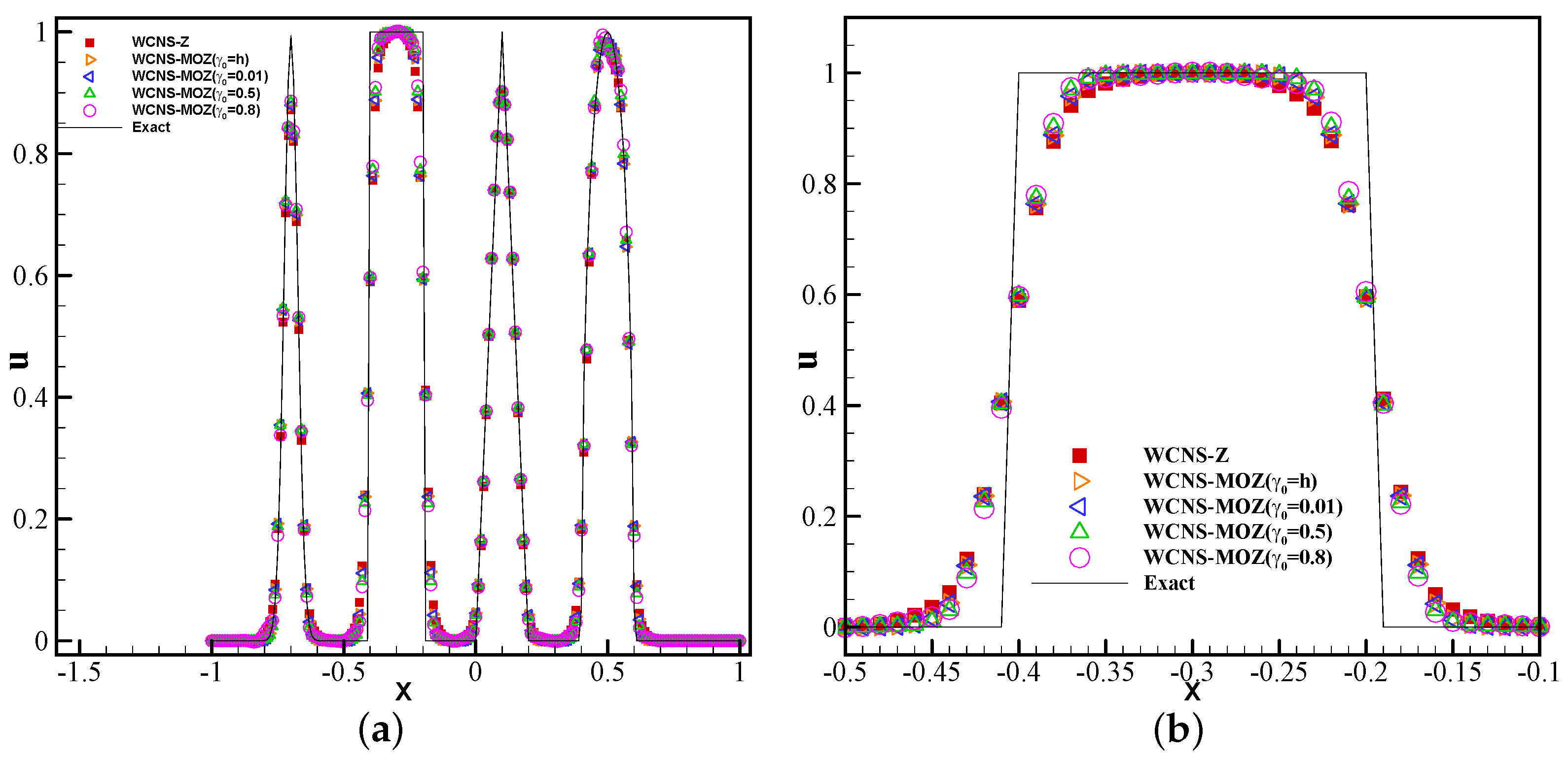
Figure 4.
Test of three types of nonlinear weights based on piecewise discontinuous solutions using 200 grid points at t = 8: (a) variable u; (b) variable u zoomed in. (Red square symbol denotes the result based on Z weighting; yellow right triangle, blue left triangle, green top triangle, and purple circle have MOZ weightings of , respectively; solid lines denotes the exact solution).
Figure 5.
Convergence orders of four nonlinear fifth-order schemes at of the one-dimensional inviscid Burgers’ equation with (The horizontal axis represents the number of grid points (N) used in the calculation. The error of (a), (b), and (c) has already been provided in the previous text respectively. The circular symbol denotes the result of Z weighting; values of 1, 2, 3, and 4 denote the results of different linear weights of MOZ weighting).
Figure 6.
The results of four nonlinear fifth-order schemes of the one-dimensional inviscid Burgers’ equation with at , grid N:100. (Red square symbol denotes the result based on Z weighting; yellow top triangle, blue right triangle, and green left triangle have MOZ weighting of , respectively; solid lines denote the exact solution.)
Figure 7.
Numerical and exact solutions of the Sod problem at t = 0.25 using 200 grid points: (a) density; (b) density zoomed in (red square symbol denotes Z weighting, blue upper triangle denotes MOZ weighting, and solid line denotes the exact solution).
Figure 7.
Numerical and exact solutions of the Sod problem at t = 0.25 using 200 grid points: (a) density; (b) density zoomed in (red square symbol denotes Z weighting, blue upper triangle denotes MOZ weighting, and solid line denotes the exact solution).
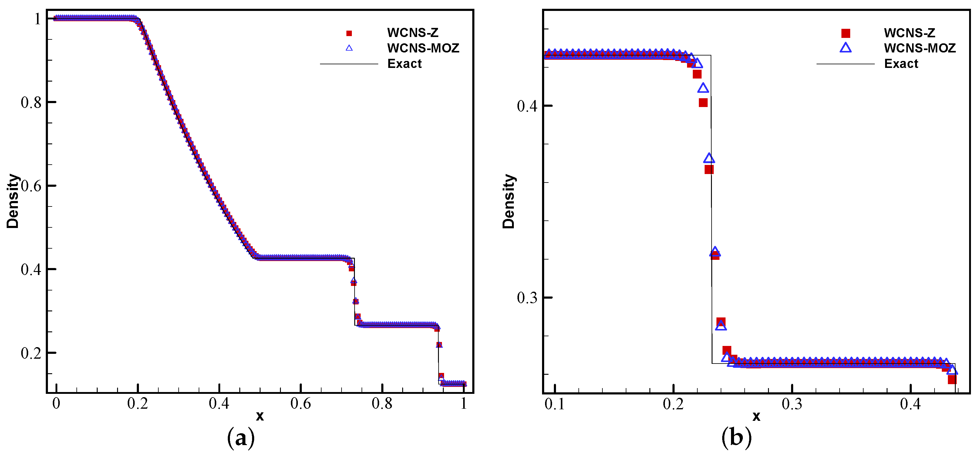
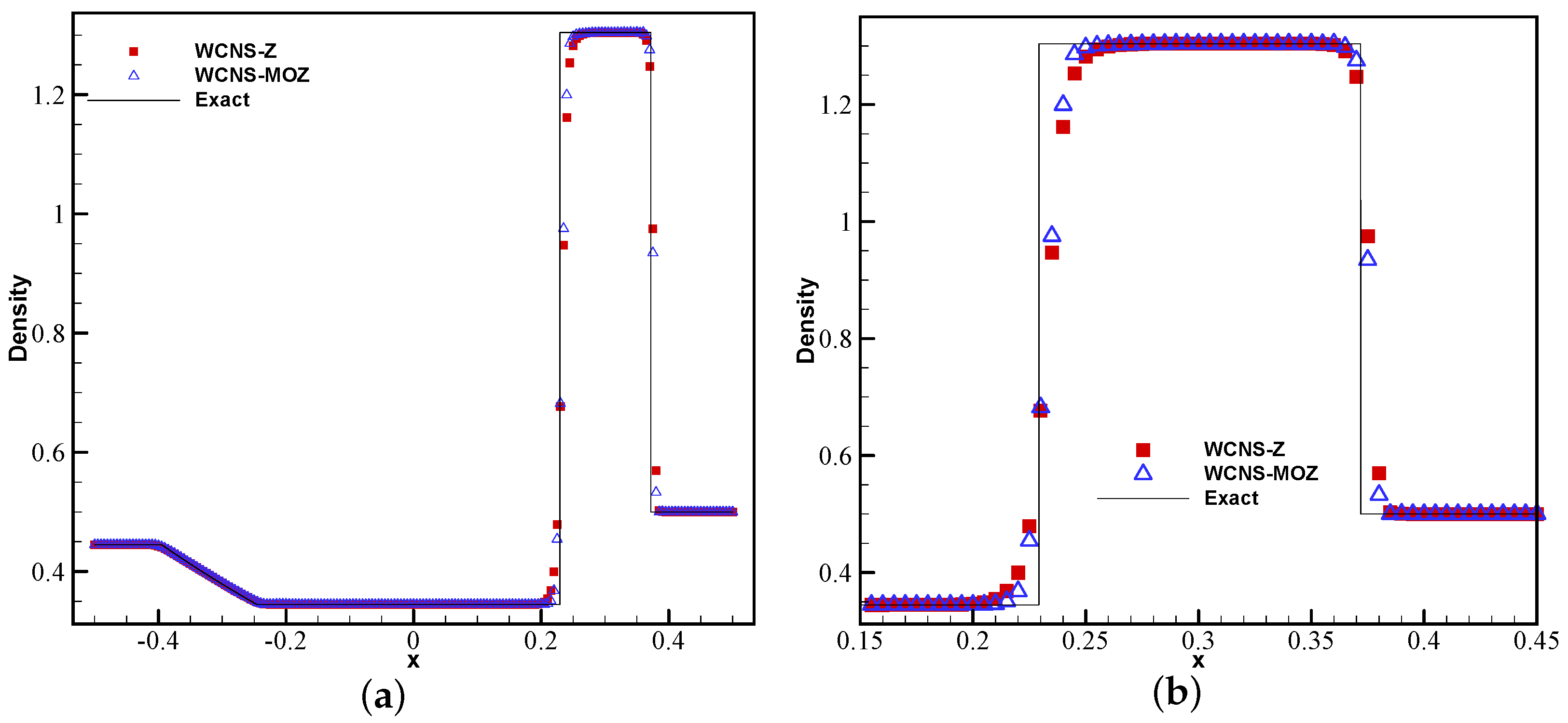
Figure 8.
Numerical and exact solutions of the Lax problem at t = 0.15 using 200 grid points: (a) density; (b) density zoom in (red square symbol denotes Z weighting, blue upper triangle denotes MOZ weighting, and solid line denotes the exact solution).
Figure 8.
Numerical and exact solutions of the Lax problem at t = 0.15 using 200 grid points: (a) density; (b) density zoom in (red square symbol denotes Z weighting, blue upper triangle denotes MOZ weighting, and solid line denotes the exact solution).
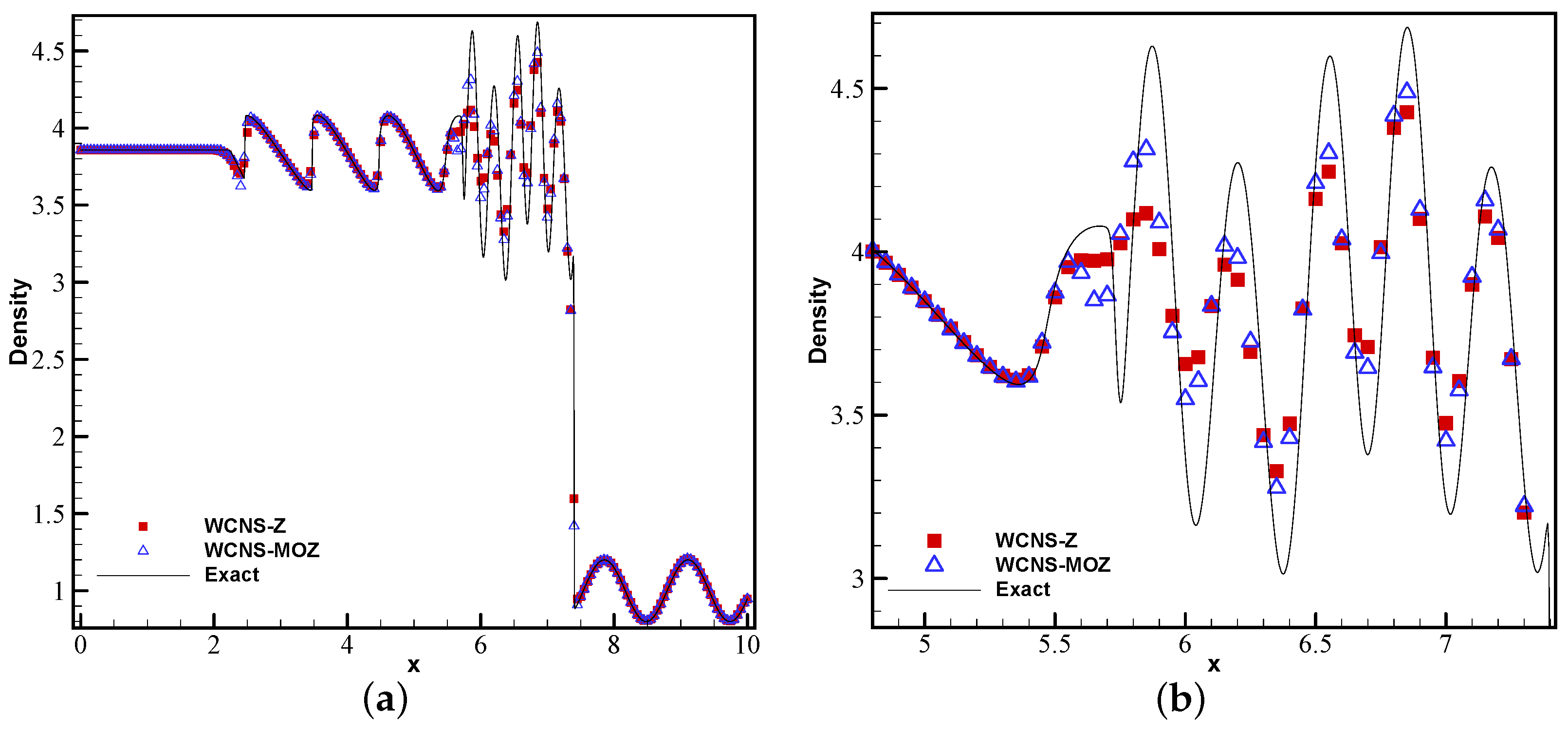
Figure 9.
Numerical and exact solutions of the Shu–Osher problem at t = 1.8 using 200 grid points: (a) density; (b) density zoom in (red square symbol denotes Z weighting, blue upper triangle denotes MOZ weighting, and solid line denotes the exact solution).
Figure 9.
Numerical and exact solutions of the Shu–Osher problem at t = 1.8 using 200 grid points: (a) density; (b) density zoom in (red square symbol denotes Z weighting, blue upper triangle denotes MOZ weighting, and solid line denotes the exact solution).
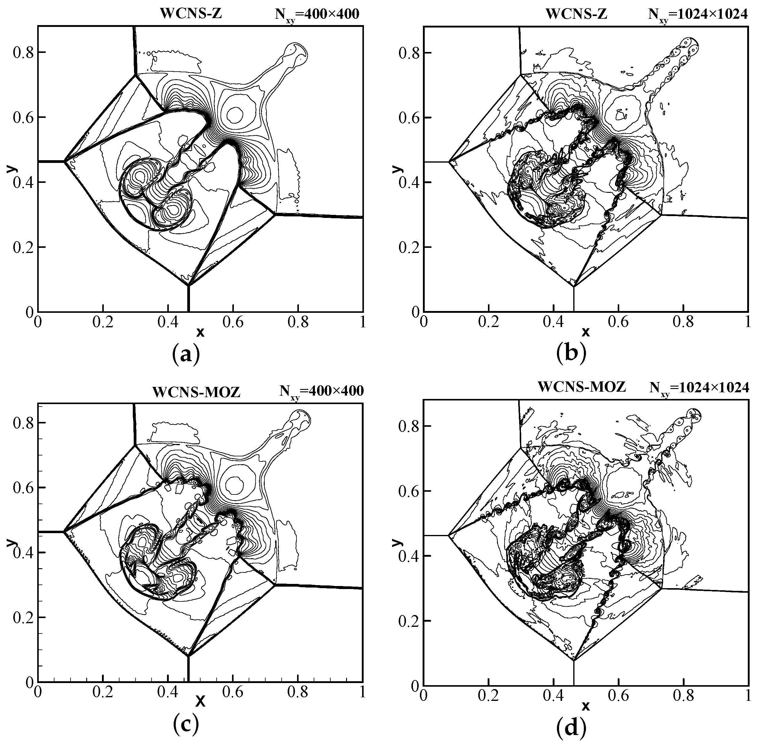
Figure 10.
The density contour of 2D-Lax–Liu–Riemannian problem at t = 0.8 using 400 × 400 and 1024 × 1024 grid points. CFL = 0.3. The figures use 30 density contour lines ranging from 0.1–1.8. (a,b) Z; (c,d) MOZ.
Figure 10.
The density contour of 2D-Lax–Liu–Riemannian problem at t = 0.8 using 400 × 400 and 1024 × 1024 grid points. CFL = 0.3. The figures use 30 density contour lines ranging from 0.1–1.8. (a,b) Z; (c,d) MOZ.
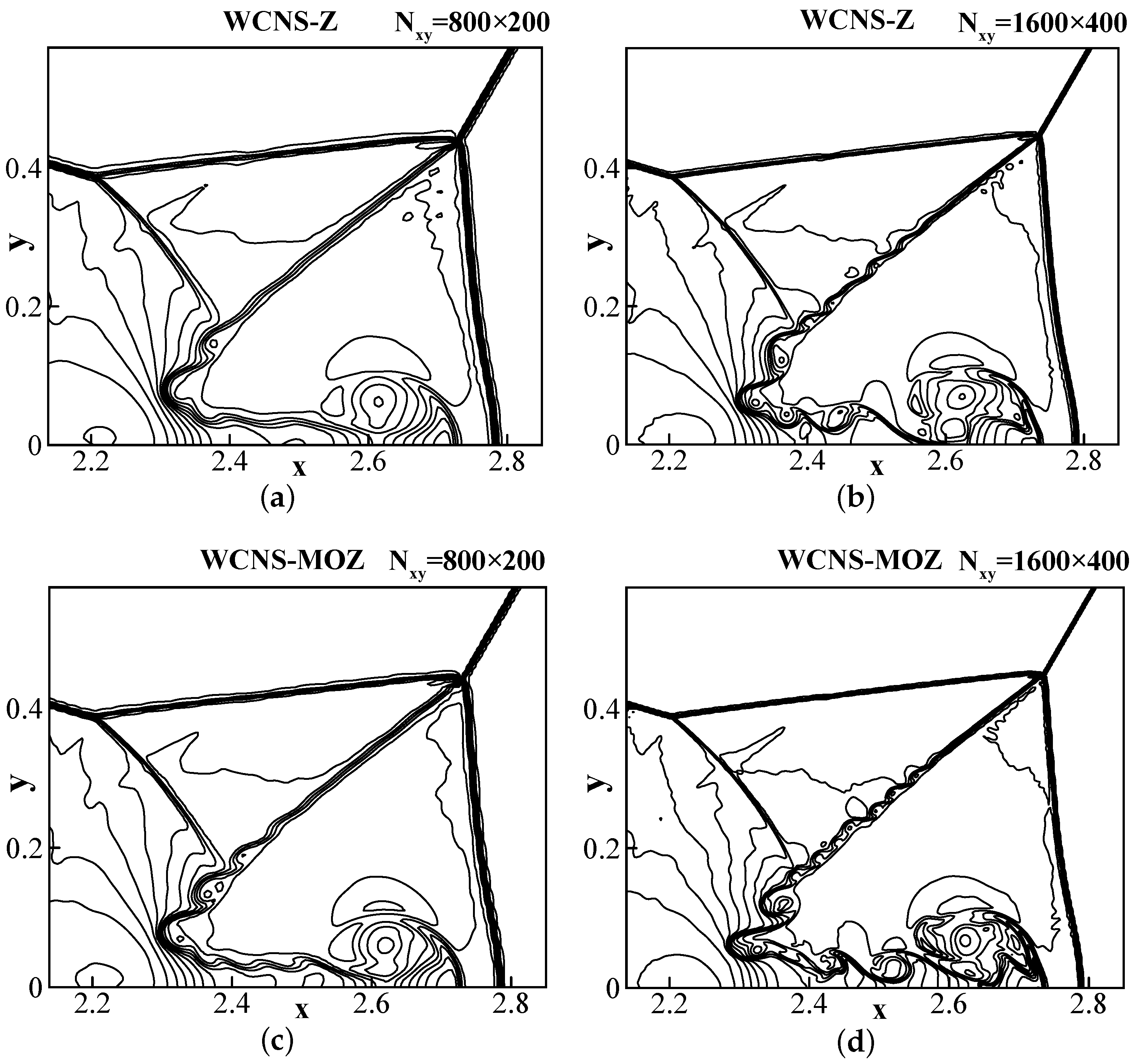
Figure 11.
The density contour of double Mach reflection problem at t = 0.2 using 800 × 200 and 1600 × 400 grid points. CFL = 0.3. The figures use 30 density contour lines ranging from 1.5–22.7. (a,b) Z; (c,d) MOZ.
Figure 11.
The density contour of double Mach reflection problem at t = 0.2 using 800 × 200 and 1600 × 400 grid points. CFL = 0.3. The figures use 30 density contour lines ranging from 1.5–22.7. (a,b) Z; (c,d) MOZ.
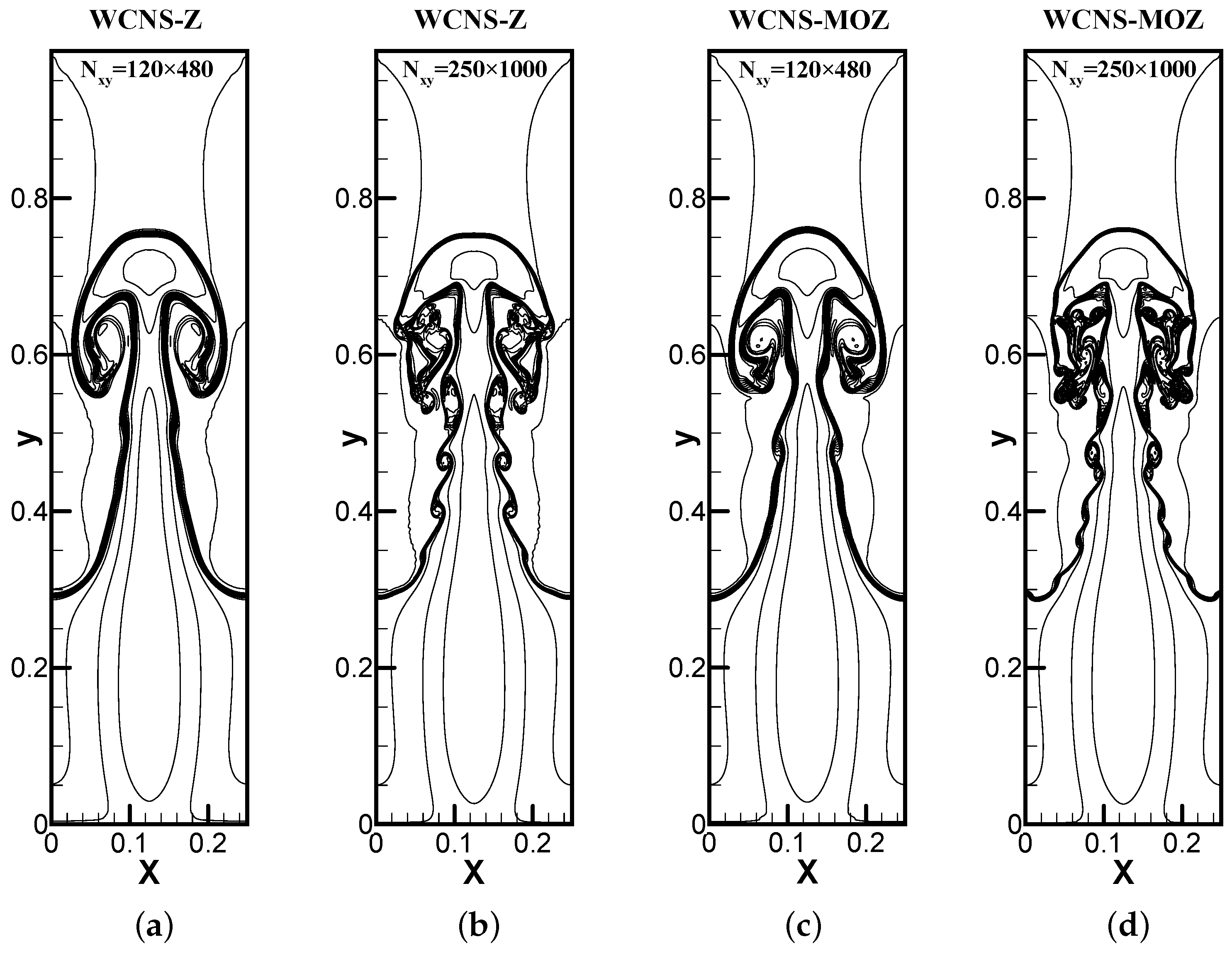
Figure 12.
The density contour of Rayleigh–Taylor instability problem at t = 1.95 using 120 × 480 and 250 × 1000 grid points. CFL = 0.3. The figures use 30 density contour lines ranging from 0.9–2.2. (a,b) Z; (c,d) MOZ.
Figure 12.
The density contour of Rayleigh–Taylor instability problem at t = 1.95 using 120 × 480 and 250 × 1000 grid points. CFL = 0.3. The figures use 30 density contour lines ranging from 0.9–2.2. (a,b) Z; (c,d) MOZ.
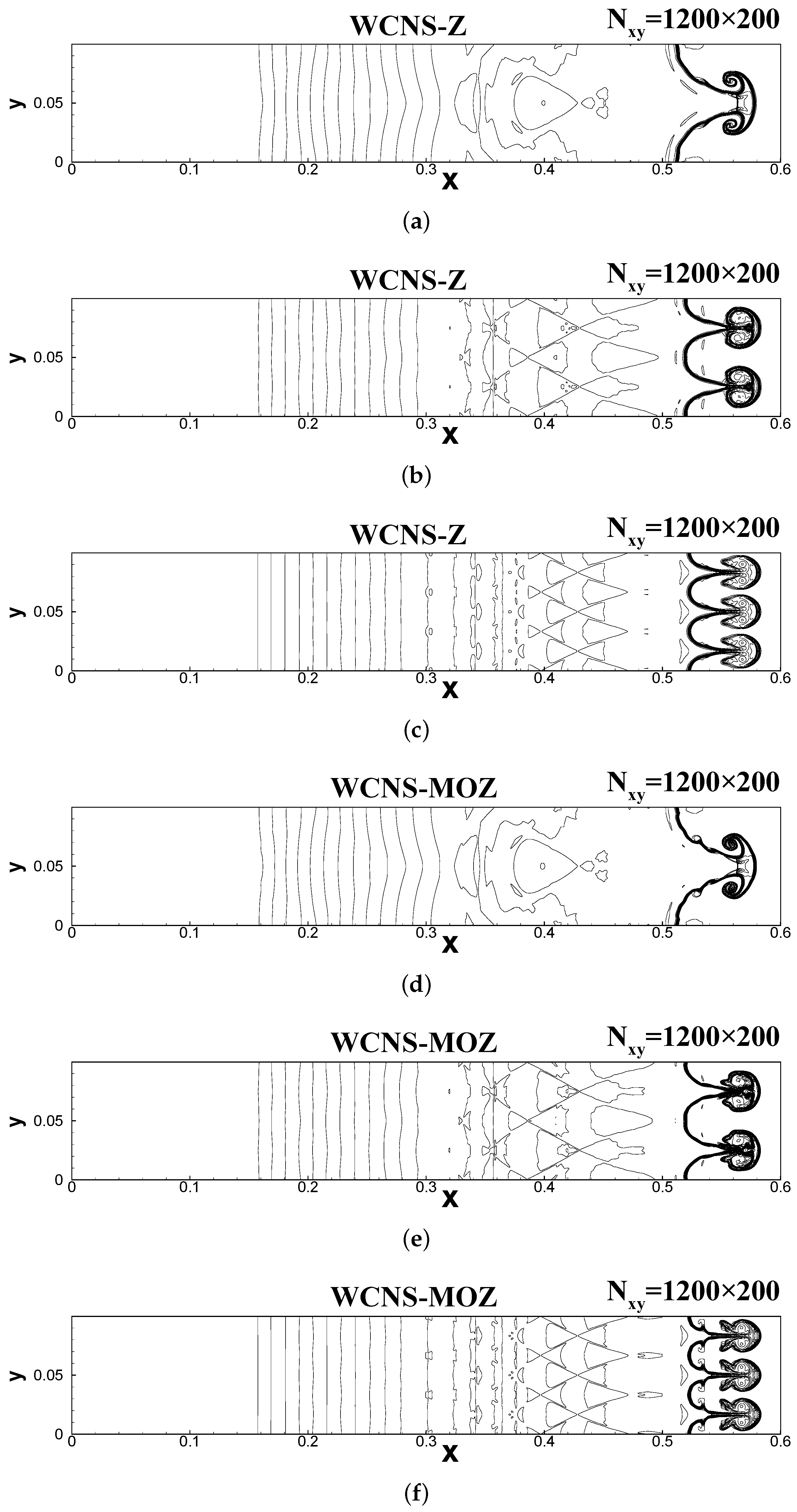
Figure 13.
The density contour of the Richtmyer–Meshkova instability problem at t = 0.16 using 1200 × 200 grid points. CFL = 0.3. The figures use 30 density contour lines ranging from 0.2–3.2. (a,c,e) Results for Z weighting for cases with n = 20, 40, and 60, respectively; similarly, (b,d,f) are the results for MOZ weighting for cases with n = 20, 40, and 60, respectively.
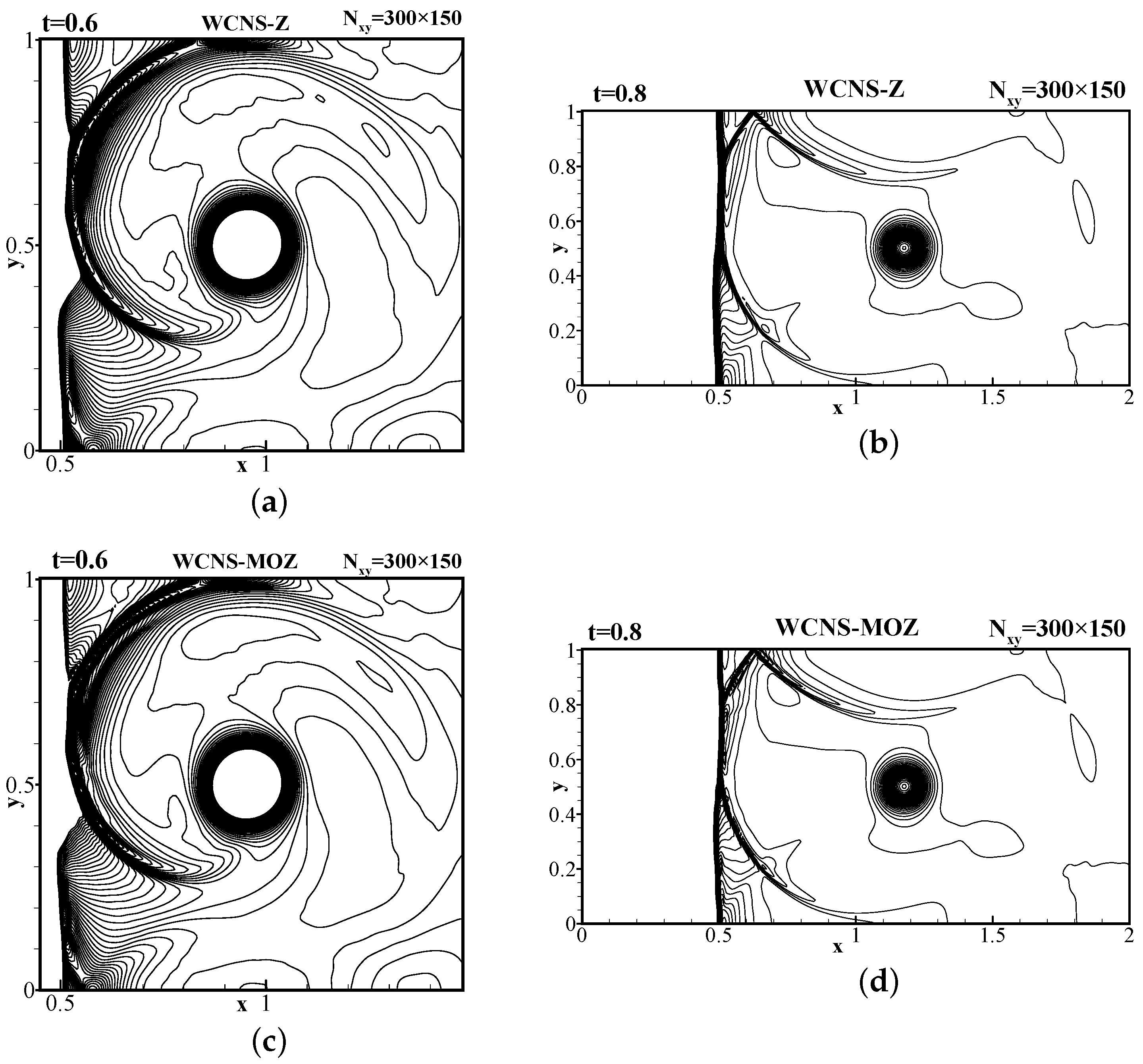
Figure 14.
Pressure contour lines of shock vortex interaction problem using 300 × 150 grid points. (a,b) Present the pressure distribution of Z weighting at t = 0.6 and t = 0.8, respectively; (c,d) present the pressure distribution of MOZ weighting at t = 0.6 and t = 0.8, respectively. There are 60 pressure contour lines ranging from 1.19∼13.7. CFL = 0.3.
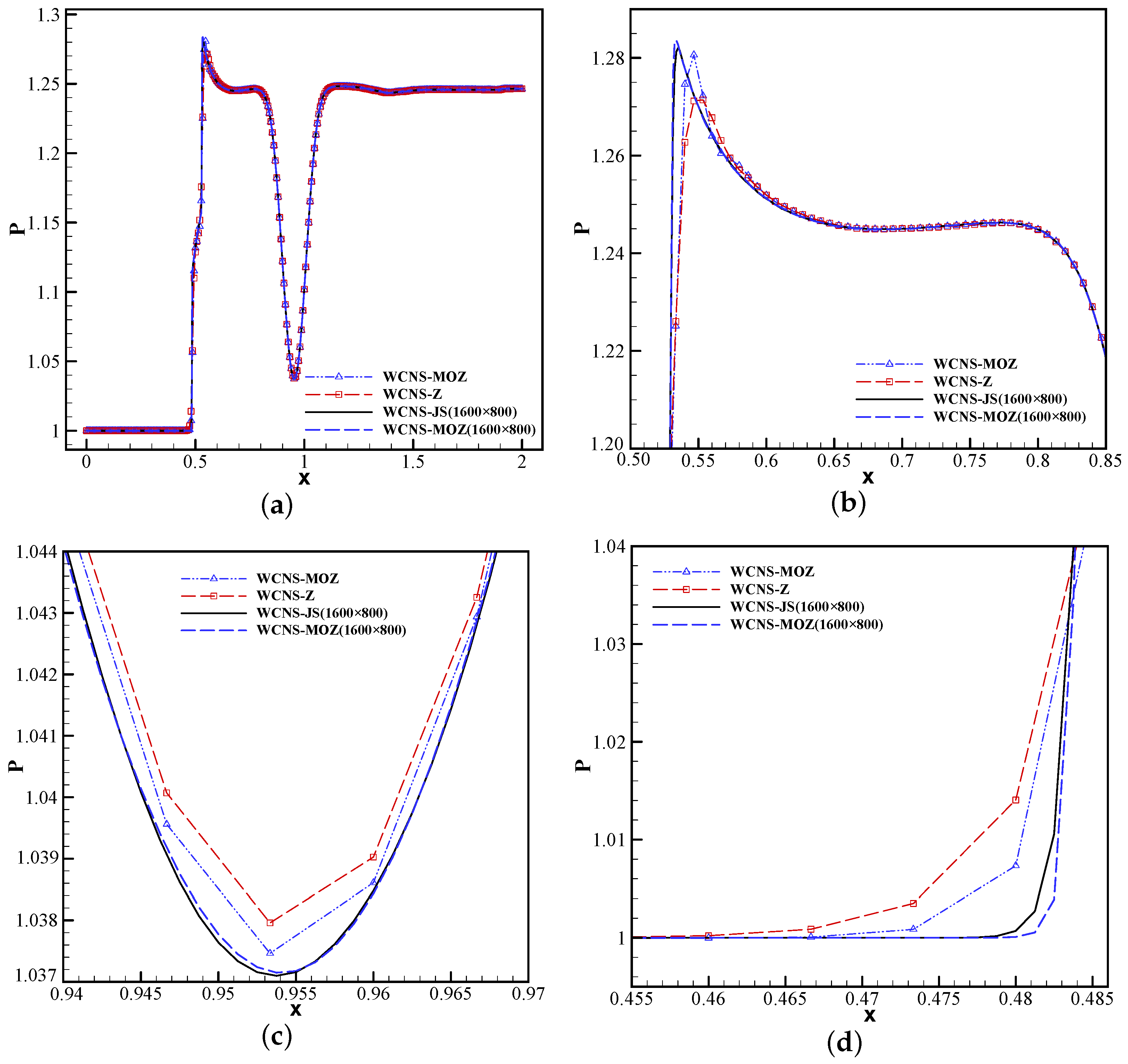
Figure 15.
Pressure distribution for the line y = 0.5 across the center of the vortex at t = 0.6 using 300 × 150 grid points. (a) Pressure distribution using different weights. (b)Pressure zoomed in for the post-shock position. (c) Pressure zoomed in near the center of the vortex. (d) Pressure zoomed in for the pre-shock position. The reference solution is calculated using JS weights and 1600 × 800 grid points. (The red square symbol denotes Z weighting, the blue upper triangle denotes MOZ weighting, the blue long dash line denotes MOZ weighting (1600 × 800 grid points), the black solid line denotes the reference solution.)
Table 1.
Errors and accuracy of nonlinear weighted interpolation method at first-order extreme point for the case for grids of .
Table 1.
Errors and accuracy of nonlinear weighted interpolation method at first-order extreme point for the case for grids of .
| | WCNS-Z | WCNS-MOZ
| WCNS-MOZ
| WCNS-MOZ
| WCNS-MOZ
|
| m | Error | Order | Error | Order | Error | Order | Error | Order | Error | Order |
| 0 | 1.37 × 10 | | 2.41 × 10 | | 7.62 × 10 | | 5.30 × 10 | | 5.28 × 10 | |
| 1 | 2.92 × 10 | 5.55 | 1.66 × 10 | 7.18 | 1.66 × 10 | 5.52 | 1.66 × 10 | 4.99 | 1.66 × 10 | 4.99 |
| 2 | 6.71 × 10 | 5.44 | 5.23 × 10 | 4.99 | 5.23 × 10 | 4.99 | 5.23 × 10 | 4.99 | 5.23 × 10 | 4.99 |
| 3 | 1.71 × 10 | 5.30 | 1.64 × 10 | 5.00 | 1.64 × 10 | 5.00 | 1.64 × 10 | 5.00 | 1.64 × 10 | 5.00 |
| 4 | 4.73 × 10 | 5.18 | 5.12 × 10 | 5.00 | 5.12 × 10 | 5.00 | 5.12 × 10 | 5.00 | 5.12 × 10 | 5.00 |
| 5 | 1.38 × 10 | 5.10 | 1.60 × 10 | 5.00 | 1.60 × 10 | 5.00 | 1.60 × 10 | 5.00 | 1.60 × 10 | 5.00 |
Table 2.
Errors and accuracy of nonlinear weighted interpolation method at second-order extreme point for the case for grids of .
Table 2.
Errors and accuracy of nonlinear weighted interpolation method at second-order extreme point for the case for grids of .
| | WCNS-Z | WCNS-MOZ
| WCNS-MOZ
| WCNS-MOZ
| WCNS-MOZ
|
| m | Error | Order | Error | Order | Error | Order | Error | Order | Error | Order |
| 0 | 7.50 × 10 | | 2.80 × 10 | | 2.80 × 10 | | 2.80 × 10 | | 2.80 × 10 | |
| 1 | 1.84 × 10 | 2.03 | 8.86 × 10 | 4.98 | 8.86 × 10 | 4.98 | 8.86 × 10 | 4.98 | 8.86 × 10 | 4.98 |
| 2 | 4.35 × 10 | 2.08 | 2.78 × 10 | 4.99 | 2.78 × 10 | 4.99 | 2.78 × 10 | 4.99 | 2.78 × 10 | 4.99 |
| 3 | 9.44 × 10 | 2.20 | 8.73 × 10 | 5.00 | 8.73 × 10 | 5.00 | 8.73 × 10 | 5.00 | 8.73 × 10 | 5.00 |
| 4 | 1.94 × 10 | 2.28 | 2.73 × 10 | 5.00 | 2.73 × 10 | 5.00 | 2.73 × 10 | 5.00 | 2.73 × 10 | 5.00 |
| 5 | 4.30 × 10 | 2.18 | 8.55 × 10 | 5.00 | 8.55 × 10 | 5.00 | 8.55 × 10 | 5.00 | 8.55 × 10 | 5.00 |
Table 3.
A comparison of CPU times obtained by solving the scalar equation with different nonlinear weights (the grid N is 1600).
Table 3.
A comparison of CPU times obtained by solving the scalar equation with different nonlinear weights (the grid N is 1600).
| Nonlinear Weights | JS | Z | MOZ |
| CPU time | 0.484 s | 0.516 s | 0.531 s |
| Time ratio | 1.000 | 1.066 | 1.097 |
Table 4.
For , , the error and order of Z weighting and different linear weights of MOZ weighting.
Table 4.
For , , the error and order of Z weighting and different linear weights of MOZ weighting.
| WCNS-MOZ |
| Grid Point Number | | | |
| Error | Order | Error | Order | Error | Order |
| 11 | 1.25 × 10 | | 2.31 × 10 | | 6.83 × 10 | |
| 21 | 7.69 × 10 | 0.70 | 1.59 × 10 | 0.54 | 4.59 × 10 | 0.57 |
| 41 | 1.31 × 10 | 2.55 | 3.35 × 10 | 2.25 | 1.08 × 10 | 2.08 |
| 81 | 1.25 × 10 | 3.39 | 2.90 × 10 | 3.53 | 9.02 × 10 | 3.59 |
| 161 | 4.68 × 10 | 4.75 | 1.10 × 10 | 4.71 | 3.47 × 10 | 4.70 |
| 321 | 1.45 × 10 | 5.01 | 3.44 × 10 | 5.00 | 1.09 × 10 | 5.00 |
| WCNS-MOZ |
| Grid Point Number | | | |
| Error | Order | Error | Order | Error | Order |
| 11 | 1.24 × 10 | | 2.30 × 10 | | 6.79 × 10 | |
| 21 | 7.50 × 10 | 0.73 | 1.55 × 10 | 0.57 | 4.49 × 10 | 0.60 |
| 41 | 1.19 × 10 | 2.65 | 3.11 × 10 | 2.32 | 1.01 × 10 | 2.16 |
| 81 | 1.29 × 10 | 3.21 | 2.92 × 10 | 3.41 | 8.97 × 10 | 3.49 |
| 161 | 4.65 × 10 | 4.80 | 1.10 × 10 | 4.73 | 3.47 × 10 | 4.69 |
| 321 | 1.45 × 10 | 5.01 | 3.44 × 10 | 5.00 | 1.09 × 10 | 5.00 |
| WCNS-MOZ |
| Grid Point Number | | | |
| Error | Order | Error | Order | Error | Order |
| 11 | 1.18 × 10 | | 2.22 × 10 | | 6.48 × 10 | |
| 21 | 6.68 × 10 | 0.82 | 1.40 × 10 | 0.67 | 4.02 × 10 | 0.69 |
| 41 | 9.17 × 10 | 2.86 | 2.83 × 10 | 2.30 | 9.36 × 10 | 2.10 |
| 81 | 1.26 × 10 | 2.86 | 2.89 × 10 | 3.29 | 8.93 × 10 | 3.39 |
| 161 | 4.64 × 10 | 4.76 | 1.10 × 10 | 4.71 | 3.47 × 10 | 4.69 |
| 321 | 1.45 × 10 | 5.00 | 3.44 × 10 | 5.00 | 1.09 × 10 | 5.00 |
| WCNS-MOZ |
| Grid Point Number | | | |
| Error | Order | Error | Order | Error | Order |
| 11 | 1.16 × 10 | | 2.19 × 10 | | 6.36 × 10 | |
| 21 | 6.45 × 10 | 0.85 | 1.35 × 10 | 0.70 | 3.89 × 10 | 0.71 |
| 41 | 9.06 × 10 | 2.83 | 2.82 × 10 | 2.26 | 9.35 × 10 | 2.06 |
| 81 | 1.25 × 10 | 2.86 | 2.88 × 10 | 3.29 | 8.93 × 10 | 3.39 |
| 161 | 4.64 × 10 | 4.75 | 1.10 × 10 | 4.71 | 3.47 × 10 | 4.69 |
| 321 | 1.45 × 10 | 5.00 | 3.44 × 10 | 5.00 | 1.09 × 10 | 5.00 |
| WCNS-Z |
| Grid Point Number | | | |
| Error | Order | Error | Order | Error | Order |
| 11 | 1.27 × 10 | | 2.34 × 10 | | 6.95 × 10 | |
| 21 | 8.01 × 10 | 0.66 | 1.63 × 10 | 0.52 | 4.77 × 10 | 0.55 |
| 41 | 1.59 × 10 | 2.34 | 3.69 × 10 | 2.15 | 1.16 × 10 | 2.04 |
| 81 | 1.55 × 10 | 3.35 | 3.24 × 10 | 3.51 | 9.24 × 10 | 3.64 |
| 161 | 4.74 × 10 | 5.04 | 1.11 × 10 | 4.87 | 3.49 × 10 | 4.73 |
| 321 | 1.45 × 10 | 5.03 | 3.45 × 10 | 5.01 | 1.09 × 10 | 5.00 |
Table 5.
For , , the error and order of Z weighting and different linear weights of MOZ weighting.
Table 5.
For , , the error and order of Z weighting and different linear weights of MOZ weighting.
| WCNS-MOZ |
| Grid Point Number | | | |
| Error | Order | Error | Order | Error | Order |
| 11 | 8.23 × 10 | | 1.36 × 10 | | 2.95 × 10 | |
| 21 | 2.33 × 10 | 1.82 | 4.34 × 10 | 1.65 | 9.74 × 10 | 1.60 |
| 41 | 1.14 × 10 | 4.36 | 2.50 × 10 | 4.12 | 9.88 × 10 | 3.30 |
| 81 | 3.11 × 10 | 5.19 | 7.37 × 10 | 5.08 | 3.47 × 10 | 4.83 |
| 161 | 9.79 × 10 | 4.99 | 2.27 × 10 | 5.02 | 9.96 × 10 | 5.12 |
| 321 | 2.95 × 10 | 5.05 | 6.60 × 10 | 5.11 | 3.15 × 10 | 4.98 |
| WCNS-MOZ |
| Grid Point Number | | | |
| Error | Order | Error | Order | Error | Order |
| 11 | 8.35 × 10 | | 1.42 × 10 | | 3.13 × 10 | |
| 21 | 2.33 × 10 | 1.84 | 4.48 × 10 | 1.66 | 1.02 × 10 | 1.61 |
| 41 | 1.03 × 10 | 4.50 | 2.45 × 10 | 4.19 | 9.88 × 10 | 3.37 |
| 81 | 2.97 × 10 | 5.12 | 7.32 × 10 | 5.06 | 3.47 × 10 | 4.83 |
| 161 | 9.79 × 10 | 4.93 | 2.27 × 10 | 5.01 | 9.96 × 10 | 5.12 |
| 321 | 2.95 × 10 | 5.05 | 6.60 × 10 | 5.11 | 3.15 × 10 | 4.98 |
| WCNS-MOZ |
| Grid Point Number | | | |
| Error | Order | Error | Order | Error | Order |
| 11 | 1.13 × 10 | | 1.91 × 10 | | 4.10 × 10 | |
| 21 | 2.08 × 10 | 2.44 | 4.58 × 10 | 2.06 | 1.14 × 10 | 1.85 |
| 41 | 9.54 × 10 | 4.45 | 2.92 × 10 | 4.24 | 9.88 × 10 | 3.52 |
| 81 | 2.96 × 10 | 5.01 | 7.31 × 10 | 5.05 | 3.47 × 10 | 4.83 |
| 161 | 9.79 × 10 | 4.92 | 2.27 × 10 | 5.01 | 9.96 × 10 | 5.12 |
| 321 | 2.95 × 10 | 5.05 | 6.60 × 10 | 5.11 | 3.15 × 10 | 4.98 |
| WCNS-MOZ |
| Grid Point Number | | | |
| Error | Order | Error | Order | Error | Order |
| 11 | 1.23 × 10 | | 1.95 × 10 | | 3.82 × 10 | |
| 21 | 2.09 × 10 | 2.56 | 4.56 × 10 | 2.10 | 1.14 × 10 | 1.74 |
| 41 | 9.54 × 10 | 4.45 | 2.42 × 10 | 4.23 | 9.88 × 10 | 3.53 |
| 81 | 2.96 × 10 | 5.01 | 7.31 × 10 | 5.05 | 3.47 × 10 | 4.83 |
| 161 | 9.79 × 10 | 4.92 | 2.27 × 10 | 5.01 | 9.96 × 10 | 5.12 |
| 321 | 2.95 × 10 | 5.05 | 6.60 × 10 | 5.11 | 3.15 × 10 | 4.98 |
| WCNS-Z |
| Grid Point Number | | | |
| Error | Order | Error | Order | Error | Order |
| 11 | 8.80 × 10 | | 1.60 × 10 | | 3.66 × 10 | |
| 21 | 2.18 × 10 | 2.02 | 4.49 × 10 | 1.83 | 1.08 × 10 | 1.76 |
| 41 | 1.04 × 10 | 4.39 | 2.46 × 10 | 4.19 | 9.89 × 10 | 3.45 |
| 81 | 3.31 × 10 | 4.97 | 7.46 × 10 | 5.04 | 3.47 × 10 | 4.83 |
| 161 | 1.08 × 10 | 4.93 | 2.35 × 10 | 4.98 | 9.96 × 10 | 5.12 |
| 321 | 3.29 × 10 | 5.04 | 7.01 × 10 | 5.07 | 3.15 × 10 | 4.98 |
Table 6.
Errors and convergence orders based on JS, Z, and MOZ weights for two-dimensional Euler vortex simulation, at .
Table 6.
Errors and convergence orders based on JS, Z, and MOZ weights for two-dimensional Euler vortex simulation, at .
| WCNS-JS |
| Grid Point Number | | | |
| Error | Order | Order | Error | Order | Error |
| 41 | 8.88 × 10 | | 3.19 × 10 | | 1.06 × 10 | |
| 81 | 1.16 × 10 | 2.94 | 8.05 × 10 | 1.99 | 2.94 × 10 | 0.44 |
| 161 | 1.33 × 10 | 3.13 | 1.06 × 10 | 2.92 | 2.78 × 10 | 3.40 |
| 321 | 8.41 × 10 | 3.98 | 6.84 × 10 | 3.95 | 1.88 × 10 | 3.89 |
| 641 | 2.46 × 10 | 5.09 | 2.13 × 10 | 5.00 | 8.64 × 10 | 4.44 |
| WCNS-Z |
| Grid Point Number | | | |
| Error | Order | Order | Error | Order | Error |
| 41 | 5.48 × 10 | | 1.89 × 10 | | 9.26 × 10 | |
| 81 | 9.01 × 10 | 2.61 | 6.74 × 10 | 1.49 | 2.34 × 10 | 0.31 |
| 161 | 1.11 × 10 | 3.02 | 9.26 × 10 | 2.86 | 2.39 × 10 | 3.29 |
| 321 | 5.60 × 10 | 4.31 | 5.47 × 10 | 4.08 | 1.88 × 10 | 3.67 |
| 641 | 9.79 × 10 | 5.84 | 1.08 × 10 | 5.66 | 4.95 × 10 | 5.25 |
| WCNS-MOZ |
| Grid Point Number | | | |
| Error | Order | Order | Error | Order | Error |
| 41 | 3.09 × 10 | | 1.21 × 10 | | 2.51 × 10 | |
| 81 | 3.52 × 10 | 3.13 | 2.37 × 10 | 2.36 | 5.77 × 10 | 1.62 |
| 161 | 2.93 × 10 | 3.58 | 2.51 × 10 | 3.24 | 5.60 × 10 | 3.37 |
| 321 | 7.17 × 10 | 5.35 | 7.27 × 10 | 5.11 | 2.61 × 10 | 4.43 |
| 641 | 7.81 × 10 | 6.52 | 4.23 × 10 | 7.43 | 1.21 × 10 | 7.75 |


