On Casimir and Helmholtz Fluctuation-Induced Forces in Micro- and Nano-Systems: Survey of Some Basic Results

Abstract

Fluctuations are omnipresent; they exist in any matter, due either to its quantum nature or to its nonzero temperature. In the current review, we briefly cover the quantum electrodynamic Casimir (QED) force as well as the critical Casimir (CC) and Helmholtz (HF) forces. In the QED case, the medium is usually a vacuum and the massless excitations are photons, while in the CC and HF cases the medium is usually a critical or correlated fluid and the fluctuations of the order parameter are the cause of the force between the macroscopic or mesoscopic bodies immersed in it. We discuss the importance of the presented results for nanotechnology, especially for devising and assembling micro- or nano-scale systems. Several important problems for nanotechnology following from the currently available experimental findings are spelled out, and possible strategies for overcoming them are sketched. Regarding the example of HF, we explicitly demonstrate that when a given integral quantity characterizing the fluid is conserved, it has an essential influence on the behavior of the corresponding fluctuation-induced force.

1. Introduction

Let us consider two flat half-spaces A and B separated by a gap with thickness L filled with a medium C which fluctuates with the characteristic energy E of the pertinent fluctuations. If the fluctuations decay with the distance slowly enough, say, algebraically (which takes place if the corresponding excitations are massless), then changes in the fluctuations due to A will be felt by B (and vice versa), leading to a force between A and B. Such a force bears the natural name of fluctuation-induced force (FIF) $F^{\Vert }$, where ‖ simply reminds us about the geometry we are discussing. The L-dependence of $F^{\Vert }$ can be easily determined on dimensional grounds; as for any force, we have $F^{\Vert }\propto Energy/Length\propto E/L$. In the considered geometry, it is natural to consider the normalized force per unit area $A\sim L^2$, then obtain it for the corresponding pressure $p^{\Vert }\sim E/L^3$. Taking into account that in quantum systems $E\sim h{\nu }_0\sim hc/L$, where ${\nu }_0$ is some characteristic frequency of the quantum system, while in classical systems $E\sim k_{B}T$, we obtain

$$p_{\mathrm{quantum}}^{\Vert }\sim hc/L^4,p_{\mathrm{classical}}^{\Vert }\sim k_{B}T/L^3.$$

(1)

Naturally, the classical result also holds if, in a given quantum system, $k_{B}T\gg h{\nu }_0$; in Equation (1), h is Planck’s constant, c is the speed of light, $k_B$ is Boltzmann’s constant, and T is the temperature of the system. Equation (1) reflects essential parts of the QED Casimir, critical Casimir (CCE), and (as we will see) Helmholtz force effects. Of course, the precise behavior of $p_{\mathrm{quantum}}^{\Vert }$ and $p_{\mathrm{classical}}^{\Vert }$, e.g., the corresponding pre-factors cannot be obtained in such a simple way, and the efforts of many scientists have been dedicated to figuring out the corresponding details. Below, we briefly comment on this topic.

The current most prominent example of a fluctuation-induced force involves the force due to quantum or thermal fluctuations of the electromagnetic field, leading to the so-called QED Casimir effect, named after the Dutch physicist H.B. Casimir. Casimir first realized that in the case of two perfectly-conducting, uncharged, and smooth plates parallel to each other in vacuum, at $T=0$ (see Figure 1) these fluctuations lead to an attractive force between them [1]. In other words, Casimir demonstrated that the boundary conditions imposed by two plates (denoted in the following by $\parallel$) on the spectrum of the quantum mechanical zero-point fluctuations of the electromagnetic field lead to the above remarkable mechanical effect involving the appearance of a long-range attractive force between the plates. More precisely, for the corresponding pressure he obtained

$$F_{\mathrm{Cas}}^{\Vert }\left(L\right)=-\frac{{\pi }^2}{240}\frac{\hslash c}{L^4}=-1.3\times {10}^{-3}\frac{1}{{(L/\mu m)}^4}\frac{\mathrm{N}}{{\mathrm{m}}^2}.$$

(2)

Intuitively, this pressure can be viewed as the difference in radiation pressure of virtual photons outside and inside the pore formed by the two plates, which results in an attractive force $F_{\mathrm{Cas}}^{\Vert }$ between them [2]. The accepted terminology terms the negative force as the attractive one. In order to derive Equation (2), Casimir calculated the derivative with respect to L of the energy difference $\delta E$ [1]: (i) when A and B are at infinite distance, and (ii) when they are at a distance L from each other (see below for more details).

There is a vast amount of literature concerning research on the quantum Casimir effect. Here, we only mention the review articles in [3,4,5,6,7,8,9,10,11,12,13,14,15,16,17,18,19,20,21,22,23,24,25,26,27,28,29,30,31,32,33,34,35,36,37,38], involving recent studies of the dynamical Casimir effect (in which actual photons can be created if a single mechanical mirror undergoes accelerated motion in vacuum) [39,40,41,42,43,44,45,46] and studies of the effects which emerge in systems out of thermodynamic equilibrium (in which the material bodies are characterized by different temperatures) [47,48,49,50,51,52,53]. Currently, the QED Casimir effect is a popular subject of research. The Casimir and Casimir-like effects are objects of studies in quantum electrodynamics, quantum chromodynamics, cosmology, condensed matter physics, and biology, with some elements of it present in nanotechnology as well. Investigations devoted to the topic are currently being performed on many fronts, including research ranging from attempts to unify the four fundamental forces of nature [6,11,12] to rather more practical issues such as the design and the performance of micro- and nanoscale machines [16,22,23,54,55]. Readers interested in these topics can consult the existing reviews cited above.

Looking at the problem from the historical perspective, in 1978, thirty years after Casimir, Fisher and De Gennes [56] showed that a very similar effect exists in fluids. As the main setup for discussing the CCE, we can envisage two material bodies, $\left(1\right)$ and $\left(2\right)$, immersed in a fluid (see Figure 2). They exert an effective force $F^{(1,2)}$ on each other, which is mediated by the fluid; this includes, inter alia, the direct interaction between material bodies $\left(1\right)$ and $\left(2\right)$. If the thermodynamic state of the fluid is far away from a bulk phase transition at $T=T_c$, this force varies slowly and smoothly as function of the temperature T. Upon approaching $T_c$ of a continuous phase transition, $F^{(1,2)}$ acquires a contribution $F_{\mathrm{Cas}}^{(1,2)}$ due to the critical fluctuations of the confined fluid. This singular contribution encompasses both the distortion of the local (eventually) nonzero order parameter (due to the finite distance between $\left(1\right)$ and $\left(2\right)$) and the fluctuations of the order parameter. The singular contribution $F_{\mathrm{Cas}}^{(1,2)}$ follows by subtracting the smooth background contribution (after extrapolating it to the neighborhood of $T_c$) from $F^{(1,2)}$. Upon the above construction, in the disordered phase, $F^{(1,2)}$ and $F_{\mathrm{Cas}}^{(1,2)}$ vanish in the limit of increasing separation between the bodies $\left(1\right)$ and $\left(2\right)$. Taking into account that in the d-dimensional space the surface $A\propto L^{d-1}$ and that the energy of the fluctuations $E\propto k_{B}T$, it can be concluded that $F_{\mathrm{Cas}}^{\Vert }\propto k_{B}T/L^d$ for the thermodynamic Casimir effect near the critical point of the system. For a $(d=3)$-dimensional system, we can write the force at the critical point $T=T_c$ in the following form:

$$F_{\mathrm{Cas}}^{\Vert \left(\tau \right)}(T=T_c,L)\simeq 8.1\times {10}^{-3}{\displaystyle \frac{{\Delta }^{\left(\tau \right)}(d=3)}{{(L/\mu \mathrm{m})}^3}}{\displaystyle \frac{T_c}{T_{\mathrm{roon}}}}{\displaystyle \frac{\mathrm{N}}{{\mathrm{m}}^2}}$$

(3)

where $T_{\mathrm{room}}$ = 20 °C (293.15 K). The above equation is in a full agreement with Equation (1). In order to calculate $F_{\mathrm{Cas}}^{\Vert \left(\tau \right)}$, it is normally necessary to determine the finite size-dependent part of the properly normalized difference between the energy of the infinite and finite systems, similar to the QED case (see below). Here, ${\Delta }^{\left(\tau \right)}$ is the so-called Casimir amplitude, which depends on the bulk and surface universality classes (see below) of the system and the applied boundary conditions$\tau$. For most systems and boundary conditions, ${\Delta }^{\left(\tau \right)}\left(d\right)=\mathcal{O}\left(1\right)$; thus, when $T_c\simeq T_{\mathrm{room}}$, both forces (quantum and thermodynamic) can be of the same order of magnitude, i.e., they can both be essential, measurable, and obviously significant at or below the micrometer length scale. We stress here that ${\Delta }^{\left(\tau \right)}\left(d\right)$ can be both positive and negative, i.e., $F_{\mathrm{Cas}}^{\Vert \left(\tau \right)}(T,L)$ can be both attractive and repulsive. Recently, a review of the exact results available for the CCE has been published [57]; overviews of different aspects of this effect can be found in [57,58,59,60,61].

The above arguments for two semi-spaces A and B separated by a fluid C can be easily extended for bodies A and B of general shape immersed in a fluid, say, two spheres, a sphere and a semi-space (plane surface), etc. In the general case, it is the confinement of a fluctuating field by the surfaces of the material bodies which causes FIF acting on the confining surfaces of these bodies. In the current review, we do not consider such geometries, and simply refer interested readers to the existing reviews on QED and the critical Casimir effects for further details.

When considering the FIF between A and B immersed in a fluctuating medium C, it is always supposed that the constituents of C can enter and leave the region between objects A and B. There are, however, two important subcases. In the first, C is in contact with a reservoir, i.e., its constituents can enter and leave the part of the space occupied by A and B. In this case, we can speaks of the bona fide Casimir force. In the second case, the system itself is bounded such that some integral quantity characterizing the amount of material in C is conserved, say, the total mass or the integral over the volume of the system or the order parameter. In this case, we can speak about the recently introduced (see [62]) and not yet well studied Helmholtz force. Currently, there are only a few articles devoted to these forces [62,63,64,65]. Note that in HF case we are again near a critical point of the medium C. As it turns out, however, the HF has a behavior distinctly different from that of the Casimir force. Because the study of Helmholtz forces is a relatively new field of research, in the current review we devote special attention to it and its behavior, both as a function of the temperature and of an external ordering field characterizing the medium C. We show this via exact results for the one-dimensional Ising model in a fixed-order parameter M ensemble. We stress that in customarily considered applications involving, say, the equilibrium Ising model with respect to binary alloys or binary liquids, if one insists on full rigor, the case with a fixed order parameter must be addressed. It is interesting to note that the HF in the case of periodic boundary conditions shows behavior similar to that appearing in certain versions of the big bang theory, e.g., strong repulsion at high temperatures transitioning to moderate attraction for intermediate values of the temperature and then back to repulsion, albeit much more weakly than during the initial period of highest temperature.

We stress that the definition and existence of Helmholtz force (see Section 4) is by no means limited to the Ising chain, and can be addressed in principle in any model of interest.

In addition, we note that the issue of the ensemble dependence of fluctuation-induced forces pertinent to the ensemble has yet to be studied.

The remainder of this review is structured as follows. First, in Section 2 we briefly consider the QED Casimir effect. Section 3 introduces details of the critical and thermodynamic Casimir effects, while Section 4 presents the definition of the Helmholtz force. Results for this force using the example of Ising chains with periodic, antiperiodic, and Dirichlet boundary conditions as well as with a defect bond are summarized in Section 5. Finally, concluding remarks about the FIF, including their role in nanotechnology, are presented in Section 6.

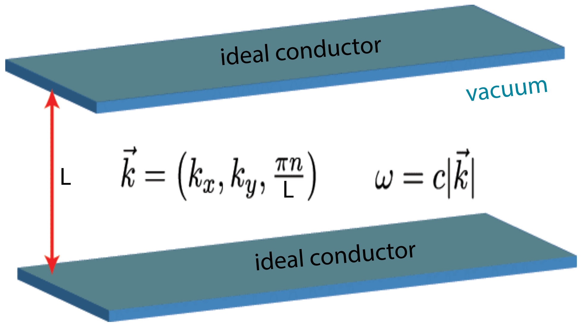
2. The QED Casimir Effect

As already alluded to in the introduction, the confinement of a fluctuating field generates effective forces on the confining surfaces, which nowadays are termed FIF.

The relationship in Equation (2) can be derived by considering the change of the structure of the electromagnetic modes between the two plates as compared with those in free space after assigning the zero-point energy $\frac{1}{2}\hslash \omega$ to each electromagnetic mode, i.e., photon of frequency $\omega$. We emphasize that, in the absence of charges on the plates, the mean value of the electric field $\mathbf{E}$ and the magnetic field $\mathbf{B}$ vanishes, i.e.,

$$\langle \mathbf{E}\rangle =0\mathrm{and}\langle \mathbf{B}\rangle =0,$$

(4)

while

$$\langle {\mathbf{E}}^2\rangle \ne 0\mathrm{and}\langle {\mathbf{B}}^2\rangle \ne 0,$$

(5)

meaning that the expectation value of the energy due to the electromagnetic field, i.e., $\langle \mathcal{H}\rangle$ with

$$\mathcal{H}=\int \left[\frac{1}{2}{\epsilon }_0{\mathbf{E}}^2\left(\mathbf{r}\right)+\frac{1}{2{\mu }_0}{\mathbf{B}}^2\left(\mathbf{r}\right)\right]d^3\mathbf{r},$$

(6)

is nonzero. In fact, according to quantum field theory, the energy of the electromagnetic field in the vacuum state in free space is infinitely large, and all physically relevant energies are measured relative to the energy of the vacuum. When the two (in the above sense ideal) parallel smooth metal plates are placed against each other in free space, the tangential component of the electric field and the normal component of the magnetic induction must vanish at the plate surfaces. As a result, not all zero-point oscillations occur. Subtracting the energy of the vacuum energy in free space from that of the allowed modes, after taking the derivative with respect to L, we obtain the result reported in Equation (2). In more detail, focusing on a single component of the electric field, which vanishes at the surface of the metal (this discussion can be easily extended to include all vector components), the simultaneous presence of two parallel walls restricts the allowed wave vector $k_{\perp }$ of the field in the direction normal to the plates, meaning that the field itself vanishes at both walls (Dirichlet boundary conditions). If we instead impose no restriction on the wave vector $k_{\parallel }$ parallel to the plates, which are assumed to have a large lateral extension with a transverse area A and to be separated by a distance L, then we have $k_{\perp }=\pi n/L$ with $n=0,1,2,\cdots$, and the energy $\mathcal{E}$ contained within the confined space takes the form

$$\mathcal{E}=\sum _{\mathbf{k}}\frac{1}{2}\hslash \omega \left(\mathbf{k}\right),$$

(7)

where the sum runs over all allowed values of $\mathbf{k}=(k_{\parallel },k_{\perp })$ and where $\omega \left(\mathbf{k}\right)\equiv {\omega }_k=c\left|\mathbf{k}\right|=c\sqrt{k_{\parallel }^2+k_{\perp }^2}$ (with $\left|\mathbf{k}\right|=k$) is the frequency of the mode with wave vector $\mathbf{k}$. As it stands, the sum in Equation (7) diverges due to the fact that $|{\omega }_k|$ grows as k increases and because the sum lacks any ultraviolet cutoff, i.e., k is allowed to grow unboundedly. In this context, we are actually interested in the energy of the modes which can be “contained” by the metallic cavity, as they are the only ones affected by the presence of the cavity itself. At sufficiently high frequencies, the cavity becomes transparent to the electromagnetic field. Note that within the assumptions made when deriving Equation (2), no materials-dependent properties enter the picture; thus, the force depends only on the Planck constant ℏ and the speed of light in vacuum c as well as on the geometry of the pore (characterized here by L). In addition, the force does not depend on the electric charge e, implying that, for the present conditions of the phenomenon, the coupling between the electromagnetic field and the matter is unimportant, as is any other interaction.

In the aftermath of [1], there has been an intense theoretical effort to describe the force beyond the case of ideal plates by considering the actual dielectric properties of the two plates and the medium in between [17,66,67,68,69,70,71,72,73,74,75,76]. Specifically, the groundbreaking results of Lifshitz et al. [66,77], who developed a unified theory of the van der Waals and the Casimir forces, must be mentioned. It should be noted that, when discussing the quantum Casimir effect, the retarded van der Waals interactions are often called Casimir interactions; however, we retain the notion of retarded van der Waals interactions when discussing the thermodynamic Casimir effect in order to avoid confusion of these forces with the critical Casimir force, which we discuss later.

Lifshitz et al. studied the case of two materials acting as walls, described by frequency-dependent dielectric permittivities ${\epsilon }^{\left(n\right)}\left(\omega \right),n=1,2$, separated by a third material characterized by ${\epsilon }^{\left(0\right)}\left(\omega \right)$. It turns out that in the limit of small separations (still large compared with molecular scales), the Casimir force approaches the more familiar van der Waals force [17,78]. This more realistic description provides specific predictions which are amenable to high-precision measurements. The corresponding expressions for the force are also quite instructive in that they allows for prediction of how the material properties of the substances involved have to be tuned in order to modify the strength (and even the sign) of the force. According to Lifshitz, in order to calculate the Casimir pressure for a set of three dielectric materials, it is necessary to know their permittivities along the imaginary frequency axis. As experimental data for the complex permittivity

$$\epsilon \left(\omega \right)={\epsilon }^{\prime }\left(\omega \right)+i{\epsilon }^{″}\left(\omega \right),$$

(8)

where ${\epsilon }^{\prime },{\epsilon }^{″}\in \mathbb{R}$, exist only for real frequencies, the permittivity along the imaginary frequency axis has to be determined from the Kramers–Kronig relation (see, e.g., [79]):

$$\epsilon \left(i\xi \right)=1+\frac{2}{\pi }{\int }_0^{\infty }\frac{x{\epsilon }^{″}\left(x\right)}{x^2+{\xi }^2}dx.$$

(9)

From the Lifshitz theory, it can be inferred [78] that it is possible to observe Casimir repulsion in the film geometry if the two half-spaces (1) and (2) forming the plates and confining the film (0) exhibit permittivities which fulfill the relationship

$${\epsilon }^{\left(2\right)}\left(i\xi \right)<{\epsilon }^{\left(0\right)}\left(i\xi \right)<{\epsilon }^{\left(1\right)}\left(i\xi \right).$$

(10)

Experimentally, repulsion occurs if the inequality in Equation (10) holds over a sufficiently wide frequency range. Actually, this is a widespread phenomenon shared by all substrate–fluid systems which show complete wetting, such as in the old experiment by Sabisky and Anderson [80]. Accordingly, Casimir repulsion is a common feature [81]. In fact, it has been already observed; see, e.g., [82].

A standard approximation for obtaining the force between two bodies of nontrivial shape is the so-called Derjaguin approximation (DA) [83]. The DA term is used in colloidal science (see, e.g., [84] and p. 34 in [85]), while it is known as proximity force approximation in studies of the QED Casimir effect (see, e.g., p. 97 in [17]). The main idea behind the DA is that it is possible to relate the knowledge of the interaction force/potential between two parallel plates with that between two gently curved colloidal particles when the separation between them is much smaller than the geometrical characteristics of the particles in question. More specifically, the DA states that in $d=3$, the interaction force $F^{R_1,R_2}\left(L\right)$ between two spherical particles with radii $R_1$ and $R_2$ placed at a distance $L\ll R_1,R_2$ is provided by

$$F_{\mathrm{DA}}^{R_1,R_2}\left(L\right)=2\pi R_{\mathrm{eff}}{\int }_L^{\infty }{f}_{\mathcal{A}}^{\Vert }\left(z\right)\mathrm{d}z,$$

(11)

where $R_{\mathrm{eff}}^{-1}=R_1^{-1}+R_2^{-1}$ is an effective radius and $f_{\mathcal{A}}^{\Vert }$ is the force per unit area between parallel plates. When a sphere with radius $R_1\equiv R$ interacts with a plate, we have $R_2=\infty$. in which case (11) is still valid with $R_{\mathrm{eff}}=R$.

An improvement and generalization of the DA called the “surface integration approach” (SIA) has been proposed in [86]. It has been used there to study van der Waals interactions between objects of arbitrary shape and a plate of arbitrary thickness. It delivers exact results if the interactions involved can be described by pair potentials. The main advantage of this approach over the DA is that one is no longer bound by the restriction that the interacting objects must be much closer to each other than their characteristic sizes. The main result is that for the force acting between a $3\mathrm{d}$ object (say a colloid particle) $B\equiv \left\{\right(x,y,z),(x,y,z)\in B\}$ of general shape $S(x,y)=z$ and a flat surface bounded by the $(x,y)$—plane of a Cartesian coordinate system, we have

$$\begin{array}{c}\hfill F_{\mathrm{SIA}}^{B,|}\left(L\right)={\int }_{A_S^{\mathrm{to}}}\int f_{\mathcal{A}}^{\Vert }\left[\mathrm{S}(x,y)\right]\mathrm{d}x\mathrm{d}y-{\int }_{A_S^{\mathrm{away}}}\int f_{\mathcal{A}}^{\Vert }\left[\mathrm{S}(x,y)\right]\mathrm{d}x\mathrm{d}y,\end{array}$$

(12)

where $A_S$ is the projection of the surface S of the particle over the $(x,y)-$ plane, with $A_S=A_S^{\mathrm{to}}\bigcup A_S^{\mathrm{away}}$. Equation (12) has a very simple and intuitive meaning: in order to determine the force acting on the particle, it is necessary to subtract from the contributions stemming from surface regions $A_S^{\mathrm{to}}$ that “face towards” the projection plane those from regions $A_S^{\mathrm{away}}$ that “face away” from it, where $A_S^{\mathrm{to}}$ and $A_S^{\mathrm{away}}$ are the projections of the corresponding parts of the surface of the body on the $(x,y)$—plane. It is clear that when taking into account only the contributions over $A_S^{\mathrm{to}}$, we obtain expression very similar to those of DA. In this case, the two expressions differ only in the fact that (12) takes into account that the force on a given point of the S is along the normal to the surface at that point, while the standard DA does not take this into account. Recall that (12) provides exact results for the interaction under the assumption that the constituents of the body interact via pair potentials. This is, strictly speaking, not the case of the force in QED Casimir, i.e., Equation (12) is still an approximation. It is, however, clear that under mechanical equilibrium of the colloid in the fluid, the force is indeed along the normal to the surface at the point of the surface where it acts. Thus, it is possible to obtain a reasonably good approximation of the effect of this force by keeping only the integration over parts of the surface of the body that faces the plane. It should be noted that the importance of the SIA approach has been already recognized and used; see, e.g., [87,88,89,90,91,92]. For the QED Casimir force, such a generalization has been derived on the solid basis of quantum field theory in the framework of scattering approaches (see, e.g., [93,94]). This approach is widely used in making comparisons between theory and measurements of the QED Casimir force in sphere–plate geometries (see, e.g., [95]).

3. The Critical and Thermodynamic Casimir Effects

As explained above, the spatial restriction on the fluctuations of the order parameter describing a continuous phase transition of a many-body system leads to the so-called critical Casimir effect [56]. Then, the interactions in the system are mediated not by photons, as in the case of the electromagnetic field, but by different types of massless excitations. In the case that the critical point has a quantum origin, and instead of temperature certain quantum parameters govern the fluctuations in the system, we speak of the quantum critical Casimir effect [59,96]. In addition, systems such as liquid ⁴He and liquid crystals, i.e., so-called correlated fluids, exhibit gapless excitations called Goldstone modes [8,97,98,99]. These fluctuations also lead to long-ranged forces between the boundaries of the systems, although such systems are thermodynamically positioned below their respective critical points. For these cases, we speak of the noncritical Casimir effect, or more generally the thermodynamic Casimir effect. We shall use the latter notion as a general one that encompasses all cases in which the Casimir effect is due to the fluctuations of a certain order parameter.

The critical Casimir effect depends on the parameters describing the thermodynamic state of the critical medium, such as the temperature and an externally applied field (e.g., pressure, excess chemical potential, magnetic field), as well as on the distance L between $\left(1\right)$ and $\left(2\right)$; that is, the observed phenomenon is a finite size effect. Therefore, if L increases the effect, the magnitude of the associated force decreases and eventually vanishes.

Any thermodynamic system which is of finite extent in at least one spatial direction is called a finite-size system. The corresponding modification of its phase behavior compared with that of the bulk is described by finite-size scaling theory [59,100,101]. Because of the deep interconnection between the theory of the thermodynamic Casimir effect and finite-size scaling theory, we recall some basic facts concerning finite-size scaling theory which are relevant for studying the thermodynamic Casimir effect. We start by recollecting some basic properties of critical phenomena in bulk systems. In the vicinity of the bulk critical point $(T_c,h=0)$ governed by the temperature T and some external field h, the bulk correlation length of the order parameter $\xi$ becomes large and theoretically diverges: ${\xi }_t^{+}\equiv \xi (T\to T_c^{+},h=0)\simeq {\xi }_0^{+}{t}^{-\nu }$, $t=(T-T_c)/T_c$ and ${\xi }_h\equiv \xi (T=T_c,h\to 0)\simeq {\xi }_{0,h}{|h/\left(k_B{T}_c\right)|}^{-\nu /\Delta }$, where $\nu$ and $\Delta$ are the usual critical exponents and ${\xi }_0^{+}$ and ${\xi }_{0,h}$ are the corresponding nonuniversal amplitudes of the correlation length along the t and h axes. If, in a finite system, $\xi$ becomes comparable to L, the thermodynamic functions describing its behavior depend on the ratio $L/\xi$ and take scaling forms provided by finite-size scaling theory. Further information of the phase transitions and related physical and mathematical problems can be found in [59,100,101] and in the set of articles on the topic cited therein.

Crucial by its implications for systems with continuous phase transitions is the so-called universality hypothesis. It was initially formulated by Kadanoff [102]. According to this hypothesis, “all (continuous) phase transition problems can be divided into a small number of different classes depending upon the dimensionality of the system and the symmetries of the ordered state. Within each class, all phase transitions have identical behavior in the critical region; only the names of thermodynamic variables are changed”. All such systems are then part of the same universality class. For example, we have the Ising universality class characterized by breaking of the ${\mathbb{Z}}_2$ symmetry of the original effective Hamiltonian for the scalar order parameter, the $XY$ universality class with a two-component order parameter and a disordered phase with $O\left(2\right)$ symmetry, and the Heisenberg universality class characterized by a vectorial order parameter with an $O\left(3\right)$ symmetry. Any of these bulk universality classes is accompanied by a set of surface universality classes which depend on the behavior of the order parameter near and at a surface(s) of the semi-infinite or finite system. For a film geometry, the accumulated experimental and theoretical evidence supports the statement that the Casimir force is attractive when the boundary conditions on either plate are the same or similar and is repulsive when they essentially differ from each other. For the case of a one-component fluid, the latter means that one of the surfaces adsorbs the liquid phase of the fluid while the other prefers the vapor phase. This rule, which connects the type of boundary condition with the type of the force, seems to be violated if competing interactions are present in the system. Recently, it has been established that, under periodic boundary conditions, an Ising chain with a defect bound can have a Casimir force which changes sign as a function of T provided that an antiferromagnetic bond is present within the otherwise ferromagnetic bonds of the chain [65].

In the remainder of the current section, we discuss the thermodynamic Casimir effect in a system with a ${\infty }^{d-1}\times L$ film geometry. We envisage a system exposed to a temperature T and an external ordering field h that couples to its order parameter, i.e., density, concentration difference, magnetization M, etc. We imagine as examples a simple fluid system at its liquid–vapor critical point, a magnet at the phase transition from paramagnetic to ferromagnetic state, and a binary liquid mixture or binary alloy with phases A and B near its consolute temperature point. Letting $(T=T_c,h=0)$ be this bulk critical point in the $(T,h)$ plane, we consider only the case of an one-dimensional order parameter $\varphi \in \mathbb{R}$. The thermodynamic Casimir force $F_{\mathrm{Cas}}(T,h,L)$ in such a system is the excess pressure over the bulk pressure, and acts on the boundaries of the finite system due to the finite size of the system, i.e.,

$$F_{\mathrm{Cas}}(T,h,L)=P_L(T,h)-P_b(T,h),$$

(13)

where $P_L$ is the pressure in the finite system while $P_b$ is that in the infinite system. Note that the above definition is actually equivalent to another commonly used definition [58,59,103]:

$$F_{\mathrm{Cas}}(T,h,L)\equiv -\frac{\partial {\omega }_{\mathrm{ex}}(T,h,L)}{\partial L}=-\frac{\partial {\omega }_L(T,h,L)}{\partial L}-P_b$$

(14)

where ${\omega }_{\mathrm{ex}}={\omega }_L-L{\omega }_b$ is the excess grand potential per unit area, ${\omega }_L$ is the grand canonical potential of the finite system, again per unit area, and ${\omega }_b$ is the density of the grand potential for the infinite system. The equivalence between the definitions in Equations (13) and (14) comes from the observation that ${\omega }_b=-P_b$ and that for a finite system with surface area A and thickness L it is the case that ${\omega }_L={lim}_{A\to \infty }{\Omega }_L/A$ with $-\partial {\omega }_L(T,h,L)/\partial L=P_L$. When $F_{\mathrm{Cas}}(\tau ,h,L)<0$, the excess pressure of the system will be inward; this corresponds to an attraction of the surfaces of the system towards each other, and conversely to a repulsion if $F_{\mathrm{Cas}}(\tau ,h,L)>0$. Then, for a system positioned near its critical point, the finite-size scaling theory [58,59,100,101,104,105,106] predicts for the CF that

$$F_{\mathrm{Cas}}(t,h,L)=L^{-d}{X}_{\mathrm{Cas}}(x_t,x_h),$$

(15)

where $x_t=a_{t}t{L}^{1/\nu }$, $x_h=a_{h}h{L}^{\Delta /\nu }$. In Equation (15), d is the dimension of the system, while $a_t$ and $a_h$ are nonuniversal metric factors that can be fixed for a given system by taking them to be, e.g., $a_t=1/{\left[{\xi }_0^{+}\right]}^{1/\nu }$ and $a_h=1/{\left[{\xi }_{0,h}\right]}^{\Delta /\nu }$, respectively.

4. Casimir Force versus Helmholtz Force

When the degrees of freedom can freely enter and leave the medium C, then we speak of the Casimir force. Within the realm of statistical mechanics, such a force is described within the grand canonical ensemble (GCE). In a recent Letter [62] (and see [63,64,65]), we have introduced the term of a Helmholtz FIF. This is a force in which an integral quantity characterizing the medium C is fixed. When this conserved quantity is the total order parameter value, the system and the corresponding forces are described within the canonical ensemble (CE). In the current section, we show that the Casimir force and the Helmholtz force have substantially different behaviors for one and the same system and for the same boundary conditions. We stress that the issue of ensemble dependence of critical fluctuation-induced forces is not yet well explored, and only few articles devoted to it are available in the literature.

4.1. Casimir Force and Grand Canonical Ensemble

We consider a finite lattice $\mathcal{L}\in {\mathbb{Z}}^d$ with each site $\mathbf{r}$ on the d-dimensional lattice embedded with a spin variable ${\mathbf{s}}_{\mathbf{r}}\in {\mathbb{R}}^n$. The spins interact via exchange interactions $J(\mathbf{r},{\mathbf{r}}^{\prime })$. The corresponding Hamiltonian is

$$\mathcal{H}\left(\left\{{\mathbf{s}}_i\right\}\right)=-\sum _{\mathbf{r},{\mathbf{r}}^{\prime }\in \mathcal{L}}J(\mathbf{r},{\mathbf{r}}^{\prime }){\mathbf{s}}_{\mathbf{r}}·{\mathbf{s}}_{{\mathbf{r}}^{\prime }}.$$

(16)

In the simplest possible case, the spins interact through a nearest neighbor exchange interaction J. Then, the sum runs over the nearest neighbor pairs $\langle \mathbf{r},{\mathbf{r}}^{\prime }\rangle$ on the lattice. For the simplicity of the notations, in the remainder we concentrate on only such interactions unless explicitly stated otherwise. For $n=1$, we can speak of Ising-type models, for $n=2$ of $XY$-type models, and for $n=3$ of Heisenberg-type models. In the simplest Ising-type model, the spins can only take values of $+1$ and $-1$.

In statistical mechanics, the systems are described within so-called Gibbs ensembles of dependent random variables. More specifically, in the grand canonical ensemble, i.e., in the presence of an external bulk field h, the Hamiltonian of an Ising type model is

$${\mathcal{H}}_{\mathrm{GCE}}\left(\left\{s_{\mathbf{r}}\right\},h\right)=\mathcal{H}\left(\left\{s_{\mathbf{r}}\right\}\right)-h\sum _{\mathbf{r}}{s}_{\mathbf{r}}.$$

(17)

Then, the partition function of the grand canonical ensemble of a system with N particles is

$$Z_{\mathrm{GCE}}(N,\beta ,h)=\sum _{\left\{s_{\mathbf{r}}\right\}}exp\left[-\beta H_{\mathrm{GCE}}(\left\{s_{\mathbf{r}}\right\},h)\right],\mathrm{where}\beta =1/\left(k_{B}T\right).$$

(18)

Obviously, for the total average magnetization $\overline{M}$, we have

$$\overline{M}\equiv 〈\sum _{\mathbf{r}}{s}_{\mathbf{r}}〉=\frac{\partial }{\partial \left(\beta h\right)}ln\left[Z_{\mathrm{GCE}}(N,\beta ,h)\right].$$

(19)

Within the grand canonical ensemble, the corresponding fluctuation-induced force is called the thermodynamic Casimir force; its definition follows below.

4.2. Definition of the Thermodynamic Casimir Force

When the partition function in Equation (18) is known, it is possible to determine the total Gibbs free energy ${\mathcal{F}}_{\mathrm{tot}}$ via

$$\beta {\mathcal{F}}_{\mathrm{tot}}(N,\beta ,h)=-ln\left[Z_{\mathrm{GCE}}(N,\beta ,h)\right]$$

(20)

and the Casimir force [57]

$$\beta F_{\mathrm{Cas}}^{\left(\zeta \right)}(T,h,L)\equiv -\frac{\partial }{\partial L}{f}_{\mathrm{ex}}^{\left(\zeta \right)}(T,h,L),$$

(21)

where

$$f_{\mathrm{ex}}^{\left(\zeta \right)}(T,h,L)\equiv f^{\left(\zeta \right)}(T,h,L)-L{f}_b(T,h)$$

(22)

is the so-called excess over the density contribution of the bulk free energy $L{f}_b(T,h)$ normalized per area and per $k_{B}T$. Here, a system is envisaged in a film geometry ${\infty }^{d-1}\times L$, $L\equiv L_{\perp }$, with boundary conditions $\zeta$ imposed along the spatial direction of finite extent L and with total free energy ${\mathcal{F}}_{\mathrm{tot}}$, while $f^{\left(\zeta \right)}(T,h,L)\equiv {lim}_{A\to \infty }{\mathcal{F}}_{\mathrm{tot}}/A$ is the free energy per area A of the system.

4.3. Helmholtz Force and Canonical Ensemble

Within the canonical Gibbs ensemble, the Hamiltonian of the model is

$${\mathcal{H}}_{\mathrm{CE}}\left(\left\{s_{\mathbf{r}}\right\}\right)=\mathcal{H}\left(\left\{s_{\mathbf{r}}\right\}\right)\mathrm{with} \mathrm{the} \mathrm{constraint}\sum _{\mathbf{r}}{s}_{\mathbf{r}}=M,$$

(23)

i.e., only configurations with a given fixed value of M are allowed. The statistical sum within this ensemble is then

$$Z_{\mathrm{CE}}(N,\beta ,M)=\sum _{\left\{s_{\mathbf{r}}\right\},{\sum }_{i=1}^N{s}_{\mathbf{r}}=M}exp\left[-\beta H_{\mathrm{CE}}\left(\left\{s_{\mathbf{r}}\right\}\right)\right],\beta =1/\left(k_{B}T\right).$$

(24)

Within the canonical ensemble, the corresponding fluctuation-induced force is called the Helmholtz force [62,63,64,65]. Its definition follows below.

4.4. On the Definition of the Helmholtz Force

From $Z_{\mathrm{CE}}(N,\beta ,M)$, according to the principles of the statistical mechanics, it is possible to determine the total Helmholtz free energy

$$\beta {\mathcal{A}}_{\mathrm{tot}}=-ln{Z}_{\mathrm{CE}}(N,\beta ,M),$$

(25)

which allows for the determination of a fluctuation-induced force $F_{\mathrm{H}}(T,M,L)$ in the fixed M-ensemble, i.e., in the $T-M$ ensemble, which we call the Helmholtz force. This can be achieved in a manner similar to the definition of the Casimir force for critical systems in the grand canonical T–h ensemble. Along these, lines we define

$$\beta F_{\mathrm{H}}^{\left(\zeta \right)}(T,M,L)\equiv -\frac{\partial }{\partial L}{a}_{\mathrm{ex}}^{\left(\zeta \right)}(T,M,L)$$

(26)

where

$$a_{\mathrm{ex}}^{\left(\zeta \right)}(T,M,L)\equiv L{a}_H^{\left(\zeta \right)}(T,M,L)-L{a}_H(T,m),$$

(27)

with $m=\left[{lim}_{A\to \infty }(M/A)\right]/L$; here, $a_H(T,M,L)\equiv \left[{lim}_{A\to \infty }{\mathcal{A}}_{\mathrm{tot}}/A\right]/L$ is the Helmholtz free energy density of the finite system and $a_H(T,m)$ is that of the infinite system.

In [62,63,64,65], it was shown that the Helmholtz fluctuation-induced force defined in this way shows behavior that is very different from that of the Casimir force. More specifically, in [62] it was demonstrated that for an Ising chain with fixed M under periodic boundary conditions, $F_{\mathrm{H}}^{\left(\mathrm{per}\right)}(T,M,L)$ can be attractive or repulsive depending on the temperature T, while $F_{\mathrm{Cas}}^{\left(\mathrm{per}\right)}(T,h,L)$ can only be attractive. As stated above, the issue of the ensemble dependence of fluctuation-induced forces pertinent to the ensemble has not, to the best of our knowledge, been studied yet in a thorough way. We stress that this issue is by no means limited to Ising chains, and can in principle be addressed in any model of interest. This issue can also be viewed as a useful addition to approaches to FIF in the fixed-M ensemble based on Ginzburg–Landau–Wilson Hamiltonians [107,108,109], in which context the usual Casimir force would be studied.

5. Some Results for the Helmholtz Force versus the Casimir Force

Following [62,63,64,65], we report below some exact results for the Helmholtz and Casimir forces for a one-dimensional Ising model with periodic, antiperiodic, and Dirichlet boundary conditions as well as for the more general case of a a chain with a defect bond. More precisely, we consider a one-dimensional Ising chain of N spins $(S_i\pm 1,i=1,\dots ,N)$ with interaction J between them of a ferromagnetic type, i.e., $J>0$. The Hamiltonian of the model is provided by

$${\mathcal{H}}^{\left(\zeta \right)}=-J\sum _{i=1}^{N-1}{S}_i{S}_{i+1}-J_{BC}{S}_1{S}_N+h\sum _{i=1}^N{S}_i.$$

(28)

When $J_{BC}=-J,J,0,J_a$, our boundary conditions are periodic (PBCs, $\zeta \equiv \mathrm{per}$), antiperiodic (ABCs, $\zeta \equiv \mathrm{anti}$), or Dirichlet–Dirichlet (DBCs, $\zeta \equiv D$, also termed free or missing neighbors); when $J_{BC}=J_a$, where $J_a$ can have both positive or negative values, we term the case a model with a defect bond. In this last case we use the notation $\zeta =\mathrm{db}$. Let $K=\beta J$, $K_a=\beta J_a$ and $\beta \equiv 1/\left(k_{B}T\right)$; examples of possible configurations with $N=20$ and $M=4$ are shown in Figure 3 for the case of periodic boundary conditions and in Figure 4 for antiperiodic ones.

The results for both the partition function and the force depend on the ensemble and the boundary conditions. For the corresponding partition functions, we have the following:

(i) For periodic boundary conditions:

$$\begin{array}{c}\hfill Z^{\left(\mathrm{per}\right)}(N,K,M)=N{e}^{K(N-4)}{}_{2}F_1\left(\frac{1}{2}(-M-N+2),\frac{1}{2}(M-N+2);2;e^{-4K}\right),\end{array}$$

where ${}_{2}F_1(\alpha ,\beta ;\gamma ;z)$ is the generalized hypergeometric function [110].

(ii) For the Dirichlet (missing neighbors at both ends of the chain) boundary conditions:

$$\begin{array}{ccc}\hfill Z^{\left(D\right)}(N,K,M)& =& e^{K(N-1)}[2e^{-2K}{}_{2}F_1\left(\frac{1}{2}(-M-N+2),\frac{1}{2}(M-N+2);1;e^{-4K}\right)\hfill \\ & & -\frac{1}{2}{e}^{-4K}(M-N+2){}_{2}F_1\left(\frac{1}{2}(-M-N+2),\frac{1}{2}(M-N+4);2;e^{-4K}\right)\hfill \\ & & +\frac{1}{2}{e}^{-4K}(M+N-2){}_{2}F_1\left(\frac{1}{2}(-M-N+4),\frac{1}{2}(M-N+2);2;e^{-4K}\right)].\hfill \end{array}$$

(29)

(iii) For the antiperiodic boundary conditions:

$$\begin{array}{ccc}\hfill Z^{\left(\mathrm{anti}\right)}(N,K,M)& =& e^{K(N-6)}\left[2\left(e^{4K}-1\right){}_{2}F_1\left(\frac{1}{2}(-M-N+2),\frac{1}{2}(M-N+2);1;e^{-4K}\right)\right.\hfill \\ & & \left.+N{}_{2}F_1\left(\frac{1}{2}(-M-N+2),\frac{1}{2}(M-N+2);2;e^{-4K}\right)\right].\hfill \end{array}$$

(30)

(iv) For the model with a defect bond:

$$\begin{array}{ccc}\hfill Z_C^{\left(\mathrm{db}\right)}(N,K,K_a,M)& =& {\left[\sqrt{2sinh\left(2K\right)}\right]}^N\{\left[e^{K_a-K}-\frac{sinh(K_a+K)}{sinh\left(2K\right)}\right]\mathrm{D}\left(N,M;e^{-4K}\right)\hfill \\ & & +\frac{1}{2}{e}^{K-K_a}\left[\frac{e^{2K_a}-e^{-2K}}{sinh\left(2K\right)}\right]\mathrm{I}(N,M,e^{-4K})\},\hfill \end{array}$$

(31)

where

$$\mathrm{I}(N,M,z):=\frac{4}{\pi }{\int }_0^{\pi /2}cos\left(Mx\right)T_N\left(\frac{cos\left(x\right)}{\sqrt{1-z}}\right)dx$$

(32)

and

$$\begin{array}{c}\hfill \mathrm{D}\left(N,M;z\right)=\frac{4}{\pi }{\int }_0^{\pi /2}cos\left(Mx\right)\frac{cos\left(x\right)}{\sqrt{1-z}}{U}_{N-1}\left(\frac{cos\left(x\right)}{\sqrt{1-z}}\right)dx\end{array}$$

(33)

are defined in terms of the Chebyshev polynomials of the first $T_N\left(y\right)$ and second $U_N\left(y\right)$ kinds, respectively. As shown in [63,65], the above integrals can be expressed in terms of the Gauss hypergeometric functions. The results are

$$\mathrm{I}(N,M,z)=Nz{(1-z)}^{-N/2}{}_{2}F_1\left(\frac{1}{2}(M-N+2),\frac{1}{2}(-M-N+2);2,z\right)$$

(34)

and

$$\begin{array}{c}\mathrm{D}(N,M,z)={(1-z)}^{-N/2}z\{N{}_{2}F_1\left(\frac{1}{2}(M-N+2),\frac{1}{2}(-M-N+2);2,z\right)+\hfill \\ 2(z^{-1}-1){}_{2}F_1\left(\frac{1}{2}(M-N+2),\frac{1}{2}(-M-N+2);1,z\right)\}.\hfill \end{array}$$

(35)

From Equation (26), if we write $M=mN$ and focus on the case where $N\gg 1$, we obtain the fluctuation-induced Helmholtz force $F_H^{\left(\mathrm{per}\right)}(K,m,N)$. Multiplying the result for $F_H^{\left(\zeta \right)}(K,m,N)$ by N provides us with the function $X_H^{\left(\zeta \right)}(K,m|N)$,

$$X_H^{\left(\zeta \right)}(K,m|N)=N{F}_H^{\left(\zeta \right)}(K,m,N).$$

(36)

For the scaling behavior of $X_H^{\left(\zeta \right)}(K,m|N)$ close to $T=0$ in terms of $x_t=2N{e}^{-2K}$, i.e., of the scaling combination $N/{\xi }_t$, with ${\xi }_t$ as the correlation length [111] in the vicinity of the zero temperature critical point, we have the following:

(i) In the case of periodic boundary conditions:

$$X_H^{\left(\mathrm{per}\right)}(x_t,m)=-\frac{1}{2}\sqrt{1-m^2}{x}_t+\frac{x_t{I}_0\left(\frac{1}{2}{x}_t\sqrt{1-m^2}\right)}{2\sqrt{1-m^2}{I}_1\left(\frac{1}{2}{x}_t\sqrt{1-m^2}\right)}-\frac{1+m^2}{1-m^2}$$

(37)

where $I_0$ and $I_1$ are the modified Bessel functions.

The behavior is shown in Figure 5 for $m=0.1$ and for $N=100,200,300,400$, and $N=500$. Focusing on the scaling regime (i.e., K and N are both large compared to 1). we end up with the N-independent scaling function $X^{\left(\mathrm{per}\right)}(x_t,m)$. Figure 6 shows the behavior of this quantity as a function of $x_t$ for $m=0.1$.

We can compare the above results with those for the Casimir force under the same boundary condition (see Figure 7 and Figure 8). For the Casimir force, with $x_h=N/{\xi }_h=2Nh$ we have

$$\beta F_{\mathrm{Cas}}^{\left(\mathrm{per}\right)}(N,K,h)=\frac{1}{N}{X}_{\mathrm{Cas}}^{\left(\mathrm{per}\right)}(x_t,x_h),\mathrm{where}{X}_{\mathrm{Cas}}^{\left(\mathrm{per}\right)}(x_t,x_h)=-\sqrt{x_h^2+x_t^2}\frac{exp\left[-\sqrt{x_h^2+x_t^2}\right]}{1+exp\left[-\sqrt{x_h^2+x_t^2}\right]}.$$

(38)

As can be seen, contrary to the Helmholtz force, the Casimir force preserves its negative sign under periodic boundary conditions for all values of $x_t$ and $x_h$.

(ii) In the case of antiperiodic boundary conditions:

For the Helmholtz force, the corresponding result is

$$X_{\mathrm{H}}^{\left(\mathrm{anti}\right)}(x_t,m)=\frac{1}{2}\frac{x_t{I}_1\left(\sqrt{1-m^2}{x}_t\right)}{\sqrt{1-m^2}{I}_0\left(\sqrt{1-m^2}{x}_t\right)}-\frac{1}{2}\sqrt{1-m^2}{x}_t,$$

(39)

while for the Casimir force we have

$$\beta F_{\mathrm{Cas}}^{\left(\mathrm{anti}\right)}(N,K,h)=\frac{1}{N}{X}_{\mathrm{Cas}}^{\left(\mathrm{anti}\right)}(x_t,x_h),\mathrm{where}{X}_{\mathrm{Cas}}^{\left(\mathrm{anti}\right)}(x_t,x_h)=\sqrt{x_h^2+x_t^2}\frac{exp\left[-\sqrt{x_h^2+x_t^2}\right]}{1-exp\left[\sqrt{x_h^2+x_t^2}\right]}>0.$$

(40)

Again, contrary to the Helmholtz force, the Casimir force preserves its positive sign under antiperiodic boundary conditions for all values of $x_t$ and $x_h$. A detailed comparison is shown in Figure 9 and Figure 10.

(iii) In the case of Dirichlet–Dirichlet boundary conditions:

For the Helmholtz force, the result is

$$\begin{array}{cc}\hfill & X_H^{\left(D\right)}(x_t,m)=\hfill \\ \hfill & \frac{\left[\left(1-m^2\right)\left(1-\sqrt{1-m^2}\right)x_t-2\left(m^2+1\right)\right]I_1\left(\frac{1}{2}\sqrt{1-m^2}{x}_t\right)+x_t\left(1-{\left(1-m^2\right)}^{3/2}\right)\sqrt{1-m^2}{I}_0\left(\frac{1}{2}\sqrt{1-m^2}{x}_t\right)}{2\left(1-m^2\right)\left[I_1\left(\frac{1}{2}\sqrt{1-m^2}{x}_t\right)+\sqrt{1-m^2}{I}_0\left(\frac{1}{2}\sqrt{1-m^2}{x}_t\right)\right]},\hfill \end{array}$$

(41)

while for the Casimir force we derive

$$X_{\mathrm{Cas}}^{\left(D\right)}(x_t,x_h)=-\frac{\sqrt{x_h^2+x_t^2}}{r(x_t,x_h)exp\left(\sqrt{x_h^2+x_t^2}\right)+1},\mathrm{where}r(x_t,x_h)=\frac{\sqrt{x_h^2+x_t^2}+x_t}{\sqrt{x_h^2+x_t^2}-x_t}.$$

(42)

The comparison between the corresponding scaling functions is shown in Figure 11 and Figure 12. We conclude that the Helmholtz force under Dirichlet–Dirichlet boundary conditions shows behavior remarkably different from that of the Casimir force, which is always attractive for the same boundary conditions.

(iv) Ising chain with a defect bond:

For the Helmholtz force, the corresponding result is somewhat cumbersome:

$$\begin{array}{cc}\hfill & X_H^{\left(db\right)}(x_t,m)=-\frac{1}{2}\sqrt{1-m^2}{x}_t+\hfill \\ \hfill & x_t\frac{\frac{1}{4}{e}^{K_a}\left[I_0\left(\frac{1}{2}\sqrt{1-m^2}{x}_t\right)+I_2\left(\frac{1}{2}\sqrt{1-m^2}{x}_t\right)\right]+\frac{1}{2}{e}^{-K_a}\sqrt{1-m^2}{I}_1\left(\frac{1}{2}\sqrt{1-m^2}{x}_t\right)}{e^{-K_a}{I}_0\left(\frac{1}{2}\sqrt{1-m^2}{x}_t\right)+e^{K_a}{I}_1\left(\frac{1}{2}\sqrt{1-m^2}{x}_t\right)/\sqrt{1-m^2}}\hfill \\ \hfill & +m^2\frac{2\left[\left(m^2-1\right)x_t+2\right]I_1\left(\frac{1}{2}\sqrt{1-m^2}{x}_t\right)-\sqrt{1-m^2}{x}_t{I}_2\left(\frac{1}{2}\sqrt{1-m^2}{x}_t\right)-\sqrt{1-m^2}{x}_t{I}_0\left(\frac{1}{2}\sqrt{1-m^2}{x}_t\right)}{4\left(m^2-1\right)\left[I_1\left(\frac{1}{2}\sqrt{1-m^2}{x}_t\right)+\sqrt{1-m^2}{I}_0\left(\frac{1}{2}\sqrt{1-m^2}{x}_t\right)\right]}.\hfill \end{array}$$

(43)

For the scaling function of the Casimir force $X_{\mathrm{Cas}}(x_t,x_a,x_h)$, in this case we have

$$\beta F_{\mathrm{Cas}}^{\left(\mathrm{db}\right)}(N,K,h)=\frac{1}{N}{X}_{\mathrm{Cas}}^{\left(\mathrm{db}\right)}(x_t,K_a,x_h)\mathrm{with}{X}_{\mathrm{Cas}}^{\left(\mathrm{db}\right)}(x_t,K_a,x_h)=-\frac{\sqrt{x_h^2+x_t^2}}{r(x_t,K_a,x_h)exp\left(\sqrt{x_h^2+x_t^2}\right)+1},$$

(44)

where

$$r(x_t,K_a,x_h)=\frac{\sqrt{x_h^2+x_t^2}+x_{t}exp(-2K_a)}{\sqrt{x_h^2+x_t^2}-x_{t}exp(-2K_a)}.$$

(45)

Obviously, if $r(x_t,K_a,x_h)>0$, then we have $X_{\mathrm{Cas}}(x_t,K_a,x_h)<0$; furthermore, $X_{\mathrm{Cas}}(x_t,K_a,x_h)$ decays exponentially when $x_h^2+x_t^2\gg 1$.

A comparison of the behavior of the Helmholtz and Casimir forces for this particular case is shown in Figure 13 and Figure 14. It can be observed that in this case the Casimir force can also change sign; this happens for negative values of $K_a$, i.e., in the case where there are competing interactions within the chain.

On the Connection between the Canonical and Grand Canonical Partition Functions

In the section, we briefly demonstrate that in the canonical ensemble the system possesses much more profound finite-size corrections with respect to the bulk behavior. For this, we use the the simplest case involving periodic boundary conditions as our example.

In the canonical ensemble, the partition function $Z_{\mathrm{CE}}(N,\beta ,M)$ can be written in the following form:

$$Z_{\mathrm{CE}}(N,\beta ,M)=\sum _{\left\{s_{\mathbf{r}}\right\}}exp\left[-\beta H\left(\left\{s_{\mathbf{r}}\right\}\right)\right]\delta \left(\sum _{\mathbf{r}}{s}_{\mathbf{r}}-M\right).$$

(46)

Starting from Equation (46) and using the identity

$$\delta \left(s\right)=\frac{1}{2\pi }{\int }_{-\infty }^{\infty }exp\left[isx\right]dx,$$

(47)

we consequently obtain

$$\begin{array}{ccc}\hfill Z_{\mathrm{CE}}(N,\beta ,M)& =& \frac{1}{2\pi }{\int }_{-\infty }^{\infty }dx\sum _{\left\{s_{\mathbf{r}}\right\}}exp\left[-\beta H\left(\left\{s_{\mathbf{r}}\right\}\right)+ix\left(\sum _{\mathbf{r}}{s}_{\mathbf{r}}-M\right)\right]\hfill \\ & =& \frac{1}{2\pi }{\int }_{-\infty }^{\infty }dxexp[-iMx]\sum _{\left\{s_{\mathbf{r}}\right\}}exp\left[-\beta H\left(\left\{s_{\mathbf{r}}\right\}\right)+ix\sum _{\mathbf{r}}{s}_{\mathbf{r}}\right]\hfill \\ & =& \frac{1}{2\pi }{\int }_{-\infty }^{\infty }dxexp[-iMx]Z_{\mathrm{GCE}}(N,\beta ,ix).\hfill \end{array}$$

(48)

Thus,

$$Z_{\mathrm{CE}}(N,\beta ,M)=\frac{1}{2\pi }{\int }_{-\infty }^{\infty }dxexp[-iMx]Z_{\mathrm{GCE}}(N,\beta ,ix).$$

(49)

Using the definitions of the Gibbs free energy density $f(\beta ,h,N)$

$$Z_{\mathrm{GCE}}(N,\beta ,h)\equiv exp[-N\beta f(N,\beta ,h)]$$

(50)

and Helmholtz free energy

$$Z_{\mathrm{CE}}(N,\beta ,M)\equiv exp[-N\beta a(N,\beta ,h)],$$

(51)

and introducing the magnetization per particle $m=M/N$, we can rewrite Equation (49) in the following form:

$$exp[-\beta a(N,\beta ,m)]=\frac{1}{2\pi }{\int }_{-\infty }^{\infty }dxexp\{-N[\beta f(N,\beta ,ix)+imx]\}.$$

(52)

For $N\gg 1$, integrals of this kind can be estimated using the saddle point method (see [112,113]), which in this case reads

$${\int }_{\mathbb{R}}dxexp[-Ng\left(x\right)]\simeq exp[-Ng\left(x_0\right)]\sqrt{\frac{2\pi }{N{g}^{″}\left(x_0\right)}}\left(1+\mathcal{O}\left(N^{-2}\right)\right);g^{\prime }\left(x_0\right)=0.$$

(53)

With the interpretation $i{x}_0\equiv h$, we obtain

$$exp[-N\beta a(N,\beta ,m)]\simeq exp[-N\left(\beta f(N,\beta ,h)+mh\right)]\sqrt{\frac{2\pi }{N\beta \chi (N,\beta ,h)}}\left(1+\mathcal{O}\left(N^{-2}\right)\right),$$

(54)

where the extreme condition

$$\frac{\partial }{\partial x}[\beta f(N,\beta ,ix)+imx]=i[m+\frac{\partial }{\partial h}\left[\beta f(N,\beta ,h)\right]=0$$

(55)

leads to the standard statistical–mechanical relation $m=-\partial \left[\beta f\right(N,\beta ,h\left)\right]/\partial h$ and $\chi (N,\beta ,h)\equiv -{\partial }^{2}f/\partial h^2$ is the susceptibility of the finite system in the grand canonical ensemble. Obviously, Equation (54) can be rewritten as

$$\beta a(N,\beta ,m)=\beta f(N,\beta ,h)+mh-\frac{1}{2N}ln\frac{2\pi }{N\beta \chi (N,\beta ,h)}.$$

(56)

Equation (56) implies that the leading finite-size corrections in the Helmholtz free energy are on the order of $lnN/N$. These are much stronger than for the Gibbs free energy, for which they are well known to be exponentially small in N away from the critical temperature [57,59].

Taking the limits ${lim}_{N\to \infty }f(N,\beta ,h)=f_b(\beta ,h)$ and ${lim}_{N\to \infty }a(N,\beta ,m)=a_b(\beta ,m)$ on the right-hand side of Equation (56), we arrive at the Legendre transformation between the two ensembles, as known from standard thermodynamics:

$$a_b(\beta ,m)=f_b(\beta ,h)+hm.$$

(57)

Note that the relation provided by Equation (49) can be inverted, which leads to

$$Z_{\mathrm{GCE}}(N,\beta ,iy)={\int }_{-\infty }^{\infty }dMexp\left[iMy\right]Z_{\mathrm{CE}}(N,\beta ,M),$$

(58)

or with $h=iy$, to the self-explained relation

$$Z_{\mathrm{GCE}}(N,\beta ,h)={\int }_{-\infty }^{\infty }dMexp\left[hM\right]Z_{\mathrm{CE}}(N,\beta ,M)={\int }_{-N}^{N}dMexp\left[hM\right]Z_{\mathrm{CE}}(N,\beta ,M),$$

(59)

where we have taken into account that $\left|M\right|\le N$. As Equation (59) implies, the partition functions $Z_{\mathrm{GCE}}(N,\beta ,h)$ and $Z_{\mathrm{CE}}(N,\beta ,M)$ are mutually related through an integral transformation; however, their finite-size behavior is different. Because of this, it is reasonable to expect (as turns out to be the case for the Ising model) that, for a given ensemble, the FIF are strongly ensemble-dependent.

6. Concluding Comments and Discussion

The interest in fluctuation-induced phenomena has blossomed in recent years due to their importance in the rapidly developing field of nanotechnology, where the van der Waals force (vdWF) and QED CF play a dominant role between neutral nonmagnetic objects below a micrometer distances. The implies that these forces play a key role in micro- and nanoelectromechanical systems (MEMS/NEMS) [114,115,116] operating at such distances. In vacuum or gas medium, they lead to irreversible and usually undesirable phenomena such as stiction (i.e., irreversible adhesion) and pull-in due to mechanical instabilities [117,118,119]. Indeed, being negligible at macroscopic distances, the Casimir force can become impressively strong at the micro- and nanoscales. According to Equation (2), if two perfectly conducting parallel metal plates are facing each other at a distance on the order of 10 nm in vacuum and at zero temperature, the attractive Casimir force per area, i.e., the Casimir pressure, can be as large as one atmosphere! Such a large force strongly influences the performance of micro- and nanomachines by causing stiction, in which their moving parts stick together (de facto irreversibly) and stop working. Naturally, this affects the design and functioning of devices at these scales. This can be considered as the first fundamental problem of nanotechnology.

Closely related to the above is another troubling effect: when a particle’s characteristic size is scaled down below a micrometer (say, a colloid particle), then the role of its weight becomes negligible. As a result, when one tries to release such a neutral particle from, say, the surface of whatever handling device used in air or vacuum, the particle will not fall under the force of gravity, instead sticking to the surface due to the effect of the omnipresent vdWF. If one charges the particle in an attempt to release the particle, then this causes vibration on the part of the surface in question, meaning that the released particle might move in an uncontrollable way, potentially even leaving the observation field of the apparatus controlling the performance of the operation. This is the main reason why the handling, feeding, trapping, and fixing of micro- and/or nanoparticles remains the main bottleneck in micromanufacturing, and is far from being solved in a satisfactory fashion [120]. This issue can be considered as the second fundamental problem of nanotechnology. It should be noted that when the “particle” is further scaled down to the point of atomic, molecular, or nanoparticle-scale interaction with a macrobody, one encounters the so-called fluctuation-induced Casimir–Polder forces, where the interaction is proportional to the polarizability of the particle [121].

Thus, formalizing the above, one of the main problems in micro- and nanoassembly is the precise and reliable manipulation of a micro- or nanoparticles. This includes moving the particle from some starting point where it is to be taken from to some end point where it is to be placed. In this respect, it would seem ideal to modify the net force between the manipulated particle and the operating device (sometimes called the gripper) in such a way as to make it repulsive at short distances between the handling surfaces and the particle and attractive at larger ones. It is clear that the ability to modify the Casimir interaction can strongly influence the development of MEMS/NEMS. However, several theorems seriously limit the possible search for repulsive QED CF [122,123,124]. Currently, apart from some suggestions for achieving QED Casimir repulsion in systems that are out of equilibrium, the only way to obtain such a repulsive force that has been well verified experimentally is to characterize the interaction between two different materials by dielectric permittivities ${\epsilon }^{\left(1\right)}$ and ${\epsilon }^{\left(2\right)}$, separated by a fluid with permittivity ${\epsilon }^{\left(0\right)}$ [66,77,125] such that Equation (10) is fulfilled in a sufficiently broad frequency range. In [82,126,127,128,129,130], QED Casimir repulsion has already been observed experimentally for a sphere–plate geometry. In order to minimize the potential negative effects of all possible circuitry at such small distances, along with complications involving isolation and possible problems involving chemical reactions, it seems that one promising strategy for overcoming the obstacles mentioned above is to choose a fluid as a medium that possesses no free changes dissolved in it, that is inert, and that does not interact chemically with the materials. This leads to the choice of a fluid such as a nonpolar liquefied noble gas that has critical parameters as close as possible to the normal ones. Such a strategy for overcoming the difficulties described above has been suggested in [131,132].

Currently, several issues related to the QED Casimir effect remain to be resolved:

• Additional interest in the QED Casimir effect is being driven by certain theoretical predictions stemming from attempts to construct unified field theories of the fundamental forces. According to these predictions, Newton’s gravitational law might be modified at sub-millimeter distances. By measuring the Casimir force and comparing these data with the predictions of theory, it could be possible to obtain, inter alia, constraints for the parameters characterizing Yukawa-type deviations from Newtonian gravity, which could help to test the validity of such ideas [133,134,135].
• There has been speculation about possible relations of the Casimir effect to topics such as dark matter and cosmology [28,136,137,138,139]. These relations are linked to discussions about the physical meaning of the zero-point energy of quantum fields, the cosmological constant problem, and the physical interpretation of the Casimir effect. There is a considerable body of literature dealing with the physical source of the Casimir force. An extensive discussion of this issue can be found in [7,13], and more recently in [28,137,138,140].
• It has been suggested [141,142] that hypothetical chameleon interactions, which might explain the mechanisms behind dark energy, might be detected through high-precision force measurements. In [142,143], the authors proposed the design, fabrication, and characterization of such a force sensor for chameleon and Casimir force experiments using a parallel-plate configuration. The idea is to measure the total force between two parallel plates as a function of the density of a neutral gas allowed into the cavity. As the density of the gas increases, the mass of the chameleon field in the cavity increases, giving rise to a screening effect of the chameleon interaction.
• Regarding the description of the dielectric properties, especially for the thermal contribution to the Casimir effect, there has been discussion of this topic over the course of more than two decades [144]. We would just mention that the disagreement between theoretical predictions and precise experimental results has placed the focus on the proper account of dissipation in the description of the material optical response; in several experiments on the QED effect between metallic objects, a simple non-dissipative model has provided the best description. The same experiments appear to exclude the account of dissipation provided by the commonly used Drude model [95,145,146]. An additional issue involves the description of the role of free electrons in semiconductors [147], where attempts to date have not reached a unanimous consensus.

As far as the thermodynamic Casimir effect has been investigated within the framework of statistical mechanics, most results belong to classical systems in the grand canonical ensemble. It is expected that in the future there will be attempts to extend these results to dynamical systems, quantum systems (including systems with different types of quenches), systems described by other (say) canonical or micro-canonical ensembles, and systems exhibiting disorder and topological phase transitions as well as their combination. With regard to the example of the Ising model, we have outlined the grand canonical ensemble in Section 4.1. We have also pointed out that it is possible to consider ensemble-dependent fluctuation-induced forces; for example, we have outlined the canonical ensemble in Section 4.3 and the definition of the corresponding fluctuation-induced force in Section 4.4. There, following [62,63,64,65], we have shown that these forces have behaviors that are quite different from that of the Casimir force under the same boundary conditions and under the same geometry (see Figure 5, Figure 6, Figure 8, Figure 10, Figure 12 and Figure 14). We would note that all of the issues studied for the Casimir forces are objects of investigation in, say, canonical or micro canonical ensembles as well.

In order to avoid providing the incorrect impression that the FIFs considered in this short review are the only ones, we briefly mention a few other FIFs which, due to space limitations, we were not able to provide further details on:

(i) For fluctuation-induced forces related to charge fluctuations, see [148,149,150,151,152,153,154,155].

(ii) For fluctuation-induced forces between objects on a fluctuating membrane or on fluid interfaces, see [156,157,158,159,160,161,162].

(iii) For the phonon Casimir effect due to phonon-mediated interaction between defects in condensed matter systems, see [163,164].

(iv) There is also a so-called non-equilibrium thermodynamic (hydrodynamic) Casimir-like effect, where correlations in fluids in nonequilibrium or nonequilibrium steady states are of importance; for this, see [165,166,167,168,169,170,171,172].

(v) Fluctuation-induced Casimir forces in granular fluids have been reported in [173].

(vi) In nematic liquid crystals, the fluctuations of the nematic director are responsible for the long-range nature of the corresponding Casimir force [98,174,175,176,177,178,179,180].

(vii) Studies of the Casimir effect in active matter systems include [172,181,182,183,184,185].

(viii) When the boundary conditions are time-dependent, the change in the vacuum energy leads to the so-called dynamical Casimir effect; see [39,40,41,42,43,44,45,46].

It it worth mentioning that the bodies A and B discussed above can also be in motion with respect to the medium C or to each other; these options generate a plethora of possible FIFs. In addition, because FIFs depend on the geometry of the system, there is abundance of geometry-dependent phenomena.

We close this list of references by pointing to the earliest consideration of FIF that we are aware of, that of Einstein [186]; as early as 1907, he considered voltage fluctuations in capacitor systems due to a nonzero temperature T. Similar effects are known to occur in wires [187,188]. For example, the famous Johnson–Nyquist formula describes the dependence of the mean square noise current $\langle I^2\rangle$ on the resistivity R and temperature T of a resistor according to $\langle I^2\rangle =4k_{B}T\Delta f/R$, where $\Delta f$ is the measurement bandwidth. Such fluctuations lead to forces which are of serious interest in the operation of electromechanical devices [189] downscaled to the micro- or nanoscale level.

Finally, we finish this short review by noting that FIFs are not only a topic of interest for academic investigations; for both the QED Casimir effect (for which the first practical applications are currently under discussion; see, e.g., [34,37,54,55,190,191,192,193,194,195] and references therein) and the CCE (see, e.g., refs. [196,197,198,199,200,201,202,203,204,205,206]), a number of applications have already been considered. We specifically mention [207], which describes how to use the CCF to manipulate the position and orientation of nanoparticles.

References

1. Casimir, H.B. On the Attraction between Two Perfectly Conducting Plates. Proc. K. Ned. Akad. Wet. 1948, 51, 793–796. [Google Scholar]
2. Milonni, P.W.; Cook, R.J.; Goggin, M.E. Radiation pressure from the vacuum: Physical interpretation of the Casimir force. Phys. Rev. A 1988, 38, 1621. [Google Scholar] [CrossRef] [PubMed]
3. Plunien, G.; Müller, B.; Greiner, W. The Casimir effect. Phys. Rep. 1986, 134, 87–193. [Google Scholar] [CrossRef]
4. Mostepanenko, V.M.; Trunov, N.N. The Casimir effect and its applications. Sov. Phys. Uspekhi 1988, 31, 965. [Google Scholar] [CrossRef]
5. Levin, F.S.; Micha, D.A. (Eds.) Long-Range Casimir Forces; Finite Systems and Multiparticle Dynamics; Springer: Berlin/Heidelberg, Germany, 1993. [Google Scholar] [CrossRef]
6. Mostepanenko, V.M.; Trunov, N.N. The Casimir Effect and Its Applications; Energoatomizdat, Moscow, 1990, in Russian; English Version; Clarendon: New York, NY, USA, 1997. [Google Scholar]
7. Milonni, P.W. The Quantum Vacuum; Academic: San Diego, CA, USA, 1994. [Google Scholar]
8. Kardar, M.; Golestanian, R. The “friction” of vacuum, and other fluctuation-induced forces. Rev. Mod. Phys. 1999, 71, 1233–1245. [Google Scholar] [CrossRef]
9. Bordag, M. (Ed.) The Casimir Effect 50 Years Later; World Scientific: Singapore, 1999; pp. 3–9. [Google Scholar]
10. Bordag, M.; Mohideen, U.; Mostepanenko, V.M. New developments in the Casimir Effect. Phys. Rep. 2001, 353, 1–205. [Google Scholar] [CrossRef]
11. Milton, K.A. The Casimir Effect: Physical Manifestations of Zero-Point Energy; World Scientific: Singapore, 2001. [Google Scholar]
12. Milton, K.A. The Casimir effect: Recent controversies and progress. J. Phys. A Math. Gen. 2004, 37, R209–R277. [Google Scholar] [CrossRef]
13. Lamoreaux, S.K. The Casimir force: Background, experiments, and applications. Rep. Prog. Phys. 2005, 68, 201–236. [Google Scholar] [CrossRef]
14. Klimchitskaya, G.L.; Mostepanenko, V.M. Experiment and theory in the Casimir effect. Contemp. Phys. 2006, 47, 131–144. Available online: http://www.tandfonline.com/doi/pdf/10.1080/00107510600693683 (accessed on 11 January 2006). [CrossRef]
15. Buhmann, S.Y.; Welsch, D.G. Dispersion forces in macroscopic quantum electrodynamics. Prog. Quantum Electron. 2007, 31, 51–130. [Google Scholar] [CrossRef]
16. Genet, C.; Lambrecht, A.; Reynaud, S. The Casimir effect in the nanoworld. Eur. Phys. J. Spec. Top. 2008, 160, 183–193. [Google Scholar] [CrossRef]
17. Bordag, M.; Klimchitskaya, G.L.; Mohideen, U.; Mostepanenko, V.M. Advances in the Casimir Effect; Oxford University Press: Oxford, UK, 2009. [Google Scholar]
18. Klimchitskaya, G.L.; Mohideen, U.; Mostepanenko, V.M. The Casimir force between real materials: Experiment and theory. Rev. Mod. Phys. 2009, 81, 1827–1885. [Google Scholar] [CrossRef]
19. French, R.H.; Parsegian, V.A.; Podgornik, R.; Rajter, R.F.; Jagota, A.; Luo, J.; Asthagiri, D.; Chaudhury, M.K.; Chiang, Y.M.; Granick, S.; et al. Long range interactions in nanoscale science. Rev. Mod. Phys. 2010, 82, 1887–1944. [Google Scholar] [CrossRef]
20. Dalvit, D.; Milonni, P.; Roberts, D.; da Rosa, F. (Eds.) Casimir Physics, 1st ed.; Lecture Notes in Physics; Springer: Berlin, Germany, 2011; Volume 834, p. 460. [Google Scholar]
21. Sergey, D.O.; Sáez-Gómez, D.; Xambó-Descamps, S. (Eds.) Cosmology, Quantum Vacuum and Zeta Functions; Number 137 in Springer Proceedings in Physics; Springer: Berlin, Germany, 2011; ISBN 978-3-642-19759-8/978-3-642-19760-4. [Google Scholar] [CrossRef]
22. Klimchitskaya, G.L.; Mohideen, U.; Mostepanenko, V.M. CONTROL OF THE CASIMIR FORCE USING SEMICONDUCTOR TEST BODIES. Int. J. Mod. Phys. B 2011, 25, 171–230. [Google Scholar] [CrossRef]
23. Rodriguez, A.W.; Capasso, F.; Johnson, S.G. The Casimir effect in microstructured geometries. Nat. Photonics 2011, 5, 211–221. [Google Scholar] [CrossRef]
24. Milton, K.A.; Abalo, E.K.; Parashar, P.; Pourtolami, N.; Brevik, I.; Ellingsen, S.A. Repulsive Casimir and Casimir—Polder forces. J. Phys. A Math. Gen. 2012, 45, 374006. [Google Scholar] [CrossRef]
25. Brevik, I. Casimir theory of the relativistic composite string revisited, and a formally related problem in scalar QFT. J. Phys. A Math. Theor. 2012, 45, 374003. [Google Scholar] [CrossRef]
26. Bordag, M. Low temperature expansion in the Lifshitz formula. Adv. Math. Phys. 2014, 2014, 981586. [Google Scholar] [CrossRef]
27. Buhmann, S.Y. Dispersion Forces I: Macroscopic Quantum Electrodynamics and Ground-State Casimir, Casimir–Polder and Van Der Waals Forces. In Springer Tracts in Modern Physics; Springer: Heidelberg, Germany, 2012; Volume 247. [Google Scholar] [CrossRef]
28. Cugnon, J. The Casimir Effect and the Vacuum Energy: Duality in the Physical Interpretation. Few-Body Syst. 2012, 53, 181–188. [Google Scholar] [CrossRef]
29. Robert, A.D.J.; Vivekanand, V.G.; Alexandre, T. Many-body van der Waals interactions in molecules and condensed matter. J. Phys. Condens. Matter 2014, 26, 213202. [Google Scholar]
30. Rodriguez, A.W.; Hui, P.C.; Woolf, D.P.; Johnson, S.G.; Lončar, M.; Capasso, F. Classical and fluctuation-induced electromagnetic interactions in micron-scale systems: Designer bonding, antibonding, and Casimir forces. Ann. Phys. 2015, 527, 45–80. [Google Scholar] [CrossRef]
31. Klimchitskaya, G.L.; Mostepanenko, V.M. Casimir and van der Waals forces: Advances and problems. Proc. Peter Great St. Petersburg Polytech. 2015, N1, 41–65. [Google Scholar] [CrossRef]
32. Simpson, W.M.R.; Leonhardt, U. Forces of the Quantum Vacuum: An Introduction to Casimir Physics; World Scientific: Singapore, 2015. [Google Scholar]
33. Zhao, R.; Luo, Y.; Pendry, J.B. Transformation optics applied to van der Waals interactions. Sci. Bull. 2016, 61, 59–67. [Google Scholar] [CrossRef]
34. Woods, L.M.; Dalvit, D.A.R.; Tkatchenko, A.; Rodriguez-Lopez, P.; Rodriguez, A.W.; Podgornik, R. Materials perspective on Casimir and van der Waals interactions. Rev. Mod. Phys. 2016, 88, 045003. [Google Scholar] [CrossRef]
35. Bimonte, G.; Emig, T.; Kardar, M.; Krüger, M. Nonequilibrium Fluctuational Quantum Electrodynamics: Heat Radiation, Heat Transfer, and Force. Ann. Rev. Condens. Matter Phys. 2017, 8, 119–143. [Google Scholar] [CrossRef]
36. Woods, L.M.; Krüger, M.; Dodonov, V.V. Perspective on some recent and future developments in Casimir interactions. Appl. Sci. 2021, 11, 293. [Google Scholar] [CrossRef]
37. Gong, T.; Corrado, M.R.; Mahbub, A.R.; Shelden, C.; Munday, J.N. Recent progress in engineering the Casimir effect—Applications to nanophotonics, nanomechanics, and chemistry. Nanophotonics 2021, 10, 523–536. [Google Scholar] [CrossRef]
38. Bimonte, G.; Emig, T.; Graham, N.; Kardar, M. Something Can Come of Nothing: Surface Approaches to Quantum Fluctuations and the Casimir Force. Ann. Rev. Nuclear Particle Sci. 2022, 72, 93–118. [Google Scholar] [CrossRef]
39. Moore, G.T. Quantum Theory of the Electromagnetic Field in a Variable Length One Dimensional Cavity. J. Math. Phys. 1970, 11, 2679. [Google Scholar] [CrossRef]
40. Golestanian, R.; Kardar, M. Path-integral approach to the dynamic Casimir effect with fluctuating boundaries. Phys. Rev. A 1998, 58, 1713–1722. [Google Scholar] [CrossRef]
41. Johansson, J.R.; Johansson, G.; Wilson, C.M.; Nori, F. Dynamical Casimir Effect in a Superconducting Coplanar Waveguide. Phys. Rev. Lett. 2009, 103, 147003. [Google Scholar] [CrossRef] [PubMed]
42. Faccio, D.; Carusotto, I. Dynamical Casimir Effect in optically modulated cavities. EPL 2011, 96, 24006. [Google Scholar] [CrossRef]
43. Wilson, C.; Johansson, G.; Pourkabirian, A.; Johansson, J.; Duty, T.; Nori, F.; Delsing, P. Observation of the Dynamical Casimir Effect in a Superconducting Circuit. Nature 2011, 479, 376–379. [Google Scholar] [CrossRef] [PubMed]
44. Nation, P.D.; Johansson, J.R.; Blencowe, M.P.; Nori, F. Colloquium: Stimulating uncertainty: Amplifying the quantum vacuum with superconducting circuits. Rev. Mod. Phys. 2012, 84, 1–24. [Google Scholar] [CrossRef]
45. Lähteenmäki, P.; Paraoanu, G.S.; Hassel, J.; Hakonen, P.J. Dynamical Casimir effect in a Josephson metamaterial. Proc. Natl. Acad. Sci. USA 2013, 110, 4234–4238. Available online: http://www.pnas.org/content/110/11/4234.full.pdf+html (accessed on 13 August 2012).
46. Dodonov, V. Fifty Years of the Dynamical Casimir Effect. Physics 2020, 2, 67–104. [Google Scholar] [CrossRef]
47. Antezza, M.; Pitaevskii, L.P.; Stringari, S.; Svetovoy, V.B. Casimir-Lifshitz force out of thermal equilibrium. Phys. Rev. A 2008, 77, 022901. [Google Scholar] [CrossRef]
48. Bimonte, G. Scattering approach to Casimir forces and radiative heat transfer for nanostructured surfaces out of thermal equilibrium. Phys. Rev. A 2009, 80, 042102. [Google Scholar] [CrossRef]
49. Krüger, M.; Emig, T.; Kardar, M. Nonequilibrium Electromagnetic Fluctuations: Heat Transfer and Interactions. Phys. Rev. Lett. 2011, 106, 210404. [Google Scholar] [CrossRef] [PubMed]
50. Krüger, M.; Emig, T.; Bimonte, G.; Kardar, M. Non-equilibrium Casimir forces: Spheres and sphere-plate. EPL 2011, 95, 21002. [Google Scholar] [CrossRef]
51. Messina, R.; Antezza, M. Casimir-Lifshitz force out of thermal equilibrium and heat transfer between arbitrary bodies. EPL 2011, 95, 61002. [Google Scholar] [CrossRef]
52. Latella, I.; Ben-Abdallah, P.; Biehs, S.A.; Antezza, M.; Messina, R. Radiative heat transfer and non-equilibrium Casimir-Lifshitz force in many-body systems with planar geometry. Phys. Rev. B 2017, 95, 205404. [Google Scholar] [CrossRef]
53. Iizuka, H.; Fan, S. Control of non-equilibrium Casimir force. Appl. Phys. Lett. 2021, 118, 144001. [Google Scholar] [CrossRef]
54. Farrokhabadi, A.; Abadian, N.; Kanjouri, F.; Abadyan, M. Casimir force-induced instability in freestanding nanotweezers and nanoactuators made of cylindrical nanowires. Int. J. Mod. Phys. B 2014, 28, 1450129. Available online: http://www.worldscientific.com/doi/pdf/10.1142/S021797921450129X (accessed on 3 April 2014). [CrossRef]
55. Farrokhabadi, A.; Mokhtari, J.; Rach, R.; Abadyan, M. Modeling the influence of the Casimir force on the pull-in instability of nanowire-fabricated nanotweezers. Int. J. Mod. Phys. B 2015, 29, 1450245. Available online: http://www.worldscientific.com/doi/pdf/10.1142/S0217979214502452 (accessed on 6 June 2014). [CrossRef]
56. Fisher, M.E.; de Gennes, P.G. Phénomènes aux parois dans un mélange binaire critique. C. R. Seances Acad. Sci. Paris Ser. B 1978, 287, 207–209. [Google Scholar]
57. Dantchev, D.; Dietrich, S. Critical Casimir effect: Exact results. Phys. Rep. 2023, 1005, 1–130. [Google Scholar] [CrossRef]
58. Krech, M. The Casimir Effect in Critical Systems; World Scientific: Singapore, 1994. [Google Scholar]
59. Brankov, J.G.; Dantchev, D.M.; Tonchev, N.S. The Theory of Critical Phenomena in Finite-Size Systems—Scaling and Quantum Effects; World Scientific: Singapore, 2000. [Google Scholar]
60. Maciołek, A.; Dietrich, S. Collective behavior of colloids due to critical Casimir interactions. Rev. Mod. Phys. 2018, 90, 045001. [Google Scholar] [CrossRef]
61. Gambassi, A.; Dietrich, S. Critical Casimir forces in soft matter. Soft Matter 2024, 20, 3212–3242. [Google Scholar] [CrossRef]
62. Dantchev, D.; Rudnick, J. Exact expressions for the partition function of the one-dimensional Ising model in the fixed-M ensemble. Phys. Rev. E 2022, 106, L042103. [Google Scholar] [CrossRef]
63. Dantchev, D.M.; Tonchev, N.S.; Rudnick, J. Casimir versus Helmholtz forces: Exact results. Ann. Phys. 2023, 459, 169533. [Google Scholar] [CrossRef]
64. Dantchev, D.; Tonchev, N.; Rudnick, J. Casimir and Helmholtz forces in one-dimensional Ising model with Dirichlet (free) boundary conditions. Ann. Phys. 2024, 464, 169647. [Google Scholar] [CrossRef]
65. Dantchev, D.; Tonchev, N. A Brief Survey of Fluctuation-induced Interactions in Micro- and Nano-systems and One Exactly Solvable Model as Example. arXiv 2024, arXiv:2403.17109. [Google Scholar] [CrossRef]
66. Lifshitz, E.M. The Theory of Molecular Attractive Forces between Solids. Sov. Phys. 1956, 2, 73. reprinted from Zhur. Eksptl. i Teoret. Fiz. 1955, 29, 94–110. (In Russian). [Google Scholar]
67. Barash, Y.S.; Ginzburg, V.L. Electromagnetic fluctuations in the substance and molecular (Van der Waals) forces between bodies. Phys. Usp. 1975, 18, 305. [Google Scholar] [CrossRef]
68. Klimchitskaya, G.L.; Mohideen, U.; Mostepanenko, V.M. Casimir and van der Waals forces between two plates or a sphere (lens) above a plate made of real metals. Phys. Rev. A 2000, 61, 062107. [Google Scholar] [CrossRef]
69. Lambrecht, A.; Reynaud, S. Casimir force between metallic mirrors. Eur. Phys. J. D 2000, 8, 309. [Google Scholar] [CrossRef]
70. Bezerra, V.B.; Klimchitskaya, G.L.; Mostepanenko, V.M. Higher-order conductivity corrections to the Casimir force. Phys. Rev. A 2000, 62, 014102. [Google Scholar] [CrossRef]
71. Geyer, B.; Klimchitskaya, G.L.; Mostepanenko, V.M. Perturbation approach to the Casimir force between two bodies made of different real metals. Phys. Rev. A 2002, 65, 062109. [Google Scholar] [CrossRef]
72. Esquivel, R.; Villarreal, C.; Mochán, W.L. Exact surface impedance formulation of the Casimir force: Application to spatially dispersive metals. Phys. Rev. A 2003, 68, 052103. [Google Scholar] [CrossRef]
73. Torgerson, J.R.; Lamoreaux, S.K. Low-frequency character of the Casimir force between metallic films. Phys. Rev. E 2004, 70, 047102. [Google Scholar] [CrossRef]
74. Esquivel, R.; Svetovoy, V.B. Correction to the Casimir force due to the anomalous skin effect. Phys. Rev. A 2004, 69, 062102. [Google Scholar] [CrossRef]
75. Parsegian, V.A. Van der Waals Forces; Cambridge University Press: New York, NY, USA, 2006. [Google Scholar]
76. Castillo-Garza, R.; Chang, C.C.; Jimenez, D.; Klimchitskaya, G.L.; Mostepanenko, V.M.; Mohideen, U. Experimental approaches to the difference in the Casimir force due to modifications in the optical properties of the boundary surface. Phys. Rev. A 2007, 75, 062114. [Google Scholar] [CrossRef]
77. Dzyaloshinskii, I.E.; Lifshitz, E.M.; Pitaevskii, L.P. The general theory of van der Waals forces. Adv. Phys. 1961, 10, 165–209. [Google Scholar] [CrossRef]
78. Dzyaloshinskii, I.E.; Lifshitz, E.M.; Pitaevskii, L.P. General theory of van der waals’ forces. Sov. Phys. Usp. 1961, 4, 153–176. reprinted from Usp. Fiz. Nauk 1961, 73, 381. (In Russian). [Google Scholar] [CrossRef]
79. Landau, L.D.; Pitaevskii, L.P.; Lifshitz, E.M. Electrodynamics of Continuous Media, 2nd ed.; Elsevier: Amsterdam, The Netherlands, 1984. [Google Scholar]
80. Sabisky, E.S.; Anderson, C.H. Verification of the Lifshitz Theory of the van der Waals Potential Using Liquid-Helium Films. Phys. Rev. A 1973, 7, 790–806. [Google Scholar] [CrossRef]
81. Dietrich, S. Wetting phenomena. In Phase Transitions and Critical Phenomena; Domb, C., Lebowitz, J.L., Eds.; Academic: New York, NY, USA, 1988; Volume 12, pp. 1–218. [Google Scholar]
82. Munday, J.N.; Capasso, F.; Parsegian, V.A. Measured long-range repulsive Casimir–Lifshitz forces. Nature 2009, 457, 170. [Google Scholar] [CrossRef]
83. Derjaguin, B. Untersuchungen über die Reibung und Adhäsion. Theorie des Anhaftens kleiner Teilchen. Kolloid Z. 1934, 69, 155–164. [Google Scholar] [CrossRef]
84. Schlesener, F.; Hanke, A.; Dietrich, S. Critical Casimir forces in colloidal suspensions. J. Stat. Phys. 2003, 110, 981–1013. [Google Scholar] [CrossRef]
85. Butt, H.J.; Kappl, M. Surface and Interfacial Forces; WILEY-VCH Verlag GmbH & Co. KGaA: Weinheim, Germany, 2010. [Google Scholar]
86. Dantchev, D.; Valchev, G. Surface integration approach: A new technique for evaluating geometry dependent forces between objects of various geometry and a plate. J. Colloid Interface Sci. 2012, 372, 148–163. [Google Scholar] [CrossRef]
87. Rusanov, A.I.; Brodskaya, E.N. Dispersion forces in nanoscience. Russ. Chem. Rev. 2019, 88, 837. [Google Scholar] [CrossRef]
88. Brodskaya, E.; Rusanov, A.I. Shape Factors of Nanoparticles Interacting with a Solid Surface. Colloid J. 2019, 81, 84–89. [Google Scholar] [CrossRef]
89. Djafri, Y.; Turki, D. Dispersion Adhesion Forces between Macroscopic Objects-Basic Concepts and Modelling Techniques: A Critical Review. In Progress in Adhesion and Adhesives; Wiley: Hoboken, NJ, USA, 2019; Chapter 9; pp. 421–442. [Google Scholar] [CrossRef]
90. Lu, D.; Fatehi, P. Interfacial interactions of rough spherical surfaces with random topographies. Colloids Surf. A 2022, 642, 128570. [Google Scholar] [CrossRef]
91. Esquivel-Sirvent, R. Finite-Size Effects of Casimir—Van der Waals Forces in the Self-Assembly of Nanoparticles. Physics 2023, 5, 322–330. [Google Scholar] [CrossRef]
92. Fosco, C.D.; Lombardo, F.C.; Mazzitelli, F.D. Casimir Physics beyond the Proximity Force Approximation: The Derivative Expansion. Physics 2024, 6, 290–316. [Google Scholar] [CrossRef]
93. Maia Neto, P.A.; Lambrecht, A.; Reynaud, S. Casimir energy between a plane and a sphere in electromagnetic vacuum. Phys. Rev. A 2008, 78, 012115. [Google Scholar] [CrossRef]
94. Rahi, S.J.; Emig, T.; Graham, N.; Jaffe, R.L.; Kardar, M. Scattering theory approach to electrodynamic Casimir forces. Phys. Rev. D 2009, 80, 085021. [Google Scholar] [CrossRef]
95. Bimonte, G.; Spreng, B.; Maia Neto, P.A.; Ingold, G.L.; Klimchitskaya, G.L.; Mostepanenko, V.M.; Decca, R.S. Measurement of the Casimir Force between 0.2 and 8 μm: Experimental Procedures and Comparison with Theory. Universe 2021, 7, 93. [Google Scholar] [CrossRef]
96. Chamati, H.; Dantchev, D.M.; Tonchev, N.S. Casimir amplitudes in a quantum spherical model with long-range interaction. Eur. Phys. J. B 2000, 14, 307–316. [Google Scholar] [CrossRef]
97. Li, H.; Kardar, M. Fluctuation-induced forces between rough surfaces. Phys. Rev. Lett. 1991, 67, 3275–3278. [Google Scholar] [CrossRef]
98. Ajdari, A.; Peliti, L.; Prost, J. Fluctuation-induced long-range forces in liquid crystals. Phys. Rev. Lett. 1991, 66, 1481–1484. [Google Scholar] [CrossRef]
99. Li, H.; Kardar, M. Fluctuation-induced forces between manifolds immersed in correlated fluids. Phys. Rev. A 1992, 46, 6490–6500. [Google Scholar] [CrossRef] [PubMed]
100. Barber, M.N. Finite-size Scaling. In Phase Transitions and Critical Phenomena; Domb, C., Lebowitz, J.L., Eds.; Academic: London, UK, 1983; Volume 8, Chapter 2; pp. 146–266. [Google Scholar]
101. Privman, V. Finite-size scaling theory. In Finite Size Scaling and Numerical Simulations of Statistical Systems; Privman, V., Ed.; World Scientific: Singapore, 1990; pp. 1–98. [Google Scholar]
102. Kadanoff, L.P. Critical behavior. Universality and scaling. In Proceedings of the International School of Physics “Enrico Fermi”; Green, M.S., Ed.; Academic: New York, NY, USA, 1971; Volume LI, pp. 101–117. [Google Scholar]
103. Evans, R. Microscopic theories of simple fluids and their interfaces. In Liquids at Interfaces; Les Houches Session; Charvolin, J., Joanny, J., Zinn-Justin, J., Eds.; Elsevier: Amsterdam, The Netherlands, 1990; Volume XLVIII. [Google Scholar]
104. Cardy, J.L. (Ed.) Finite-Size Scaling; North-Holland: Amsterdam, The Netherlands, 1988. [Google Scholar]
105. Privman, V. (Ed.) Finite Size Scaling and Numerical Simulation of Statistical Systems; World Scientific: Singapore, 1990; p. 1. [Google Scholar]
106. Krech, M.; Dietrich, S. Free energy and specific heat of critical films and surfaces. Phys. Rev. A 1992, 46, 1886–1921. [Google Scholar] [CrossRef]
107. Rohwer, C.M.; Squarcini, A.; Vasilyev, O.; Dietrich, S.; Gross, M. Ensemble dependence of critical Casimir forces in films with Dirichlet boundary conditions. Phys. Rev. E 2019, 99, 062103. [Google Scholar] [CrossRef] [PubMed]
108. Gross, M.; Vasilyev, O.; Gambassi, A.; Dietrich, S. Critical adsorption and critical Casimir forces in the canonical ensemble. Phys. Rev. E 2016, 94, 022103. [Google Scholar] [CrossRef]
109. Gross, M.; Gambassi, A.; Dietrich, S. Statistical field theory with constraints: Application to critical Casimir forces in the canonical ensemble. Phys. Rev. E 2017, 96, 022135. [Google Scholar] [CrossRef]
110. Abramowitz, M.; Stegun, I.A. Handbook of Mathematical Functions with Formulas, Graphs, and Mathematical Tables; Dover: New York, NY, USA, 1970. [Google Scholar]
111. Baxter, R.J. Exactly Solved Models in Statistical Mechanics; Academic: London, UK, 1982. [Google Scholar]
112. Fedoryuk, M.V. The Method of Steepest Descent; Nauka: Moscow, Russia, 1977. (In Russian) [Google Scholar]
113. Fedoryuk, M.V. Asymptotic: Integrals and Series; Nauka: Moscow, Russia, 1987. (In Russian) [Google Scholar]
114. Chan, H.B.; Aksyuk, V.A.; Kleiman, R.N.; Bishop, D.J.; Capasso, F. Quantum Mechanical Actuation of Microelectromechanical Systems by the Casimir Force. Science 2001, 291, 1941. [Google Scholar] [CrossRef] [PubMed]
115. Delrio, F.W.; de Boer, M.P.; Knapp, J.A.; Reedy, E.D.J.; Clews, P.J.; Dunn, M.L. The role of van der Waals forces in adhesion of micromachined surfaces. Nat. Mater. 2005, 4, 629–634. [Google Scholar] [CrossRef]
116. Boström, M.; Ellingsen, S.; Brevik, I.; Dou, M.; Persson, C.; Sernelius, B.E. Casimir attractive-repulsive transition in MEMS. Eur. Phys. J. B 2012, 85, 377. [Google Scholar] [CrossRef]
117. Buks, E.; Roukes, M.L. Metastability and the Casimir effect in micromechanical systems. Europhys. Lett. 2001, 54, 220. [Google Scholar] [CrossRef]
118. Buks, E.; Roukes, M.L. Stiction, adhesion energy, and the Casimir effect in micromechanical systems. Phys. Rev. B 2001, 63, 033402. [Google Scholar] [CrossRef]
119. Chan, H.B.; Aksyuk, V.A.; Kleiman, R.N.; Bishop, D.J.; Capasso, F. Nonlinear Micromechanical Casimir Oscillator. Phys. Rev. Lett. 2001, 87, 211801. [Google Scholar] [CrossRef] [PubMed]
120. Cecil, J.; Vasquez, J.; Powell, D. A review of gripping and manipulation techniques for micro-assembly applications. Int. J. Prod. Res. 2005, 43, 819–828. [Google Scholar] [CrossRef]
121. Casimir, H.B.G.; Polder, D. The Influence of Retardation on the London-van der Waals Forces. Phys. Rev. 1948, 73, 360–372. [Google Scholar] [CrossRef]
122. Kenneth, O.; Klich, I. Opposites Attract: A Theorem about the Casimir Force. Phys. Rev. Lett. 2006, 97, 160401. [Google Scholar] [CrossRef] [PubMed]
123. Silveirinha, M.G. Casimir interaction between metal-dielectric metamaterial slabs: Attraction at all macroscopic distances. Phys. Rev. B 2010, 82, 085101. [Google Scholar] [CrossRef]
124. Rahi, S.J.; Kardar, M.; Emig, T. Constraints on Stable Equilibria with Fluctuation-Induced (Casimir) Forces. Phys. Rev. Lett. 2010, 105, 070404. [Google Scholar] [CrossRef] [PubMed]
125. Lifshitz, E.M.; Pitaevskii, L.P. Statistical Physics, Part II; Pergamon: Oxford, UK, 1980. [Google Scholar]
126. Milling, A.; Mulvaney, P.; Larson, I. Direct Measurement of Repulsive van der Waals Interactions Using an Atomic Force Microscope. J. Colloid Interface Sci. 1996, 180, 460–465. [Google Scholar] [CrossRef]
127. Meurk, A.; Luckham, P.F.; Bergström, L. Direct Measurement of Repulsive and Attractive van der Waals Forces between Inorganic Materials. Langmuir 1997, 13, 3896–3899. [Google Scholar] [CrossRef]
128. Lee, S.W.; Sigmund, W.M. Repulsive van der Waals Forces for Silica and Alumina. J. Colloid Interface Sci. 2001, 243, 365–369. [Google Scholar] [CrossRef]
129. Lee, S.W.; Sigmund, W.M. AFM study of repulsive van der Waals forces between Teflon AF(TM) thin film and silica or alumina. Colloids Surf. A 2002, 204, 43–50. [Google Scholar] [CrossRef]
130. Ishikawa, M.; Inui, N.; Ichikawa, M.; Miura, K. Repulsive Casimir Force in Liquid. J. Phys. Soc. Jpn. 2011, 80, 114601. [Google Scholar] [CrossRef]
131. Valchev, G.; Dantchev, D. Critical and near-critical phase behavior and interplay between the thermodynamic Casimir and van der Waals forces in a confined nonpolar fluid medium with competing surface and substrate potentials. Phys. Rev. E 2015, 92, 012119. [Google Scholar] [CrossRef] [PubMed]
132. Valchev, G.; Dantchev, D. Sign change in the net force in sphere-plate and sphere-sphere systems immersed in nonpolar critical fluid due to the interplay between the critical Casimir and dispersion van der Waals forces. Phys. Rev. E 2017, 96, 022107. [Google Scholar] [CrossRef] [PubMed]
133. Mostepanenko, V.M.; Novello, M. Constraints on non-Newtonian gravity from the Casimir force measurements between two crossed cylinders. Phys. Rev. D 2001, 63, 115003. [Google Scholar] [CrossRef]
134. Decca, R.S.; López, D.; Fischbach, E.; Klimchitskaya, G.L.; Krause, D.E.; Mostepanenko, V.M. Tests of new physics from precise measurements of the Casimir pressure between two gold-coated plates. Phys. Rev. D 2007, 75, 077101. [Google Scholar] [CrossRef]
135. Masuda, M.; Sasaki, M. Limits on Nonstandard Forces in the Submicrometer Range. Phys. Rev. Lett. 2009, 102, 171101. [Google Scholar] [CrossRef] [PubMed]
136. Adler, R.J.; Casey, B.; Jacob, O.C. Vacuum catastrophe: An elementary exposition of the cosmological constant problem. Am. J. Phys. 1995, 63, 620–626. [Google Scholar] [CrossRef]
137. Elizalde, E. Quantum vacuum fluctuations and the cosmological constant. J. Phys. A Math. Gen. 2007, 40, 6647. [Google Scholar] [CrossRef]
138. Jaffe, R.L. Casimir effect and the quantum vacuum. Phys. Rev. D 2005, 72, 021301. [Google Scholar] [CrossRef]
139. Khoury, J.; Weltman, A. Chameleon cosmology. Phys. Rev. D 2004, 69, 044026. [Google Scholar] [CrossRef]
140. Nikolic, H. Proof that Casimir force does not originate from vacuum energy. Phys. Lett. B 2016, 761, 197–202. [Google Scholar] [CrossRef]
141. Brax, P.; van de Bruck, C.; Davis, A.C.; Shaw, D.J.; Iannuzzi, D. Tuning the Mass of Chameleon Fields in Casimir Force Experiments. Phys. Rev. Lett. 2010, 104, 241101. [Google Scholar] [CrossRef]
142. Haghmoradi, H.; Fischer, H.; Bertolini, A.; Galić, I.; Intravaia, F.; Pitschmann, M.; Schimpl, R.; Sedmik, R.I.P. Force metrology with plane parallel plates: Final design review and outlook. arXiv 2024, arXiv:2403.10998. [Google Scholar] [CrossRef]
143. Almasi, A.; Brax, P.; Iannuzzi, D.; Sedmik, R.I.P. Force sensor for chameleon and Casimir force experiments with parallel-plate configuration. Phys. Rev. D 2015, 91, 102002. [Google Scholar] [CrossRef]
144. Mostepanenko, V.M. Casimir Puzzle and Casimir Conundrum: Discovery and Search for Resolution. Universe 2021, 7, 84. [Google Scholar] [CrossRef]
145. Bimonte, G.; López, D.; Decca, R.S. Isoelectronic determination of the thermal Casimir force. Phys. Rev. B 2016, 93, 184434. [Google Scholar] [CrossRef]
146. Liu, M.; Xu, J.; Klimchitskaya, G.L.; Mostepanenko, V.M.; Mohideen, U. Examining the Casimir puzzle with an upgraded AFM-based technique and advanced surface cleaning. Phys. Rev. B 2019, 100, 081406. [Google Scholar] [CrossRef]
147. Chen, F.; Klimchitskaya, G.L.; Mostepanenko, V.M.; Mohideen, U. Control of the Casimir force by the modification of dielectric properties with light. Phys. Rev. B 2007, 76, 035338. [Google Scholar] [CrossRef]
148. Pincus, P.A.; Safran, S.A. Charge fluctuations and membrane attractions. EPL 1998, 42, 103–108. [Google Scholar] [CrossRef]
149. Ambaum, M.H.P.; Auerswald, T.; Eaves, R.; Harrison, R.G. Enhanced attraction between drops carrying fluctuating charge distributions. Proc. R. Soc. A 2022, 478, 20210714. Available online: https://royalsocietypublishing.org/doi/pdf/10.1098/rspa.2021.0714 (accessed on 9 September 2021). [CrossRef] [PubMed]
150. Kirkwood, J.G.; Shumaker, J.B. Forces between Protein Molecules in Solution Arising from Fluctuations in Proton Charge and Configuration. Proc. Natl. Acad. Sci. USA 1952, 38, 863–871. [Google Scholar] [CrossRef]
151. Podgornik, R. Electrostatic correlation forces between surfaces with surface specific ionic interactions. J. Chem. Phys. 1989, 91, 5840–5849. [Google Scholar] [CrossRef]
152. Ha, B.Y.; Liu, A.J. Counterion-Mediated Attraction between Two Like-Charged Rods. Phys. Rev. Lett. 1997, 79, 1289–1292. [Google Scholar] [CrossRef]
153. Henle, M.L.; Pincus, P.A. Equilibrium bundle size of rodlike polyelectrolytes with counterion-induced attractive interactions. Phys. Rev. E 2005, 71, 060801. [Google Scholar] [CrossRef]
154. Naji, A.; Dean, D.S.; Sarabadani, J.; Horgan, R.R.; Podgornik, R. Fluctuation-Induced Interaction between Randomly Charged Dielectrics. Phys. Rev. Lett. 2010, 104, 060601. [Google Scholar] [CrossRef]
155. Drosdoff, D.; Bondarev, I.V.; Widom, A.; Podgornik, R.; Woods, L.M. Charge-Induced Fluctuation Forces in Graphitic Nanostructures. Phys. Rev. X 2016, 6, 011004. [Google Scholar] [CrossRef]
156. Goulian, M.; Bruinsma, R.; Pincus, P. Long-Range Forces in Heterogeneous Fluid Membranes. EPL 1993, 22, 145–150. [Google Scholar] [CrossRef]
157. Bitbol, A.F.; Dommersnes, P.G.; Fournier, J.B. Fluctuations of the Casimir-like force between two membrane inclusions. Phys. Rev. E 2010, 81, 050903. [Google Scholar] [CrossRef] [PubMed]
158. Lehle, H.; Oettel, M.; Dietrich, S. Effective forces between colloids at interfaces induced by capillary wavelike fluctuations. Europhys. Lett. 2006, 75, 174–180. [Google Scholar] [CrossRef]
159. Oettel, M.; Dietrich, S. Colloidal Interactions at Fluid Interfaces. Langmuir 2008, 24, 1425–1441. [Google Scholar] [CrossRef] [PubMed]
160. Bitbol, A.F.; Ronia, K.S.; Fournier, J.B. Universal amplitudes of the Casimir-like interactions between four types of rods in fluid membranes. EPL 2011, 96, 40013. [Google Scholar] [CrossRef]
161. Machta, B.B.; Veatch, S.L.; Sethna, J.P. Critical Casimir Forces in Cellular Membranes. Phys. Rev. Lett. 2012, 109, 138101. [Google Scholar] [CrossRef] [PubMed]
162. Noruzifar, E.; Wagner, J.; Zandi, R. Scattering approach for fluctuation-induced interactions at fluid interfaces. Phys. Rev. E 2013, 88, 042314. [Google Scholar] [CrossRef] [PubMed]
163. Rodin, A. Many-impurity phonon Casimir effect in atomic chains. Phys. Rev. B 2019, 100, 195403. [Google Scholar] [CrossRef]
164. Lee, G.; Rodin, A. Phonon Casimir effect in polyatomic systems. Phys. Rev. B 2021, 103, 195434. [Google Scholar] [CrossRef]
165. Kirkpatrick, T.R.; Ortiz de Zárate, J.M.; Sengers, J.V. Giant Casimir Effect in Fluids in Nonequilibrium Steady States. Phys. Rev. Lett. 2013, 110, 235902. [Google Scholar] [CrossRef]
166. Kirkpatrick, T.R.; Ortiz de Zárate, J.M.; Sengers, J.V. Fluctuation-induced pressures in fluids in thermal nonequilibrium steady states. Phys. Rev. E 2014, 89, 022145. [Google Scholar] [CrossRef]
167. Kirkpatrick, T.R.; Ortiz de Zárate, J.M.; Sengers, J.V. Nonequilibrium Casimir-like Forces in Liquid Mixtures. Phys. Rev. Lett. 2015, 115, 035901. [Google Scholar] [CrossRef]
168. Kirkpatrick, T.R.; Ortiz de Zárate, J.M.; Sengers, J.V. Nonequilibrium fluctuation-induced Casimir pressures in liquid mixtures. Phys. Rev. E 2016, 93, 032117. [Google Scholar] [CrossRef] [PubMed]
169. Kirkpatrick, T.R.; Ortiz de Zárate, J.M.; Sengers, J.V. Physical origin of nonequilibrium fluctuation-induced forces in fluids. Phys. Rev. E 2016, 93, 012148. [Google Scholar] [CrossRef]
170. Aminov, A.; Kafri, Y.; Kardar, M. Fluctuation-Induced Forces in Nonequilibrium Diffusive Dynamics. Phys. Rev. Lett. 2015, 114, 230602. [Google Scholar] [CrossRef]
171. Rohwer, C.M.; Kardar, M.; Krüger, M. Transient Casimir Forces from Quenches in Thermal and Active Matter. Phys. Rev. Lett. 2017, 118, 015702. [Google Scholar] [CrossRef]
172. Rohwer, C.M.; Solon, A.; Kardar, M.; Krüger, M. Nonequilibrium forces following quenches in active and thermal matter. Phys. Rev. E 2018, 97, 032125. [Google Scholar] [CrossRef]
173. Cattuto, C.; Brito, R.; Marconi, U.M.B.; Nori, F.; Soto, R. Fluctuation-Induced Casimir Forces in Granular Fluids. Phys. Rev. Lett. 2006, 96, 178001. [Google Scholar] [CrossRef]
174. Ajdari, A.; Duplantier, B.; Hone, D.; Peliti, L.; Prost, J. “Pseudo-Casimir” effect in liquid crystals. J. Phys. II Fr. 1992, 2, 487–501. [Google Scholar] [CrossRef]
175. Lyra, M.L.; Kardar, M.; Svaiter, N.F. Effects of surface enhancement on fluctuation-induced interactions. Phys. Rev. E 1993, 47, 3456–3462. [Google Scholar] [CrossRef]
176. Ziherl, P.; Žumer, S. Fluctuations in Confined Liquid Crystals above Nematic-Isotropic Phase Transition Temperature. Phys. Rev. Lett. 1997, 78, 682–685. [Google Scholar] [CrossRef]
177. Ziherl, P.; Podgornik, R.; Žumer, S. Wetting-Driven Casimir Force in Nematic Liquid Crystals. Phys. Rev. Lett. 1999, 82, 1189–1192. [Google Scholar] [CrossRef]
178. Haddadan, F.K.P.; Schlesener, F.; Dietrich, S. Liquid-crystalline Casimir effect in the presence of a patterned substrate. Phys. Rev. E 2004, 70, 041701. [Google Scholar] [CrossRef] [PubMed]
179. Karimi Pour Haddadan, F.; Schlesener, F.; Dietrich, S. Publisher’s Note: Liquid-crystalline Casimir effect in the presence of a patterned substrate [Phys. Rev. E 70, 041701 (2004)]. Phys. Rev. E 2005, 71, 019902. [Google Scholar] [CrossRef]
180. Karimi Pour Haddadan, F.; Dietrich, S. Lateral and normal forces between patterned substrates induced by nematic fluctuations. Phys. Rev. E 2006, 73, 051708. [Google Scholar] [CrossRef]
181. Ray, D.; Reichhardt, C.; Reichhardt, C.J.O. Casimir effect in active matter systems. Phys. Rev. E 2014, 90, 013019. [Google Scholar] [CrossRef]
182. Kjeldbjerg, C.M.; Brady, J.F. Theory for the Casimir effect and the partitioning of active matter. Soft Matter 2021, 17, 523–530. [Google Scholar] [CrossRef]
183. Tayar, A.M.; Caballaro, F.; Anderberg, T.; Saleh, O.A.; Marchetti, M.C.; Dogic, Z. Controlling liquid-liquid phase behavior with an active fluid. arXiv, 2022; arXiv:2208.12769. [Google Scholar]
184. Balda, A.B.; Argun, A.; Callegari, A.; Volpe, G. Playing with Active Matter. arXiv 2022, arXiv:2209.04168. [Google Scholar]
185. Fava, G.; Gambassi, A.; Ginelli, F. Strong Casimir-like Forces in Flocking Active Matter. arXiv 2022, arXiv:2211.02644. [Google Scholar]
186. Einstein, A. Über die Gültigkeitsgrenze des Satzes vom thermodynamischen Gleichgewicht und über die Möglichkeit einer neuen Bestimmung der Elementarquanta. Ann. Phys. 1907, 327, 569–572. [Google Scholar] [CrossRef]
187. Johnson, J.B. Thermal Agitation of Electricity in Conductors. Phys. Rev. 1928, 32, 97–109. [Google Scholar] [CrossRef]
188. Nyquist, H. Thermal Agitation of Electric Charge in Conductors. Phys. Rev. 1928, 32, 110–113. [Google Scholar] [CrossRef]
189. Rodriguez, A.W.; Reid, M.T.H.; Johnson, S.G. Fluctuating-surface-current formulation of radiative heat transfer: Theory and applications. Phys. Rev. B 2013, 88, 054305. [Google Scholar] [CrossRef]
190. Imboden, M.; Morrison, J.; Campbell, D.K.; Bishop, D.J. Design of a Casimir-driven parametric amplifier. J. Appl. Phys. 2014, 116, 134504. [Google Scholar] [CrossRef]
191. Ye, Y.; Hu, Q.; Zhao, Q.; Meng, Y. Casimir repulsive-attractive transition between liquid-separated dielectric metamaterial and metal. Phys. Rev. B 2018, 98, 035410. [Google Scholar] [CrossRef]
192. Palasantzas, G.; Sedighi, M.; Svetovoy, V.B. Applications of Casimir forces: Nanoscale actuation and adhesion. Appl. Phys. Lett. 2020, 117, 120501. [Google Scholar] [CrossRef]
193. Munkhbat, B.; Canales, A.; Küçüköz, B.; Baranov, D.G.; Shegai, T.O. Tunable self-assembled Casimir microcavities and polaritons. Nature 2021, 597, 214–219. [Google Scholar] [CrossRef] [PubMed]
194. Xu, Z.; Gao, X.; Bang, J.; Jacob, Z.; Li, T. Non-reciprocal energy transfer through the Casimir effect. Nat. Nanotechnol. 2022, 17, 148–152. [Google Scholar] [CrossRef] [PubMed]
195. Schmidt, F.; Callegari, A.; Daddi-Moussa-Ider, A.; Munkhbat, B.; Verre, R.; Shegai, T.; Käll, M.; Löwen, H.; Gambassi, A.; Volpe, G. Tunable critical Casimir forces counteract Casimir–Lifshitz attraction. Nat. Phys. 2023, 19, 271–278. [Google Scholar] [CrossRef]
196. Iannuzzi, D.; Munday, J.; Capasso, F. Ultra-Low Friction Configuration. U.S. Patent No. US 2007/0066494 A1, 22 March 2007. [Google Scholar]
197. Tröndle, M.; Zvyagolskaya, O.; Gambassi, A.; Vogt, D.; Harnau, L.; Bechinger, C.; Dietrich, S. Trapping colloids near chemical stripes via critical Casimir forces. Mol. Phys. 2011, 109, 1169–1185. [Google Scholar] [CrossRef]
198. Dean, D.S.; Lu, B.S.; Maggs, A.C.; Podgornik, R. Nonequilibrium Tuning of the Thermal Casimir Effect. Phys. Rev. Lett. 2016, 116, 240602. [Google Scholar] [CrossRef] [PubMed]
199. Nguyen, T.A.; Newton, A.; Veen, S.J.; Kraft, D.J.; Bolhuis, P.G.; Schall, P. Switching Colloidal Superstructures by Critical Casimir Forces. Adv. Mater. 2017, 29, 1700819. [Google Scholar] [CrossRef]
200. Guo, H.; Stan, G.; Liu, Y. Nanoparticle separation based on size-dependent aggregation of nanoparticles due to the critical Casimir effect. Soft Matter 2018, 14, 1311–1318. [Google Scholar] [CrossRef]
201. Marino, E.; Balazs, D.M.; Crisp, R.W.; Hermida-Merino, D.; Loi, M.A.; Kodger, T.E.; Schall, P. Controlling Superstructure-Property Relationships via Critical Casimir Assembly of Quantum Dots. J. Phys. Chem. C 2019, 23, 13451–13457. [Google Scholar] [CrossRef]
202. Magazzù, A.; Callegari, A.; Staforelli, J.P.; Gambassi, A.; Dietrich, S.; Volpe, G. Controlling the dynamics of colloidal particles by critical Casimir forces. Soft Matter 2019, 15, 2152–2162. [Google Scholar] [CrossRef]
203. Vasilyev, O.; Marino, E.; Kluft, B.B.; Schall, P.; Kondrat, S. Debye vs Casimir: Controlling the structure of charged nanoparticles deposited on a substrate. Nanoscale 2021, 13, 6475–6488. [Google Scholar] [CrossRef]
204. Stuij, S.; Rouwhorst, J.; Jonas, H.J.; Ruffino, N.; Gong, Z.; Sacanna, S.; Bolhuis, P.G.; Schall, P. Revealing Polymerization Kinetics with Colloidal Dipatch Particles. Phys. Rev. Lett. 2021, 127, 108001. [Google Scholar] [CrossRef]
205. Xi, Y.; Lankone, R.S.; Sung, L.P.; Liu, Y. Tunable thermo-reversible bicontinuous nanoparticle gel driven by the binary solvent segregation. Nat. Commun. 2021, 12, 910. [Google Scholar] [CrossRef]
206. Valencia, J.R.V.; Guo, H.; Castaneda-Priego, R.; Liu, Y. Concentration and size effects on the size-selective particle purification method using the critical Casimir force. Phys. Chem. Chem. Phys. 2021, 23, 4404–4412. [Google Scholar] [CrossRef] [PubMed]
207. Wang, G.; Nowakowski, P.; Bafi, N.F.; Midtvedt, B.; Schmidt, F.; Verre, R.; Käll, M.; Dietrich, S.; Kondrat, S.; Volpe, G. Nanoalignment by Critical Casimir Torques. arXiv 2024, arXiv:2401.06260. [Google Scholar] [CrossRef]
Figure 1. The setup of the system considered by Casimir in his original article [1].
Entropy 26 00499 g001
Figure 2. The basic setup for discussing the thermodynamic Casimir effect [56].
Entropy 26 00499 g002
Figure 3. One-dimensional Ising model chain in a ring form. This is equivalent to a system with periodic boundary conditions. In the considered example, M = 4 , i.e., the number of “blue” atoms (molecules) is with 4 more than the number of “red” ones. It is also possible to consider that, say, the blue dots represent spins “up”, i.e., s i = + 1 , while the red ones represents spins “down”, i.e., s i = 1 .
Entropy 26 00499 g003
Figure 4. One-dimensional Ising model chain in a ring form and one opposite (or defect) bond. This is equivalent to a system with antiperiodic boundary conditions. In the considered example, M = 4 , i.e., the number of “blue” atoms (molecules) is 4 more than the number of “red” ones. As in the periodic case, it is possible to consider the blue dots as depicting spins “up”, i.e., s i = + 1 , and red ones as representing spins “down”, i.e., s i = 1 .
Entropy 26 00499 g004
Figure 5. Behavior of the function X H ( per ) ( K , m | N ) (see Equation (36)) with N = 100 , 200 , 300 , 400 , and N = 500 . It can be observed that the function is positive for large and sufficiently small values of K, while being negative for relatively moderate values of K irrespective of the value of N. The larger the value of N, the stronger the repulsion for a small enough K; in the latter regime, the force is strongly repulsive irrespective of the value of N.
Entropy 26 00499 g005
Figure 6. Behavior of the scaling function X H ( per ) ( x t , m ) for m = 0.1 . Inspection of the results obtained numerically from Equation (29) with N = 100 , 200 , 300 , 400 , and N = 500 along with those from Equation (37) demonstrate perfect scaling and agreement. It can be observed that the function is positive for large values of x t , negative for relatively moderate values of x t , and again strongly repulsive for small values of x t .
Entropy 26 00499 g006
Figure 7. Relief plot of the scaling function X Cas ( per ) ( x t , x h ) < 0 for PBC (see Equation (38)). The function is always negative, corresponding to an attractive force symmetric about h = 0 .
Entropy 26 00499 g007
Figure 8. The figure shows the behavior of the function X H ( per ) ( x t , m ) for PBC; see Equation (37).
Entropy 26 00499 g008
Figure 9. Relief plot of the scaling function X Cas ( anti ) ( x t , m ) > 0 for ABC (see Equation (40)). Contrary to the periodic case, the force, is always repulsive.
Entropy 26 00499 g009
Figure 10. The figure shows the behavior of X H ( anti ) ( x t , m ) for ABC; see Equation (39).
Entropy 26 00499 g010
Figure 11. Behavior of the scaling function X Cas ( D ) ( x t , x h ) of the Casimir force as a function of the scaling variables x t and x h . It can be observed that the function is negative for all values of x t and x h .
Entropy 26 00499 g011
Figure 12. Behavior of the function X H ( D ) ( x t , m ) . One observes that the force can be both attractive and repulsive depending on the values of x t and m.
Entropy 26 00499 g012
Figure 13. Behavior of the scaling function X Cas ( d b ) ( x t , x h ) of the Casimir force as a function of the scaling variables x t and x h . It can be observed that the function changes sign for a negative K a = 3 depending on the values of x t and x h .
Entropy 26 00499 g013
Figure 14. Behavior of the scaling function X H ( d b ) ( x t , m ) of the Helmholtz force. It can be observed that the force can be both attractive and repulsive depending on the values of x t and m.
Entropy 26 00499 g014
Disclaimer/Publisher’s Note: The statements, opinions and data contained in all publications are solely those of the individual author(s) and contributor(s) and not of MDPI and/or the editor(s). MDPI and/or the editor(s) disclaim responsibility for any injury to people or property resulting from any ideas, methods, instructions or products referred to in the content.