Abstract
A highly versatile evaluation method is proposed for transient plasmas based on statistical physics. It would be beneficial in various industrial sectors, including semiconductors and automobiles. Our research focused on low-energy plasmas in laboratory settings, and they were assessed via our proposed method, which incorporates relative entropy and fractional Brownian motion, based on a revised collisional–radiative model. By introducing an indicator to evaluate how far a system is from its steady state, both the trend of entropy and the radiative process’ contribution to the lifetime of excited states were considered. The high statistical weight of some excited states may act as a bottleneck in the plasma’s energy relaxation throughout the system to a steady state. By deepening our understanding of how energy flows through plasmas, we anticipate potential contributions to resolving global environmental issues and fostering technological innovation in plasma-related industrial fields.
1. Introduction
Several methods are available for generating plasma, such as discharge ionization, thermal ionization, and photoionization, each differentiated by the manner in which energy is supplied [1]. Transient plasma, commonly observed in these generation processes, has been extensively studied in contexts such as the boundary region of nuclear fusion plasma and laser-produced plasma [2,3]. However, few methods exist for evaluating transient plasma fluctuations, particularly at low energies in a non-equilibrium state [4]. The self-consistent time-dependent CR models [5,6] where the evolution of all these quantities is calculated, including the electron energy distribution function (EEDF), have already been studied.
Recent advancements in semiconductor miniaturization necessitate a precise understanding of the fluctuation effects of electron temperature, electron density, and space potential on nanoparticle growth, as well as surface processes like etching or deposition [7]. Consequently, accurate evaluation methods for these transient plasma fluctuations are in high demand [8]. Additionally, fluctuations in the electric and magnetic fields are under investigation for devices such as the Hall thruster, a type of electric propulsion equipment [9]. Plasma also plays a crucial role in spark plugs used in automobile engines, where enhancing thermal efficiency is crucial for meeting exhaust gas regulations and improving fuel efficiency [10,11]. This necessitates a reduction in fuel consumption during combustion. Although many challenges persist in spark ignition, a novel evaluation method that considers the excitation process of atoms and molecules is needed to optimize thermal efficiency [12,13]. And welding techniques that utilize arc discharge have also been improved through the evaluation of the effect of shielding gas types [14] and the simulation method [15].
Generally, low-energy (i.e., low-temperature) plasma exhibits a low degree of ionization, requiring consideration of excitation processes due to electron collisions at various levels and collisions with ground-state atoms, along with de-excitation processes such as radiative transition. Typically, analyses of these atomic processes utilize a collisional–radiative model; however, these are predominantly conducted for plasmas in a steady state. Hence, a highly versatile evaluation method for assessing excited-state populations in transient plasma would be beneficial, particularly from the perspective of fluctuations in gas-species density, electron temperature, and electron density. Enhancing our understanding of excitation kinetics in plasmas could significantly benefit virtually every engineering sector involved in plasma applications [16].
2. Theoretical Backgrounds and Methods
An evaluation method for plasma fluctuations using a collisional–radiative model with the Malliavin derivative has already been demonstrated [17]. The algorithm is based on a revised argon collisional–radiative (CR) model that integrates atomic collision processes alongside conventional electron collision processes and radiative transitions.
For argon plasma, we adopted atomic data compiled by Vlek for the microwave discharge argon plasma [18], and the levels involved are summarized in Table A1 in Appendix A.
The time-dependent rate equation for level p is provided by the following equation:
where the rate coefficients are as indicated in [19]: represents the rate coefficient of electron impact excitation or de-excitation from level q to p (details in Appendix B), denotes the rate coefficient of ground-state atomic impact excitation or de-excitation as quenching, denotes the optical escape factor, denotes the rate coefficient of radiative transition probability, is the rate coefficient of three-body recombination, denotes the radiative recombination rate coefficient, is the ground-state atom density, denotes the electron density, and denotes the ion density.
Equation (1) is simplified into a matrix form to concurrently express other levels:
In Equation (2), corresponds to a column of the densities of excited-level populations, indicates the matrix of collisional radiative processes, of which the components are given as follows [20]:
and corresponds to the column of the source term by a sum of electron ion recombination and excitation from the ground state, with . The density of ground-state atoms was included in the analysis as an input parameter.
Brownian motion can depict stochastic phenomena such as random walks. The Wiener process satisfies the properties “Continuity”, “Mutual independence”, “Stationary increment”, and “Gaussian distribution”. Hence, fluctuations are intrinsically linked to Brownian motion, and our research has already addressed fluctuations among 64 effective excited states, alongside a ground-state level, in argon plasma. An algorithm that is specifically designed for calculating perturbations resulting from fluctuations in the density of excited states has been developed. It was confirmed that fluctuations occur due to electron collisions within argon plasma at pressures ranging from 0.1 to 10 Torr [17].
Diffusion processes such as Brownian motion are analyzed using stochastic differential equations. In this study, the atomic density at each level has a term of which the exponential part depends on time and a term expressed by the Wiener process.
When there is a fluctuation in the Wiener process at time t, how it affects can be determined by differentiating it with respect to the Wiener process (Malliavin derivative is shown in Appendix C). We operate under the assumption that the time derivative of is approximately equivalent to the Malliavin derivative of [21].
To consider the impact of small changes in the trajectory of Brownian motion, we use the differentiation introduced by Malliavin, which means that when a measure shift in Wiener space is applied, only the direction in which the measure shifts is considered absolutely continuous [22,23,24].
This approach is adopted when excluding the particular solution pertaining to the steady states:
In Equation (3), corresponds to a differential coefficient, representing the impact on the functional when a variation exists in the increment dW of the Wiener process. The detailed definition of the term will be described later in Equations (9) and (10).
To effectively evaluate the influence on the components of the collisional–radiative matrix , the terms originating from the Malliavin derivative should be transposed from the left-hand side to the right-hand side. This repositioning allows for a clearer assessment of the effects of stochastic fluctuations on the system dynamics.
Building on the modification of Equation (1), the number density of excited states can be expressed using the inverse matrix of the collisional–radiative processes, which accounts for fluctuations in the electron or atom density. This formulation provides a mathematical framework to quantify the dynamic responses of the excited states to changes in the plasma environment:
where consists of a sum of each matrix element of and . The time-dependent rate equation for each level is calculated from Equation (5). Furthermore, the applied calculation model assumes a one-step Wiener process for each level [8,25,26,27]. Let and be an arbitrary real number with an initial value at time 0, where designates the set of all the values of random ( belongs to a sample space ). For , fractional Brownian motion is defined as follows:
Simplifying the notation, we denote as . According to this definition, the increments of fractional Brownian motion, , are correlated, except when ; in this case, the increments are independent of each other. Equation (7) is non-zero for .
When , the sign of and that of are frequently aligned, indicating persistence in the direction of movement. Conversely, when , these signs often become antiparallel, suggesting a tendency toward reversals in direction.
Applying the properties of fractional Brownian motion to the Malliavin derivative, the parameter in Equation (3) is modified to :
where the range of is [0, 1]. In this paper, FRC that is an abbreviation of fractal, and the same meaning of the Hurst exponent is defined as 2α.
For example, to treat fluctuation by electron collision, the term of is calculated as
Therefore, when calculating the fluctuation of atom density of all the excited states, the terms should be added to the right-hand side of Equation (1). On the other hand, for another case of fluctuation, i.e., by ground-state atomic collisions, the term of becomes
The analysis of fluctuations resulting from electron collisions and ground-state atom collisions was conducted using the Malliavin derivative. However, except for states experiencing large fluctuations, the atomic density significantly varied across different levels, complicating the detection of the time constant for these fluctuations [15].
For effective spectroscopic analysis or control of a plasma system, confirming state fluctuations at each level is desirable. Additionally, optimizing plasma excitation processes from the perspective of energy efficiency is beneficial. This optimization can be achieved by applying the concept of entropy to assess the variation in the atomic number density of each state relative to others, facilitating more efficient energy usage and process control.
By employing the relative entropy method [28] that analyzes non-adiabatic entropy, we study transient plasma behavior through the collisional–radiative model. The relative entropy is formulated using Equation (11), which involves the time derivative of the Kullback–Leibler divergence, denoted as [29]. In this context, represents the Boltzmann constant, is the distribution function at time t, and is the distribution function in the steady state. is the control parameter.
Kullback–Leibler information is defined as
which represents a kind of distance between the two distributions.
The time variation matrix of each minute time in Equation (12) is symbolized as , which is expressed as
is a state transition matrix by heat exchange with a heat bath (in this paper, this means ionic atoms and ground-state atoms) corresponds to the product of the inverse matrix of and row of the source term by a sum of electron ion recombination and excitation from the ground state.
The time variation in Kullback–Leibler information is expressed as
when the time variation in the steady state is exceedingly small compared with that in the transient state:
Hence, the time rate of change of Kullback–Leibler information is expressed as (from Appendix D)
The time variation matrix of each time step of the Wiener process is symbolized as , which is expressed as
Suppose and in Equation (16) are generated by :
is also a state transition matrix, which, by heat exchange with a heat bath, corresponds to the product of the inverse matrix of and row of the source term .
The argument of the natural logarithm in the non-adiabatic entropy formula can be regarded as the weight of each transition rate by heat exchange with a heat bath. And in the case that the requirement of detailed balancing are met:
where this steady state is also seen as an equilibrium state.
Valuable information for analyzing the sensitivity of each plasma level in a transient state is obtained by evaluating the time variation of this weight at each level, achieved by considering the ratio of the distribution function of the transient plasma (when changing the FRC) to the distribution function in the steady state. In this report, to evaluate the magnitude of local fluctuations, we set as for each state. This analysis was particularly useful for examining the fluctuations of macroscopic plasma parameters, such as or , through the kinetics of the excited-state population. From these results, the sensitivity to fluctuations can be calculated in the population density of excited states caused by electron collisions or atomic collisions at each level.
3. Results
The numerical procedure outlined above was employed to evaluate the sensitivity of transient plasma fluctuations through each elementary process, such as electron collisions. According to reference [30], plasmas are categorized by parameters such as plasma density and electron temperature. Our focus is on low-energy plasmas generated in laboratory-scale experiments. Consequently, the glow discharge, arc discharge, and recombining afterglow plasma were assessed via the method proposed in this paper.
In this study, we specifically calculated the fluctuation of the excited-state density of Ar atoms. The primary kinetic processes considered are electron collisions and ground-state atomic collisions. The fluctuations of each excited-state atom are evaluated in terms of transitions from each level to all other levels, as the transition from one level to another is significant, particularly at high-energy states. Therefore, we analyzed the density fluctuations from each level (p = 2–65) to all upper and lower levels, capturing the comprehensive dynamics of state transitions within the plasma.
3.1. Glow Discharge
Today, glow discharge plasma is utilized as a light source in devices such as a neon sign [31]. Additionally, this type of plasma is applied in analytical chemistry, where the emitted light is spectroscopically analyzed to glean information regarding atomic interactions within the gas. In the context of a DC discharge tube, when the current is increased beyond a Townsend discharge, the system is characterized by the space charge effect, the diffusion of charged particles into the wall, and the emission of secondary electrons [32]. This plasma is an example of ionizing plasma, and excitation from ground-state atoms and multi-step excitation are characteristic of the corona phase under Griem’s boundary and ladder-like excitation–ionization above the boundary.
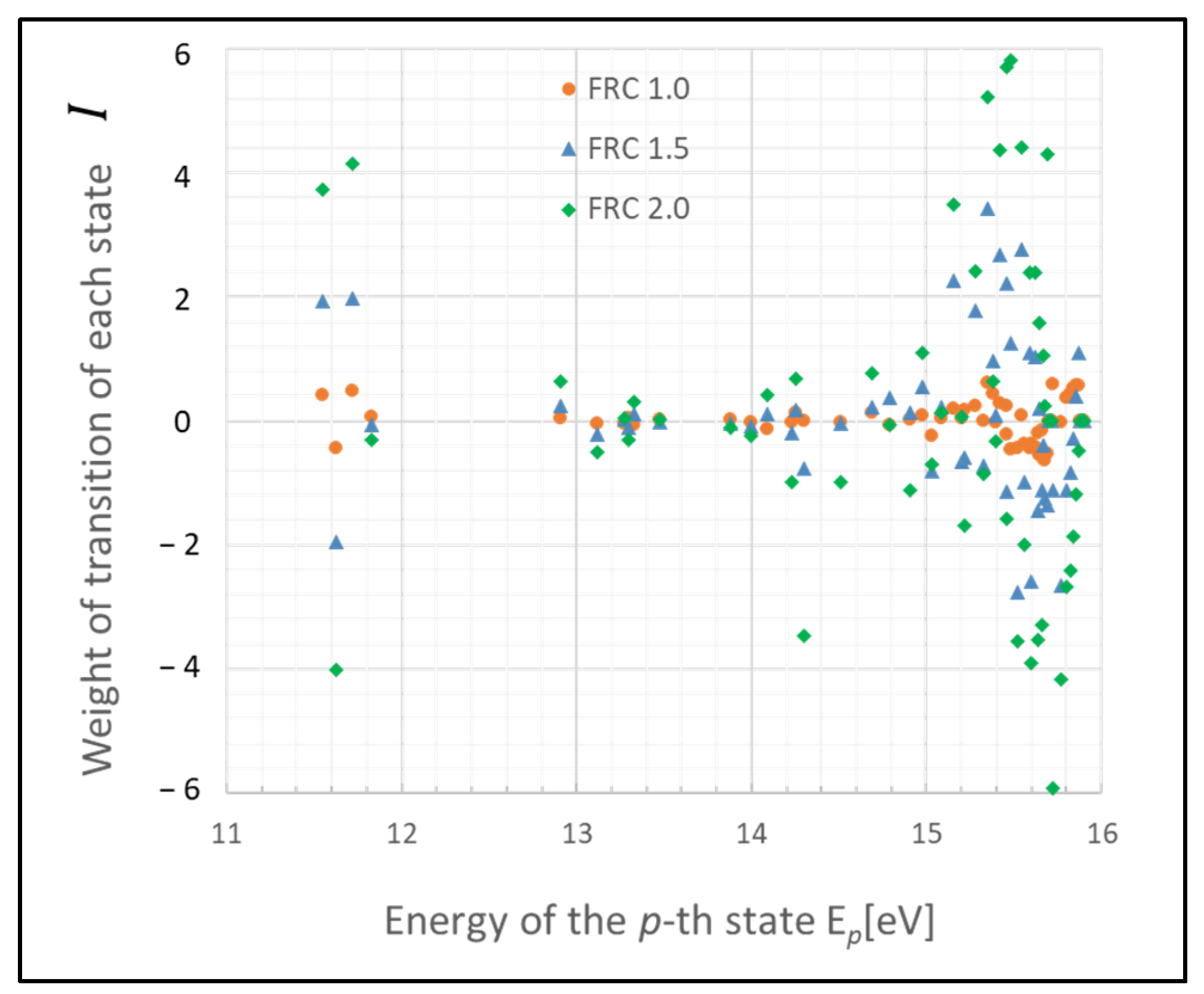
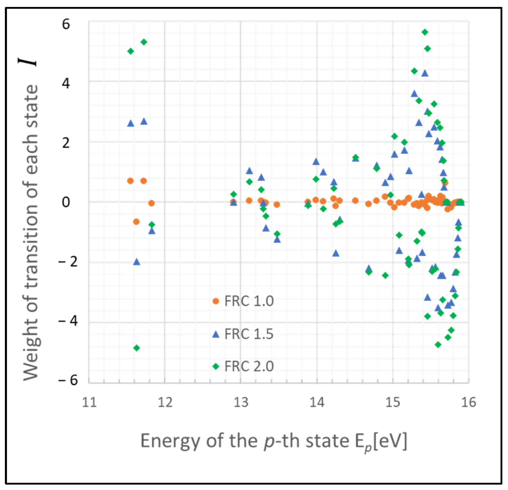
The graph in Figure 1 illustrates a scenario where the gas pressure is 1 Torr, the gas temperature Tg is 500 K, the electron temperature Te is 1 eV, and electron density Ne is 109 cm−3, with FRC indicating 2. The weight of each transition rate is defined as
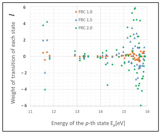
Figure 1.
Plots of non-adiabatic entropy weights in glow discharge plasma, calculated for each level using the revised model influenced by electron collisions. Dependency on the parameter FRC is illustrated (conditions: 1 Torr, 500 K, 1 eV, and 109 cm−3).
The weight of each transition exhibits varying levels of fluctuation in each state, with deviations from zero likely indicating the extent of influence of the Wiener process. Notably, atoms in states 2–4 (11.548–11.723 eV) and (14.509 eV) demonstrate substantial fluctuations based on FRC. This outcome is largely due to the infrequent radiative transitions, rendering these states predominantly influenced by collisional processes, which allow for atoms to survive longer. The discrepancy in the number density of excited-state atoms is particularly significant between states 2–4.
Furthermore, a substantial difference is noted in the tendency of fluctuations (i.e., increase or decrease) between the state and compared with that in Figure 2. This difference arises because the energy gaps in higher-energy states are smaller compared with those in lower-energy states.
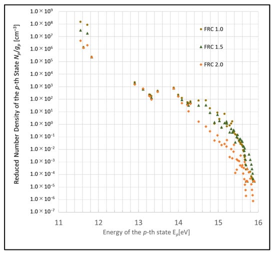
Figure 2.
Boltzmann plots illustrating the revised model due to electron collision and their dependency on the FRC parameter (conditions: 1 Torr, 500 K, 1 eV, and 109 cm−3).
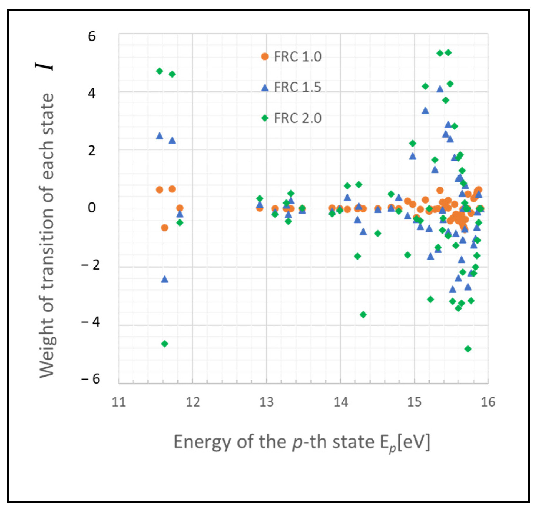
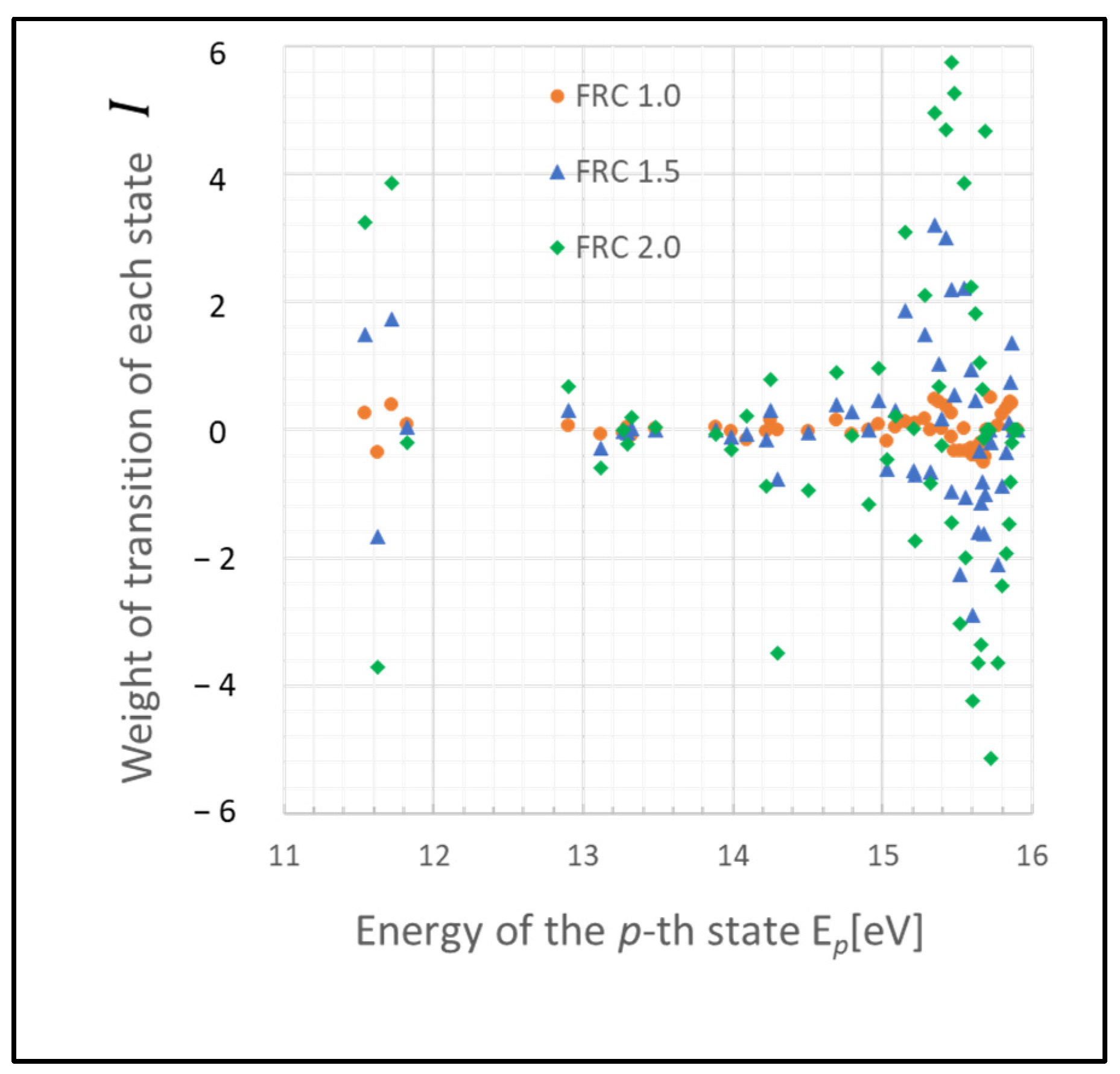
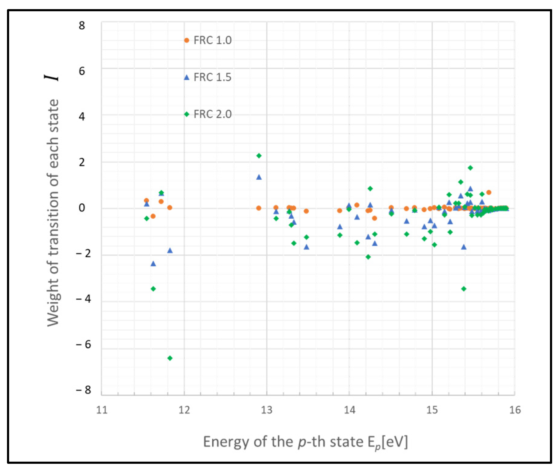
These states may function as a bottleneck in relaxing the entire plasma system to the steady state, as inferred from the relative entropy of the state. The graph in Figure 3 depicts the weight of the relative entropy for a case where the gas pressure is 0.1 Torr, with other parameters being the same as those shown in Figure 1. Comparing Figure 1 and Figure 3, an increase in the pressure of the discharge gas is observed to accelerate the convergence of non-adiabatic entropy. Similarly, Figure 4 represents another scenario where the gas temperature is 1000 K, with other parameters consistent with Figure 1. A comparison between the cases of Figure 1 and Figure 4 shows that an increase in the temperature of the discharge gas also slightly accelerates the convergence of non-adiabatic entropy.
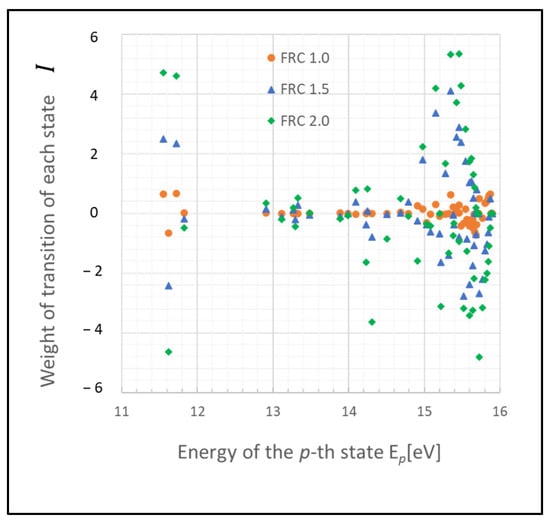
Figure 3.
Plots of non-adiabatic entropy weights in glow discharge plasma, calculated for each level using the revised model, influenced by electron collisions. Dependency on the parameter FRC is shown (conditions: 0.1 Torr, 500 K, 1 eV, and 109 cm−3).
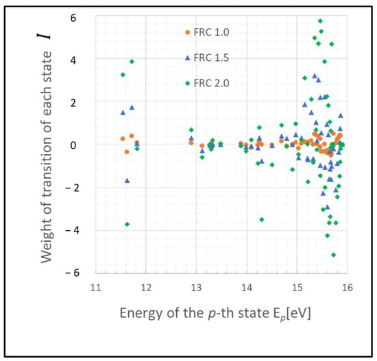
Figure 4.
Plots of non-adiabatic entropy weights in glow discharge plasma, calculated for each level using the revised model due to electron collisions. The dependency on the parameter FRC is depicted (conditions: 1 Torr, 1000 K, 1 eV, and 109 cm−3).
3.2. Arc Discharge
Arc discharge is extensively utilized in applications such as welding and arc lamps, and research into its utility in developing electric-propulsion spacecraft is ongoing. In a DC discharge tube, arc discharge occurs when the current is increased beyond that used for glow discharge. In contrast to nuclear fusion plasma, field emission has a weak contribution because its penetration gap is small and the density of volume electrons is high, and the discharge voltage is typically lower than that observed in glow discharge [33,34]. Compared to glow discharge, excitation and de-excitation due to electron collisions from adjacent levels are dominant, the slight contribution of far-away states makes the difference of each state small, and the system is close to the thermal equilibrium from Equation (19).
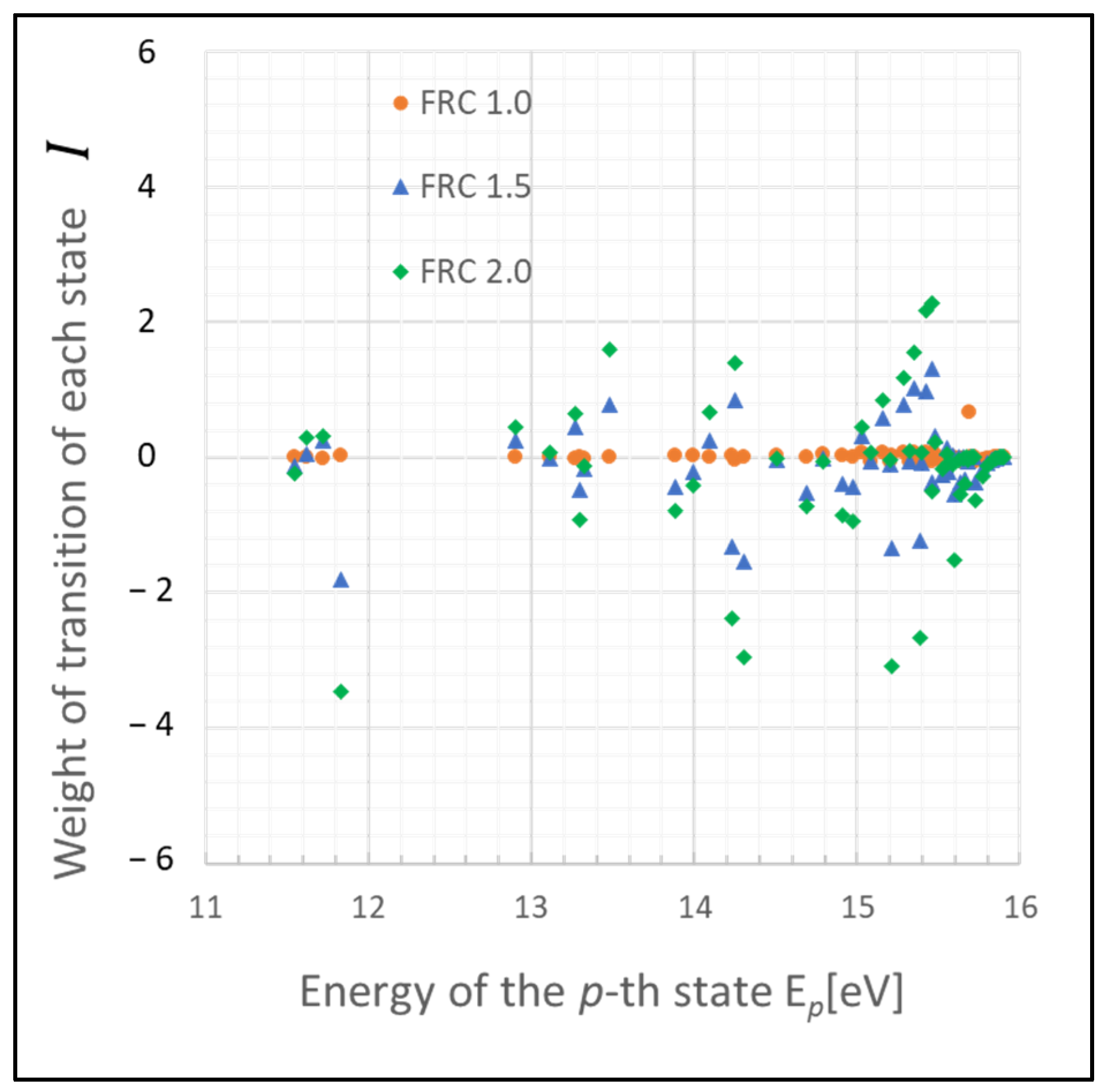
The graph in Figure 5 illustrates a scenario where the gas pressure is 760 Torr, the gas temperature is 500 K, the electron temperature is 2 eV, and the electron density is 1017 cm−3, with FRC indicating 2. The results from Figure 5 show that the convergence of states in arc discharge is faster than that observed in glow discharge, with the weights in the transition to a steady state being more uniformly distributed across all states. This indicates that the processes of electron collision and ground-state atomic collision occur at a relatively higher frequency in arc discharge compared with glow discharge, thereby reducing the time duration between transient and steady-state plasma.
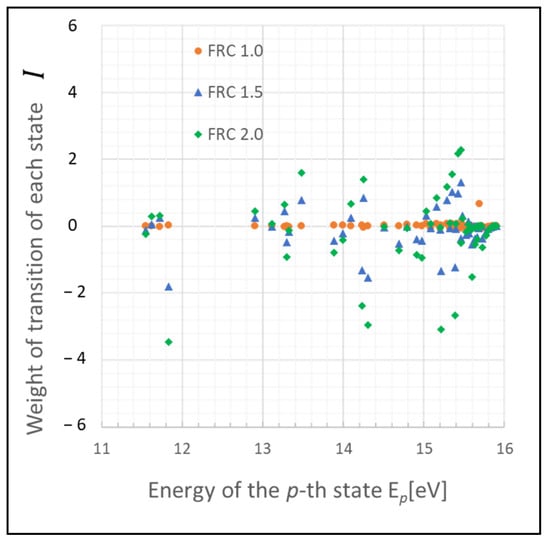
Figure 5.
Plots of non-adiabatic entropy weights in arc discharge plasma, calculated for each level using the revised model due to electron collisions. The dependency on the parameter FRC is demonstrated (conditions: 760 Torr, 500 K, 2 eV, and 1017 cm−3).
Particularly, in the case of CO2 laser weld of steel sheets, the influence of shielding gas types and flow rates have already studied [35]. For example, the tensile strength and formability of laser welds were studied, and they are strongly dependent upon the shielding gas types. Moreover, the shielding gas speed affects the weld width. In this plasma, it was reported that the fluctuation was caused and heat loss also produced. Our proposed method may be related to cases like this.
3.3. Recombining Plasma
In laboratory discharges, the cessation of the discharge process leads to the diffusion and recombination of charged species into neutral species, forming what is known as afterglow plasma [36]. This plasma also serves as a source of radicals generated from specialized discharges, which are transported to a chamber through a dedicated transport tube, a process referred to as “Remote Plasma” [37], where excited-state atoms are originated from the electron-ion recombination, rather than electron-impact excitation, since the electrons do not have sufficient energy for excitation.
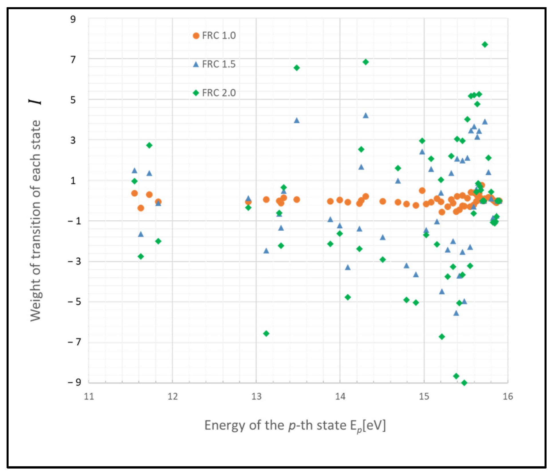
The graphs in Figure 6, Figure 7 and Figure 8 depict scenarios with a gas pressure of 0.0075 Torr and a temperature of 500 K, with FRC indicating 2. Figure 6 shows an electron density of 1013 cm−3 and an electron temperature of 0.2 eV. Figure 7 shows an electron density of 109 cm−3 and the same electron temperature of 0.2 eV. A comparison between the results of Figure 6 and Figure 7 reveals that as the electron density decreases, the states with high weights of relative entropy predominantly include lower-energy states (metastable states) and relatively high-energy states. Particularly, in high-energy states, an increase is noted in the high weight of relative entropy corresponding to the increase in energy due to energy flow dynamics.
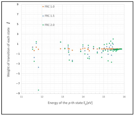
Figure 6.
Plots of non-adiabatic entropy weights in recombining plasma, calculated for each level using the revised model influenced by electron collisions. The dependency on the parameter FRC is illustrated (conditions: 0.0075 Torr, 500 K, 0.2 eV, and 1013 cm−3).
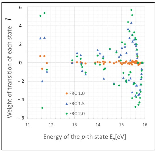
Figure 7.
Plots of non-adiabatic entropy weights in recombining plasma, calculated for each level using the revised model, influenced by electron collisions. Dependency on the parameter FRC is shown (conditions: 0.0075 Torr, 500 K, 0.2 eV, and 109 cm−3).

Figure 8.
Plots of non-adiabatic entropy weights in recombining plasma, calculated for each level using the revised model influenced by electron collisions. The plots illustrate the dependency on the parameter FRC (conditions: 0.0075 Torr, 500 K, 0.1 eV, and 1013 cm−3).
Figure 8 shows that although the electron density remains at 1013 cm−3, the electron temperature decreases to 0.1 eV, indicating a general decrease in the weight of relative entropy across almost all states compared with Figure 6. This indicates that lower electron temperatures lead to a decrease in the relative entropy across plasma states.
The graph in Figure 6 illustrates an increase in the dominance of relative entropy from around the middle of the states (about 14.5 eV) of the system, extending to both upper and lower states, suggesting two distinct energy flows originating from around the middle levels.
4. Discussion
Generally, when energy is transferred, fluctuation of entropy tends to be higher on the supply side compared with the demand side. Additionally, relative fluctuation of entropy is typically greater on the demand side than on the supply side [38].
denotes entropy generated in a low-temperature bath, denotes entropy generated in a high-temperature bath, and denotes time that is longer than a time step of the Wiener process. From Equation (21), the absolute value of the weight of each transition rate increases from the energy supply side to the energy demand side. The subscript of the entropy indicates cumulant and indicates moment. For example, .
However, in systems such as plasmas where radiative transitions serve as energy dissipation pathways, considering both the trend of relative fluctuation of entropy and the radiative process’s contribution to the lifetime is crucial [39]. In the report, statistical fluctuations in a steady-state system in a thermal equilibrium are influenced by external perturbations. They set response function as , an impulse changing the potential at time , in a quantity at time ,
From our results, the trend of relative fluctuation of entropy corresponds to the first term, and the lifetime of radiative processes corresponds to the second one.
For general thermodynamic systems described as Markov processes, a universal trade-off relation between efficiency and power is established [40]. The findings from plasma studies suggest that levels exhibiting high weights of relative entropy may be critical in facilitating the relaxation of the entire plasma system to a steady state. Controlling these levels selectively from the outside is essential for optimization, particularly from the perspective of energy efficiency.
In scenarios where the corona model does not apply, and cumulative excitation or de-excitation dominates in relatively high electron density environments, traditional methods such as the modified Boltzmann plot in the corona-phase region [41,42,43] may not be suitable [44]. Nevertheless, our evaluation method effectively reveals the direction and strength of these physical tendencies via calculation of the weight of each transition rate I defined in Equation (20).
In actual experimental situations involving glow discharge, fluctuations caused by ground-state atoms also occur, as demonstrated in Figure 9. Compared with fluctuations induced by electron collisions, a similar degree of weight across all levels is observed. This indicates that in the energy transport due to electron collisions, the weight on the transition to a steady state tends to be evened out across the system by collisions involving ground-state atoms. However, to simultaneously evaluate fluctuations due to electron collisions and fluctuations due to the ground-state atoms, it is thought that the contributions cannot be simply combined. Because when a measure in Wiener space shifts, only the direction in which the absolutely continuous measure shifts is considered, and the shift of the measure also changes the basis of another shift by .
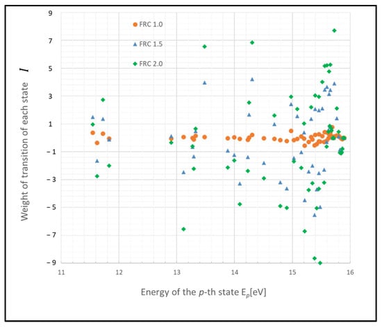
Figure 9.
Plots of non-adiabatic entropy weights in glow discharge plasma, calculated using the revised model for each level affected by collisions with ground-state atoms. The dependency on the parameter FRC is shown (conditions: 1 Torr, 500 K, 1 eV, and 109 cm−3).
denotes the connection of vector from one point to another one. Hence, using a tensor is necessary for the combination of two shifts. Particularly, depending on the order of each shift in the Wiener space, the difference of the combination of shifts is presumably to be evaluated by the product of the torsion tensor expressed in Equation (24) and the infinitesimal area spanned by these shifts [45,46].
In contrast, since the number of atoms at each level is always a positive value, a realistic method is to analyze the effects of electron collisions and ground-level atomic collisions alternately using the exponential gradient method with a non-negative matrix [47,48].
Overall, the results display a symmetrical tendency about the origin for each level and its adjacent levels. This symmetry suggests that when the stochastic flow locally between each level is considered, it is almost antisymmetric with respect to the exchange of states. Therefore, the positive and negative values in Equation (20) are relative. However, in complex physical models, the stationary distribution may be multi-modal due to nonlinear dependencies between parameters or latent (or hidden) variables [49].
For other plasmas, such as those naturally occurring or in fusion reactors, where plasma density and temperature differ from the studied cases, assessing the applicability of the CR model used in the above analysis is necessary. Despite limitations, this method could potentially be adapted for these plasmas by refining it from the perspective of entropy.
We did not evaluate plasma during the cooling process, where the EEDF shows strong departure from the Maxwell distribution. The self-consistent description of the EEDF and the population density remains as a future task.
5. Conclusions
An evaluation method is proposed to utilize relative entropy to predict plasma fluctuations based on a revised collisional–radiative model and fractional Brownian motion. Statistical analyses conducted via this method revealed that the transient behavior of plasma is characterized by both small and large fluctuations in each state. Information (i.e., I) is proposed as indicator to evaluate how far a system is from its steady state. These findings highlight the necessity of considering both the trend of entropy and the contribution of the radiative process to the lifetime. Additionally, states exhibiting high relative entropy weights may be critical in facilitating the relaxation of plasma to a steady state throughout the entire system.
Author Contributions
Conceptualization, Y.S.; Data curation, Y.S.; Formal analysis, Y.S.; Investigation, Y.S. and H.A.; Methodology, Y.S.; Project administration, H.A.; Resources, H.A.; Software, Y.S. and H.A.; Supervision, H.A.; Visualization, Y.S.; Writing—original draft, Y.S.; Writing—review and editing, H.A. All authors have read and agreed to the published version of the manuscript.
Funding
This research was funded partly by JSPS KAKENHI, grant number 22K03566.
Institutional Review Board Statement
“Not applicable” for studies not involving humans or animals.
Data Availability Statement
The original contributions presented in the study are included in the article, further inquiries can be directed to the corresponding author.
Conflicts of Interest
The authors declare no conflicts of interest.
Appendix A
The levels involved in the discharge argon plasma are summarized in Table A1 below.

Table A1.
Excited levels of Ar I considered in the present Ar CR model [18,50].
Table A1.
Excited levels of Ar I considered in the present Ar CR model [18,50].
| Level Number p | Designation | Excitation Energy (eV) | Statistical Weight | Level Number p | Designation | Excitation Energy (eV) | Statistical Weight |
|---|---|---|---|---|---|---|---|
| 1 | 3p6 | 0.000 | 1 | 35 | 6f, g, h | 15.382 | 216 |
| 2 | 4s[3/2]2 | 11.548 | 5 | 36 | 8p′ | 15.600 | 12 |
| 3 | 4s[3/2]1 | 11.624 | 3 | 37 | 8p | 15.423 | 24 |
| 4 | 4s′[1/2]0 | 11.723 | 1 | 38 | 7d′ + 9s′ | 15.636 | 24 |
| 5 | 4s′[1/2]1 | 11.828 | 3 | 39 | 7d + 9s | 15.460 | 48 |
| 6 | 4p[1/2]1 | 12.907 | 3 | 40 | 7f′, g′, h′, i′ | 15.659 | 160 |
| 7 | 4p[3/2]1,2, [5/2]2,3 | 13.116 | 20 | 41 | 7f, g, h, i | 15.481 | 320 |
| 8 | 4p′[3/2]1,2 | 13.295 | 8 | 42 | 8d′, f′, ⋯ | 15.725 | 240 |
| 9 | 4p′[1/2]1 | 13.328 | 3 | 43 | 8d, f, ⋯ | 15.548 | 480 |
| 10 | 4p[1/2]0 | 13.273 | 1 | 44 | 9p′, d′, f′, ⋯ | 15.769 | 320 |
| 11 | 4p′[1/2]0 | 13.480 | 1 | 45 | 9p, d, f, ⋯ | 15.592 | 640 |
| 12 | 3d[1/2]0,1, [3/2]2 | 13.884 | 9 | 46 | 10′ | 15.801 | 400 |
| 13 | 3d[7/2]3,4 | 13.994 | 16 | 47 | 10 | 15.624 | 800 |
| 14 | 3d′[3/2]2, [5/2]2,3 | 14.229 | 17 | 48 | 11′ | 15.825 | 484 |
| 15 | 5s′ | 14.252 | 4 | 49 | 11 | 15.648 | 968 |
| 16 | 3d[3/2]1, [5/2]2,3 + 5s | 14.090 | 23 | 50 | 12′ | 15.843 | 576 |
| 17 | 3d′[3/2]1 | 14.304 | 3 | 51 | 12 | 15.666 | 1152 |
| 18 | 5p | 14.509 | 24 | 52 | 13′ | 15.857 | 676 |
| 19 | 5p′ | 14.690 | 12 | 53 | 13 | 15.680 | 1352 |
| 20 | 4d + 6s | 14.792 | 48 | 54 | 14′ | 15.868 | 784 |
| 21 | 4d′ + gs′ | 14.976 | 24 | 55 | 14 | 15.691 | 1568 |
| 22 | 4f′ | 15.083 | 28 | 56 | 15′ | 15.877 | 900 |
| 23 | 4f | 14.906 | 56 | 57 | 15 | 15.700 | 1800 |
| 24 | 6p′ | 15.205 | 12 | 58 | 16′ | 15.884 | 1024 |
| 25 | 6p | 15.028 | 24 | 59 | 16 | 15.707 | 2048 |
| 26 | 5d′ + 7s′ | 15.324 | 24 | 60 | 17′ | 15.890 | 1156 |
| 27 | 5d + 7s | 15.153 | 48 | 61 | 17 | 15.713 | 2312 |
| 28 | 5f′, g′ | 15.393 | 64 | 62 | 18′ | 15.895 | 1296 |
| 29 | 5f, g | 15.215 | 128 | 63 | 18 | 15.718 | 2592 |
| 30 | 7p′ | 15.461 | 12 | 64 | 19′ | 15.899 | 1444 |
| 31 | 7p | 15.282 | 24 | 65 | 19 | 15.722 | 2888 |
| 32 | 6d′ + 8s′ | 15.520 | 24 | ||||
| 33 | 6d + 8s | 15.347 | 48 | ||||
| 34 | 6f′, g′, h′ | 15.560 | 108 |
Appendix B
In this study, the EEDF is assumed to be Maxwellian, following Fujimoto [19]. We admit that it will be necessary to solve the Boltzmann equation with the reduced electric field as the input in more detail. However, this is a future task and out of scope in the present study. First of all, this study considered the excited-state density distribution from an entropic standpoint, and in that sense, it is sufficient to discuss it under the assumption of a Maxwellian distribution. The excitation rate coefficient for Ar is provided as
In Equation (A1), represents the mass of the electron, and represents the threshold energy of the process. The double-subscript notation and in the electron collisional excitation cross-section denote the initial and final states of atoms, respectively (effective principal quantum number), following Vlček’s paper [18]. is the electron energy distribution function (EEDF), which is assumed to be Maxwellian in this study, which is formulated with normalization, , as below:
From Equation (A2), the average energy is Therefore, these numbers do not represent the principal quantum number. is determined based on the transition as described by an optically allowed transition
parity forbidden transitions
and spin forbidden transitions
In each equation, denotes the Bohr radius, denotes the ionization energy of hydrogen atoms, () denotes the normalized dimensionless energy, and are the fitting parameters, and denotes the oscillator strength for the case of an optically allowed transition.
Appendix C
Malliavin analysis evaluated the increase in Brownian motion. Brownian motion is expressed below. The increase in it is set as .
And the stochastic process is expressed below.
In this case, the Malliavin derivative is defined below. The maximum division of time set as .
Appendix D
The time variation of Kullback–Leibler information is expressed below.
References
- Conrads, H.; Schmidt, M. Plasma generation and plasma sources. Plasma Sources Sci. Technol. 2000, 9, 441–454. [Google Scholar] [CrossRef]
- Linke, J.; Du, J.; Loewenhoff, T.; Pintsuk, G.; Spilker, B.; Steudel, I.; Wirtz, M. Challenges for plasma-facing components in nuclear fusion. Matter Radiat. Extremes 2019, 4, 056201. [Google Scholar] [CrossRef]
- Freeman, J.; Harilal, S.; Diwakar, P.; Verhoff, B.; Hassanein, A. Comparison of optical emission from nanosecond and femtosecond laser produced plasma in atmosphere and vacuum conditions. Spectrochim. Acta Part B At. Spectrosc. 2013, 87, 43–50. [Google Scholar] [CrossRef]
- Kim, H.C.; Iza, F.; Yang, S.S.; Radmilović-Radjenović, M.; Lee, J.K. Particle and fluid simulations of low-temperature plasma discharges: Benchmarks and kinetic effects. J. Phys. D Appl. Phys. 2005, 38, R283–R301. [Google Scholar] [CrossRef]
- Capitelli, M.; Bruno, D.; Laricchiuta, A. Fundamental Aspects of Plasma Chemical Physics: Transport of Springer Series on Atomic, Optical, and Plasma Physics; Capitelli, M., Bruno, D., Laricchiuta, A., Eds.; Springer: New York, NY, USA, 2013. [Google Scholar]
- Colonna, G.; D’Angola, A. Plasma Modeling Methods and Applications; IOP Publishing: Bristol, UK, 2016; pp. 8–13. [Google Scholar]
- Jin, J.; Tu, M.W.-Y.; Zhang, W.-M.; Yan, Y. Non-equilibrium quantum theory for nanodevices based on the Feynman–Vernon influence functional. New J. Phys. 2010, 12, 083013. [Google Scholar] [CrossRef]
- Shiratani, M.; Koga, K. 2. Fluctuation of Low Pressure Processing Plasma and Growth of Nanoparticles. J. Plasma Fusion Res. 2014, 90, 378. [Google Scholar]
- Yamamoto, N.; Nakagawa, T.; Komurasaki, K.; Arakawa, Y. Discharge plasma fluctuations in hall thrusters. Vacuum 2001, 65, 375–381. [Google Scholar] [CrossRef]
- Kinoshita, M.; Fuyuto, T.; Akatsuka, H. Measurement of vibrational and rotational temperature in spark-discharge plasma by optical emission spectroscopy: Change in thermal equilibrium characteristics of plasma under air flow. Int. J. Engine Res. 2019, 20, 746–757. [Google Scholar] [CrossRef]
- Breden, D.; Raja, L.L.; Idicheria, C.A.; Najt, P.M.; Mahadevan, S. A numerical study of high-pressure non-equilibrium streamers for combustion ignition application. J. Appl. Phys. 2013, 114, 083302. [Google Scholar] [CrossRef]
- Okahara, A. Problems of Plasma Ignition System. DENSO TEN Tech. Rev. 2017, 1, 63–71. [Google Scholar]
- Starikovskiy, A. Physics and chemistry of plasma-assisted combustion. Philos. Trans. R. Soc. A Math. Phys. Eng. Sci. 2015, 373, 20150074. [Google Scholar] [CrossRef] [PubMed]
- Chung, B.; Rhee, S.; Lee, C. The effect of shielding gas types on CO2 laser tailored blank weldability of low carbon automotive galvanized steel. Mater. Sci. Eng. A 1999, 272, 357–362. [Google Scholar] [CrossRef]
- Komen, H.; Shigeta, M.; Tanaka, M. Numerical simulation of molten metal droplet transfer and weld pool convection during gas metal arc welding using incompressible smoothed particle hydrodynamics method. Int. J. Heat Mass Transf. 2018, 121, 978–985. [Google Scholar] [CrossRef]
- National Academies of Sciences. Engineering, and Medicine. In Plasma Science: Enabling Technology, Sustainability, Security, and Exploration; The National Academies Press: Washington, DC, USA, 2021. [Google Scholar] [CrossRef]
- Shimada, Y.; Akatsuka, H. Evaluating plasma fluctuation by collisional-radiative model using Malliavin derivative. Jpn. J. Appl. Phys. 2024, 63, 05SP02. [Google Scholar] [CrossRef]
- Vlček, J. A collisional-radiative model applicable to argon discharges over a wide range of conditions. I. Formulation and basic data. J. Phys. D 1989, 22, 623. [Google Scholar] [CrossRef]
- Fujimoto, T. Plasma Spectroscopy; Oxford University Press: Oxford, UK, 2004. [Google Scholar]
- Akatsuka, H. Discussion on Collisional Radiative Model from the Viewpoint of Linear Ordinary Differential Equations. In Proceedings of the 12th Asia Pacific Physics Conference (APPC12), Makuhari, Japan, 14–19 July 2013. [Google Scholar] [CrossRef]
- Malliavin, P. Stochastic calculus of variation and hypoelliptic operators. In Proceedings of the International Symposium on Stochastic Differential Equations, Kyoto, 1976; Wiley: New York, NY, USA; Wiley: Chichester, UK; Wiley: Brisbane, Australia, 1978; pp. 195–263. [Google Scholar]
- Kusuoka, S.; Stroock, D. Applications of the Malliavin calculus, Part i. In Stochastic Analysis; North-Holland Mathematical Library; Ito, K., Ed.; Elsevier: Amsterdam, The Netherlands, 1984; Volume 32, pp. 271–306. [Google Scholar]
- Kusuoka, S. Malliavin calculus revisited. J. Math. Sci. Univ. Tokyo 2003, 10, 261–278. [Google Scholar]
- Cameron, R.H.; Martin, W.T. Transformations of wiener integrals under translations. Ann. Math. 1944, 45, 386. [Google Scholar] [CrossRef]
- Mandelbrot, B.B.; Van Ness, J.W. Fractional Brownian Motions, Fractional Noises and Applications. SIAM Rev. 1968, 10, 422–437. [Google Scholar] [CrossRef]
- Hurst, H.E.; Black, R.P.; Simaika, Y.M. Long Term Storage in Reservoirs: An Experimental Study; Constable: London, UK, 1965. [Google Scholar]
- Falconer, K. Techniques in Fractal Geometry; John Wiley & Sons, Ltd.: Hoboken, NJ, USA, 1997. [Google Scholar]
- Hatano, T.; Sasa, S.-I. Steady-State Thermodynamics of Langevin Systems. Phys. Rev. Lett. 2001, 86, 3463–3466. [Google Scholar] [CrossRef] [PubMed]
- Kullback, S.; Leibler, R.A. On Information and Sufficiency. Ann. Math. Stat. 1951, 22, 79–86. [Google Scholar] [CrossRef]
- Goldston, R.J.; Rutherford, P.H. Introduction to Plasma Physics; Taylor & Francis Group: New York, NY, USA; Taylor & Francis Group: London, UK, 1995. [Google Scholar]
- Franz, G. Low Pressure Plasmas and Microstructuring Technology; Springer: Berlin, Germany, 2009. [Google Scholar] [CrossRef]
- Benilov, M.S. Multiple solutions in the theory of dc glow discharges and cathodic part of arc discharges. Application of these solutions to the modeling of cathode spots and patterns: A review. Plasma Sources Sci. Technol. 2014, 23, 054019. [Google Scholar] [CrossRef]
- Smirnov, B.M. Theory of Gas Discharge Plasma; Springer: Cham, Switzerland, 2015. [Google Scholar]
- Loureiro, J.; Amorim, J. Kinetics and Spectroscopy of Low Temperature Plasmas; Springer: Cham, Switzerland, 2016. [Google Scholar]
- Reisgen, U.; Schleser, M.; Mokrov, O.; Ahmed, E. Shielding gas influences on laser weldability of tailored blanks of advanced automotive steels. Appl. Surf. Sci. 2010, 257, 1401–1406. [Google Scholar] [CrossRef]
- Couëdel, L.; Mezeghrane, A.; Samarian, A.; Mikikian, M.; Tessier, Y.; Cavarroc, M.; Boufendi, L. Complex Plasma Afterglow. Contrib. Plasma Phys. 2009, 49, 235–259. [Google Scholar] [CrossRef]
- Fridman, A. Plasma Chemistry; Cambridge: New York, NY, USA, 2008; p. 531. [Google Scholar]
- Saryal, S.; Gerry, M.; Khait, I.; Segal, D.; Agarwalla, B.K. Universal Bounds on Fluctuations in Continuous Thermal Machines. Phys. Rev. Lett. 2021, 127, 190603. [Google Scholar] [CrossRef] [PubMed]
- Baiesi, M.; Maes, C.; Wynants, B. Fluctuations and Response of Nonequilibrium States. Phys. Rev. Lett. 2009, 103, 010602. [Google Scholar] [CrossRef]
- Shiraishi, N.; Saito, K.; Tasaki, H. Universal Trade-Off Relation between Power and Efficiency for Heat Engines. Phys. Rev. Lett. 2016, 117, 190601. [Google Scholar] [CrossRef]
- Gordillo-Vázquez, F.J.; Camero, M.; Gómez-Aleixandre, C. Spectroscopic measurements of the electron temperature in low pressure radiofrequency Ar/H2/C2H2 and Ar/H2/CH4 plasmas used for the synthesis of nanocarbon structures. Plasma Sources Sci. Technol. 2006, 15, 42. [Google Scholar] [CrossRef]
- Chung, T.H.; Kang, H.R.; Bae, M.K. Optical emission diagnostics with electric probe measurements of inductively coupled Ar/O2/Ar-O2 plasmas. Phys. Plasmas 2012, 19, 113502. [Google Scholar] [CrossRef]
- Tanişli, M.; Rafatov, I.; Şahin, N.; Mertadam, S.; Demir, S. Spectroscopic study and numerical simulation of low-pressure radio-frequency capacitive discharge with argon downstream. Can. J. Phys. 2017, 95, 190–200. [Google Scholar] [CrossRef]
- Akatsuka, H. Optical Emission Spectroscopic (OES) analysis for diagnostics of electron density and temperature in non-equilibrium argon plasma based on collisional-radiative model. Adv. Phys. X 2019, 4, 1592707. [Google Scholar] [CrossRef]
- Hehl, F.W.; Obukhov, Y.N. Éli Cartan’s torsion in geometry and in field theory, an essay. Ann. Fond. Louis Broglie 2007, 32, 157–194. [Google Scholar]
- Amari, S. Information Geometry and Its Applications; Springer: Cham, Switzerland, 2016; Volume 194. [Google Scholar]
- Cichocki, A.; Zdunek, R.; Amari, S.-I. Nonnegative Matrix and Tensor Factorization [Lecture Notes]. IEEE Signal Process. Mag. 2008, 25, 142–145. [Google Scholar] [CrossRef]
- Lee, D.D.; Seung, H.S. Learning the parts of objects by non-negative matrix factorization. Nature 1999, 401, 788–791. [Google Scholar] [CrossRef] [PubMed]
- Bishop, C.M.; Nasrabadi, N.M. Pattern Recognition and Machine Learning; Springer: New York, NY, USA, 2006; pp. 466–470. [Google Scholar]
- Mizuochi, J.; Sakamoto, T.; Matsuura, H.; Akatsuka, H. En Function in Microwave Discharge Plasmas by Spectroscopic Diagnostics with Collisional Radiative Model. Jpn. J. Appl. Phys. 2010, 49, 036001. [Google Scholar] [CrossRef]


Disclaimer/Publisher’s Note: The statements, opinions and data contained in all publications are solely those of the individual author(s) and contributor(s) and not of MDPI and/or the editor(s). MDPI and/or the editor(s) disclaim responsibility for any injury to people or property resulting from any ideas, methods, instructions or products referred to in the content. |
© 2024 by the authors. Licensee MDPI, Basel, Switzerland. This article is an open access article distributed under the terms and conditions of the Creative Commons Attribution (CC BY) license (https://creativecommons.org/licenses/by/4.0/).