Sampled-Data Exponential Synchronization of Complex Dynamical Networks with Saturating Actuators

Abstract

This paper investigates the problem of exponential synchronization control for complex dynamical systems (CDNs) with input saturation. Considering the effects of transmission delay, a memory sampled-data controller is designed. A modified two-sided looped functional is constructed that takes into account the entire sampling period, which includes both current state information and delayed state information. This functional only needs to be positive definite at the sampling instants. Sufficient criteria and the controller design method are provided to ensure the exponential synchronization of CDNs with input saturation under the influence of transmission delay, as well as the estimation of the basin of attraction. Additionally, an optimization algorithm for enlarging the region of attraction is proposed. Finally, a numerical example is presented to verify the effectiveness of the conclusion.

1. Introduction

In recent years, complex dynamical networks (CDNs) have garnered significant research attention due to their extensive applicability in various practical systems, such as biological networks, power grids, and communication networks [1,2,3]. The synchronization of these networks, a vital dynamic property, has become a focal point of study due to its relevance in fields like image recognition, secure communication, and information processing [4,5]. Numerous research findings on the synchronization problem of CDNs have been published [6,7,8,9,10,11]. The cluster synchronization for a class of CDNs with mismatched parameters was studied in [12]. Based on the free-weighting matrix approach and a fresh Lyapunov functional, the finite-time synchronization issue of CDNs was investigated in [13]. Considering the controller gains with uncertainties, the non-fragile synchronization control issues of CDNs were studied in [14,15,16].

As a crucial method in networked control, sampled-data control (SDC) only requires storing system information at sampling times, significantly reducing information transmission and thereby saving limited network bandwidth, making it more economical and feasible. Some significant results on sampled-data synchronization control for CDNs have been achieved [17,18,19,20,21,22]. The global $H_{\infty }$ pinning synchronization problem for CDNs via aperiodic SDC was explored in [18], using the input delay method and free-weighting matrix techniques. In [19], the condition for sampled-data synchronization of reaction–diffusion CDNs with semi-Markovian jumping topologies was presented. In [20], the synchronization problem of switched CDNs in a finite time sense was studied with an average dwell-time switching signal. For a class of fractional and impulsive complex networks with switching topologies at impulsive instants, a sampled-data-based event-triggered synchronization control was designed in [21]. By decomposing complex-valued dynamic systems into two real-valued systems, the synchronization of delayed complex-valued chaotic Lur’e systems was studied based on SDC in [22]. The sampling period is a key factor in SDC systems; a longer period can more effectively conserve network resources. Consequently, many researchers have been devoted to reducing conservatism in this aspect [23,24,25].

Actuator saturation frequently occurs in practical systems. Addressing input saturation is critical in controller design, as neglecting this issue can result in reduced system performance and potential instability [26]. Input saturation confines the system to achieve only local stability, with the precise determination of the basin of attraction (BoA) ensuring that stability is limited and challenging to ascertain accurately. Some scholars are dedicated to CDNs and have already carried out some meaningful work. Some synchronization criteria for continuous and discrete systems were presented in [27,28]. In [29], based on the aperiodic SDC method, the synchronization problem was studied and an optimal algorithm for the estimation of BoA was given. By designing parameter-dependent loop-based Lyapunov functionals, the design methods of sampled-data synchronization controller for polytopic uncertain switched CDNs were presented in [30]. Based on the aperiodic intermittent SDC method for complex-valued stochastic systems, the mean-squared exponential synchronization problem was studied in [31]. However, the effect of transmission delay is not considered in these results. Due to the delay in sending the updated signal from the sampler to the controller and then to the zero-order holder, it is necessary to design a memory sampling controller that accounts for transmission delay. Although some significant results for CDNs have considered transmission delay $\mu$, only the information at time $t_{\kappa }$ has been taken into account. Furthermore, considering the input saturation, the question of how to design a memory sampling controller that incorporates comprehensive information about the accessible characteristics of the real sampling pattern and provides an estimation of the BoA is a significant problem to be solved.

According to the above analysis, the main purpose of this paper is to solve the exponential synchronization issue of CDNs and provide the design method of a memory sampled-data controller. The following is a brief description of the main work and innovation:

(1)

Considering the influence of input saturation and transmission delay, an exponential sampled-data synchronization control scheme for CDNs is proposed.

(2)

A new two-sided looped-functional containing complete sampling interval information is constructed, and the delay states $z(t_{\kappa }-\mu )$ and $z(t_{\kappa +1}-\mu )$ are also taken into account.

(3)

Based on the memory SDC strategy and the constructed functional, the estimation of BoA and the corresponding optimization algorithm are given.

The remainder of this paper is organized as follows. In Section 2, the model description and some necessary preliminary knowledge are briefly outlined. The main theoretical conclusion is given in Section 3. In Section 4, a numerical simulation is chosen to validate the effectiveness of the proposed method. Section 5 is the conclusion.

Notation 1.

${\mathbb{S}}_j=\{1,2,\dots ,j\}$. $\mathrm{diag}\{\cdots \}$ and $\mathrm{col}\{\cdots \}$ represent the block diagonal matrix and column vector or matrix, respectively. $\mathrm{Sym}\left\{V\right\}=V+V^T$.

2. Model Description and Preliminaries

Consider the following CDNs with actuator saturation:

$$\begin{array}{cc}& {\dot{x}}_i\left(t\right)=-f\left(x_i\left(t\right)\right)+c{\displaystyle \sum _{j=1}^N}{a}_{ij}B{x}_i\left(t\right)+\mathrm{sat}\left(u_i\left(t\right)\right)\hfill \end{array}$$

(1)

for $i\in {\mathbb{S}}_N$, where N is the number of coupled nodes; $x_i\left(t\right)\in {\mathbb{R}}^n$ denotes the state vector; c is the coupling strength; $A={\left[a_{ij}\right]}_{N\times N}$ and $B\in {\mathbb{R}}^{n\times n}$ are the external and internal coupling matrices, respectively; Matrix A satisfies the zero-row-sum condition, where $a_{ij}>0$ if nodes i and j are connected, and $a_{ij}=0$ otherwise. $f\left(x_i\left(t\right)\right):{\mathbb{R}}^n\to {\mathbb{R}}^n$ is a nonlinear function; $u_i\left(t\right)$ represents the control input; the saturation function $\mathrm{sat}\left(u_i\left(t\right)\right)={[\mathrm{sat}\left(u_{i1}\left(t\right)\right),\mathrm{sat}\left(u_{i2}\left(t\right)\right),\dots ,\mathrm{sat}\left(u_{in}\left(t\right)\right)]}^T$ is defined as:

$$\begin{array}{c}\hfill \mathrm{sat}\left(u_{il}\left(t\right)\right)=\mathrm{sgn}\left(u_{il}\left(t\right)\right)min\{u_{0l},|u_l\left(t\right)\left|\right\},l\in {\mathbb{S}}_n\end{array}$$

where $u_{0l}>0$ represents the saturation threshold.

Consider the isolated node as follows:

$$\begin{array}{c}\hfill \dot{y}\left(t\right)=f\left(y\left(t\right)\right),y\left(t\right)\in {\mathbb{R}}^n.\end{array}$$

(2)

Denote the error vectors $z_i\left(t\right)=x_i\left(t\right)-y\left(t\right)$, and $f\left(z_i\left(t\right)\right)=f\left(x_i\left(t\right)\right)-f\left(y\left(t\right)\right)$, the error system can be expressed as

$$\begin{array}{cc}\hfill {\dot{z}}_i\left(t\right)=& -f\left(z_i\left(t\right)\right)+c{\displaystyle \sum _{j=1}^N}{a}_{ij}B{z}_i\left(t\right)+\mathrm{sat}\left(u_i\left(t\right)\right)\hfill \end{array}$$

(3)

The control signal is transmitted to the plant via the zero-order Hold, utilizing the following hold-time sequence: $0=t_0<t_1\cdots <{\displaystyle \underset{\kappa \to \infty }{lim}}{t}_{\kappa }=+\infty$. The sampling interval $t_{\kappa +1}-t_{\kappa }=h_{\kappa }\in (\check{h},\widehat{h}]$, $\forall \kappa \ge 0$, is the aperiodic sampling interval, which falls within the range $(\check{h},\widehat{h}]$.

Consider the SDC input $u_i\left(t\right)$ with transmission delay $\mu$ as follows:

$$\begin{array}{cc}& u_i\left(t\right)=K_{1i}{z}_i\left(t_{\kappa }\right)+K_{2i}{z}_i(t_{\kappa }-\mu ),t\in [t_{\kappa },t_{\kappa +1})\hfill \end{array}$$

(4)

where $K_{1i}$ and $K_{2i}$ are the controller gain matrices to be designed with appropriate dimensions.

Define the following dead-zone nonlinear function:

$$\begin{array}{cc}& \Psi \left(u_i\left(t\right)\right)\triangleq {\Psi }_{\kappa }^i=u_i\left(t\right)-\mathrm{sat}\left(u_i\left(t\right)\right).\hfill \end{array}$$

(5)

Substituting (5) into (1), the closed-loop system can be given as

$$\begin{array}{cc}\hfill \dot{z}\left(t\right)=& F\left(z\left(t\right)\right)+c(A\otimes B)z\left(t\right)+\mathcal{K}{\eta }_1\left(t_{\kappa }\right)-{\Psi }_{\kappa }\hfill \end{array}$$

(6)

where $z\left(t\right)={[z_1^T\left(t\right),z_2^T\left(t\right),\dots ,z_N^T\left(t\right)]}^T$, $\mathcal{K}=[K_1,K_2]$, $K_1=\mathrm{diag}\{K_{11},K_{12},\dots ,K_{1N}\}$, $K_2=\mathrm{diag}\{K_{21},K_{22},\dots ,K_{2N}\}$, ${\eta }_1\left(t_{\kappa }\right)={[z^T\left(t_{\kappa }\right),z^T(t_{\kappa }-\mu )]}^T$, ${\Psi }_{\kappa }={[{\Psi }_{\kappa }^{1T},{\Psi }_{\kappa }^{2T},\dots ,{\Psi }_{\kappa }^{NT}]}^T$, $F\left(z\left(t\right)\right)={[F^T\left(z_1\left(t\right)\right),F^T\left(z_2\left(t\right)\right),\dots ,F^T\left(z_N\left(t\right)\right)]}^T$.

The following hypotheses and lemmas are given to facilitate the subsequent theoretical analysis.

Assumption 1.

For any $r,s\in {\mathbb{R}}^n$, $f_{rs}=f\left(r\right)-f\left(s\right)$, constant matrices $L_1$ and $L_2$, $f_{rs}$ satisfies

$$\begin{array}{c}\hfill {[f_{rs}-L_1(r-s)]}^T[f_{rs}-L_2(r-s)]\le 0.\end{array}$$

(7)

Lemma 1

([32]). Let $s(·):[p,q]\to {\mathbb{R}}^n$ be a differentiable function, and $\mathcal{V}>0$ be any matrix. Then the following inequality holds:

$$\begin{array}{c}\hfill (p-q){\int }_q^p{\dot{s}}^T\left(s\right)\mathcal{V}\dot{s}\left(s\right)ds\ge {\mathfrak{S}}_1^T\mathcal{V}{\mathfrak{S}}_1+3{\mathfrak{S}}_2^T\mathcal{V}{\mathfrak{S}}_2\end{array}$$

where ${\mathfrak{S}}_1=s\left(p\right)-s\left(q\right)$, ${\mathfrak{S}}_2=s\left(p\right)+s\left(q\right)-\frac{2}{p-q}{\int }_q^{p}s\left(s\right)ds$.

Lemma 2

([33]). For a scalar $0<b<1$, $\mathfrak{U},{\mathfrak{U}}^{\prime }\in {\mathbb{R}}^n$, positive definite matrices ${ћ}_1,{ћ}_2\in {\mathbb{R}}^{n\times n}$, and any matrices $\mathfrak{Y},{\mathfrak{Y}}^{\prime }\in {\mathbb{R}}^{n\times n}$, the following inequality is satisfied:

$$\begin{array}{cc}& \frac{1}{\pi }{\mathfrak{U}}^T{ћ}_1\mathfrak{U}+\frac{1}{1-\pi }{\mathfrak{U}}^{\prime T}{ћ}_2{\mathfrak{U}}^{\prime }\hfill \\ & \ge {\mathfrak{U}}^T[{ћ}_1+(1-\pi )({ћ}_1-\mathfrak{Y}{ћ}_2^{-1}{\mathfrak{Y}}^T)]\mathfrak{U}+2{\mathfrak{U}}^T[\pi \mathfrak{Y}\hfill \\ & +(1-\pi ){\mathfrak{Y}}^{\prime }]{\aleph }_2+{\mathfrak{U}}^{\prime T}[{ћ}_2+\pi ({ћ}_2-{\mathfrak{Y}}^{\prime T}{ћ}_1^{-1}{\mathfrak{Y}}^{\prime T})]{\mathfrak{U}}^{\prime }.\hfill \end{array}$$

Lemma 3

([23]). For a positive definite matrix A and a nonsingular matrix B, let $A^{\prime }=B^{T}AB$, if the matrix inequality

$$\begin{array}{c}\hfill \left[\begin{array}{cc}\wp & I\\ I& B+B^T-A^{\prime }\end{array}\right]>0\end{array}$$

holds, then $A<\wp$.

3. Main Result

In this section, the design method for the sampling controller will be presented, and the criteria to ensure local stability of the error system (6) will be proposed. For convenience, the following symbols are defined:

$$\begin{array}{cc}& \mathcal{H}=t-t_{\kappa },{\mathcal{H}}^{\prime }=t_{\kappa +1}-t,r_0=0_{Nn\times 13Nn},\hfill \\ & r_{†}=\left[\begin{array}{ccc}{0}_{Nn\times (†-1)Nn}& I_{Nn}& 0_{Nn\times (13-†)Nn}\end{array}\right],†\in {\mathbb{S}}_{13}\hfill \\ & {\eta }_1\left(t\right)=\mathrm{col}\{z\left(t\right),z(t-\mu )\},{\eta }_2\left(t\right)=col\{z\left(t\right),\dot{z}\left(t\right)\}\hfill \\ & {\chi }_1\left(t\right)=\mathrm{col}\{z\left(t\right)-z\left(t_{\kappa }\right),z(t-\mu )-z(t_k-\mu )\}\hfill \\ & {\chi }_2\left(t\right)=\mathrm{col}\{z\left(t_{\kappa +1}\right)-z\left(t\right),z(t_{k+1}-\mu )-z(t-\mu )\}\hfill \\ & {\chi }_3\left(t\right)=\mathrm{col}\{{\mathcal{H}}^{\prime }{\chi }_1\left(t\right),\mathcal{H}{\chi }_2\left(t\right)\},{\chi }_4\left(t\right)=\mathrm{col}\{{\chi }_1\left(t\right),{\chi }_2\left(t\right))\}\hfill \\ & {\chi }_5\left(t\right)=\mathrm{col}\{z\left(t_{\kappa }\right),z\left(t_{\kappa +1}\right),z(t_{\kappa }-\mu ),z(t_{\kappa +1}-\mu )\},\hfill \\ & {\chi }_6\left(t\right)=\mathrm{col}\{{\chi }_5\left(t\right),v_1\left(t\right),v_2\left(t\right)\}\hfill \\ & \mathcal{N}\left(t\right)=\mathrm{col}\{{\eta }_2\left(t\right),{\eta }_2(t-\mu ),{\chi }_5\left(t\right),v_1\left(t\right),v_2\left(t\right),v_3\left(t\right),F\left(z\left(t\right)\right),{\Psi }_k\}\hfill \\ & v_1\left(t\right)=\frac{1}{\mathcal{H}}{\int }_{t_{\kappa }}^{t}z\left(s\right)ds,v_2\left(t\right)=\frac{1}{{\mathcal{H}}^{\prime }}{\int }_t^{t_{\kappa +1}}z\left(s\right)ds,v_3\left(t\right)=\frac{1}{\mu }{\int }_{t-\mu }^{t}z\left(s\right)ds,\hfill \\ & {\mathbb{L}}_1=0.5{(I\otimes L_1)}^T(I\otimes L_2)+0.5{(I\otimes L_2)}^T(I\otimes L_1),\hfill \\ & {\mathbb{L}}_2=-0.5{(I\otimes L_1)}^T-0.5{(I\otimes L_2)}^T,\mathbb{L}=\left[\begin{array}{cc}{\mathbb{L}}_1& {\mathbb{L}}_2\\ ★& I\end{array}\right].\hfill \end{array}$$

Theorem 1.

For given scalars ${ϵ}_1>0$, $h>0$, if there exist positive matrices $P\in {\mathbb{R}}^{2nN\times 2nN}$, $O_{\rho }\in {\mathbb{R}}^{nN\times nN}$, $R_1\in {\mathbb{R}}^{2nN\times 2nN}$, and $R_2\in {\mathbb{R}}^{nN\times nN}$, symmetric matrix $Y\in {\mathbb{R}}^{6nN\times 6nN}$, arbitrary matrices $S_{\rho }\in {\mathbb{R}}^{4nN\times 4nN}$, $X\in {\mathbb{R}}^{2nN\times 2nN}$, $Y_1\in {\mathbb{R}}^{2nN\times 2nN}$, $Y_2\in {\mathbb{R}}^{2nN\times 2nN}$, $G_{\psi }\in {\mathbb{R}}^{nN\times nN}$, $K_j\in {\mathbb{R}}^{nN\times nN}$ and $J\in {\mathbb{R}}^{nN\times 2nN}$, $\psi \in {\mathbb{S}}_2$, and diagonal positive matrix ${\Lambda }_1\in R^{nN\times nN}$ such that

$$\begin{array}{cc}& {\Omega }^1=\left[\begin{array}{cc}{E}^1+h_k{E}^2& {\Pi }_1^T{Y}_1\\ ★& -O_2^{\prime }\end{array}\right]<0\hfill \end{array}$$

(8)

$$\begin{array}{cc}& {\Omega }^2=\left[\begin{array}{cc}{E}^1+h_k{E}^3& {\Pi }_2^T{Y}_2^T\\ ★& -O_1^{\prime }\end{array}\right]<0\hfill \end{array}$$

(9)

$$\begin{array}{c}\hfill \left[\begin{array}{cc}P& {({\mathcal{K}}_{\left(j\right)}-J_{\left(j\right)})}^T\\ ★& U_{0j}^2\end{array}\right]>0\end{array}$$

(10)

where

$$\begin{array}{cc}\hfill E^1=& \mathrm{sym}\left\{{{\Phi }_1^1}^{T}P{\Phi }_1^2+{\Omega }_3^{5T}(S_1{\Omega }_4^1+S_2{\Omega }_5)+{\Omega }_1^{2T}X{\Omega }_2^1+{\Omega }_1^{1T}X{\Omega }_2^2\right\}-{\Pi }_1^T{O}_1^{\prime }{\Pi }_1\hfill \\ & -{\Pi }_2^T{O}_2^{\prime }{\Pi }_2+{{\Phi }_2^1}^T{R}_1{\Phi }_2^1-{{\Phi }_2^2}^T{R}_1{\Phi }_2^2+\mathrm{sym}\left\{r_{13}^T{\Lambda }_{1}J{\Phi }_1^3-r_{13}^T{\Lambda }_1{r}_{13}\right\}\hfill \\ & +{\mu }^2{r}_2^T{R}_2{r}_2-{{\Phi }_0^1}^T{R}_2{\Phi }_0^1-3{{\Phi }_0^2}^T{R}_2{\Phi }_0^2-{ϵ}_1{\mathfrak{E}}^T\mathbb{L}\mathfrak{E}+\Gamma \hfill \\ \hfill E^2=& \mathrm{sym}\left\{{\Omega }_3^{1T}{S}_1{\Omega }_4^2+{\Omega }_3^{3T}(S_1{\Omega }_4^1+S_2{\Omega }_5)+{\Omega }_6^{2T}Y{\Omega }_6^1-\frac{1}{h_{\kappa }}{\Pi }_1^T{Y}_2{\Pi }_2\right\}\hfill \\ & +{\Omega }_6^{1T}Y{\Omega }_6^1+h_{\kappa }{r}_2^T{O}_1{r}_2-\frac{1}{h_{\kappa }}{\Pi }_1^T{O}_1^{\prime }{\Pi }_1\hfill \\ \hfill E^3=& \mathrm{sym}\left\{{\Omega }_3^{2T}{S}_1{\Omega }_4^2+{\Omega }_3^{4T}(S_1{\Omega }_4^1+S_2{\Omega }_5)+{\Omega }_6^{3T}Y{\Omega }_6^1-\frac{1}{h_{\kappa }}{\Pi }_1^T{Y}_1{\Pi }_2\right\}\hfill \\ & -{\Omega }_6^{1T}Y{\Omega }_6^1+h_{\kappa }{r}_2^T{O}_2{r}_2-\frac{1}{h_{\kappa }}{\Pi }_2^T{O}_2^{\prime }{\Pi }_2\hfill \\ \hfill {\Gamma }_0=& {\rho }_1{r}_1^T{G}^T+{\rho }_2{r}_2^T{G}^T,\mathfrak{E}=col\{r_1,r_{12}\}\hfill \\ \hfill \Gamma =& \mathrm{sym}\left\{{\Gamma }_0(-r_2+r_{12}+C(A\otimes B)r_1+\mathcal{K}{\Phi }_1^3-r_{13})\right\}\hfill \\ \hfill {\Pi }_1=& col\{r_1-r_5,r_1+r_5-2r_9\},{\Omega }_1^1=\{r_1-r_5,r_3-r_7\},{\Omega }_1^2=\{r_2,r_4\}\hfill \\ \hfill {\Pi }_2=& col\{r_6-r_1,r_1+r_6-2r_{10}\},{\Omega }_2^1=\{r_6-r_1,r_8-r_3\},{\Omega }_2^2=-{\Omega }_1^2\hfill \\ \hfill {\Omega }_3^1=& col\{{\Omega }_1^1,r_0,r_0\},{\Omega }_3^2=col\{r_0,r_0,{\Omega }_2^1\},{\Omega }_3^3=col\{{\Omega }_1^2,r_0,r_0\},{\Omega }_3^4=col\{r_0,r_0,{\Omega }_2^2\}\hfill \\ \hfill {\Omega }_3^5=& col\{-{\Omega }_1^1,{\Omega }_2^1\},{\Omega }_4^1=col\{{\Omega }_1^1,{\Omega }_2^1\},{\Omega }_4^2=col\{{\Omega }_1^2,{\Omega }_2^2\}{\Omega }_5=col\{r_5,r_6,r_7,r_8\},\hfill \\ \hfill {\Omega }_6^1=& col\{{\Omega }_5,r_9,r_{10}\},{\Phi }_0^1=r_1-r_3,{\Omega }_6^2=col\{r_0,r_0,r_0,r_0,r_1-r_9,r_0\},\hfill \\ \hfill {\Omega }_6^3=& col\{r_0,r_0,r_0,r_0,r_0,r_{10}-r_1\},{\Phi }_0^2=r_1+r_3-2r_{11},{\Phi }_1^1=\{r_1,r_3\}\hfill \\ \hfill {\Phi }_2^1=& \{r_1,r_2\},{\Phi }_2^2=\{r_3,r_4\},{\Phi }_1^3=\{r_5,r_7\},{\Phi }_1^2=\{r_2,r_4\}\hfill \end{array}$$

then the error system (6) is stable for any initial condition $z\left(t_0\right)\in \mathfrak{E}\left(P\right)=\left\{z\left(t_0\right)\in {\mathbb{R}}^{nN}\mid {♮}_2\underset{-r\le s\le 0}{sup}\{\parallel z\left(s\right){\parallel }^2,\parallel \dot{z}\left(s\right){\parallel }^2\}\le 1\right\}$.

Proof. 

Consider the following two-sided looped-functional:

$$\begin{array}{c}\hfill V\left(t\right)=V_1\left(t\right)+V_2\left(t\right)+V_3\left(t\right)+V_4\left(t\right)\end{array}$$

(11)

where

$$\begin{array}{cc}\hfill V_1\left(t\right)& ={\eta }_1^T\left(t\right)P{\eta }_1\left(t\right)\hfill \\ \hfill V_2\left(t\right)& =2{\chi }_3^T\left(t\right)\left(S_1{\chi }_4\left(t\right)+S_2{\chi }_5\left(t\right)\right)+2{\chi }_1^T\left(t\right)X{\chi }_2\left(t\right)\hfill \\ \hfill V_3\left(t\right)& =\mathcal{H}{\mathcal{H}}^{\prime }{\chi }_6^T\left(t\right)Y{\chi }_6\left(t\right)\hfill \\ \hfill V_4\left(t\right)& ={\mathcal{H}}^{\prime }{h}_{\kappa }{\int }_{t_{\kappa }}^t{\dot{z}}^T\left(s\right)O_1\dot{z}\left(s\right)ds-\mathcal{H}{h}_{\kappa }{\int }_t^{t_{\kappa +1}}{\dot{z}}^T\left(s\right)O_2\dot{z}\left(s\right)ds\hfill \\ \hfill V_5\left(t\right)& ={\int }_{t-\mu }^t{\eta }_2^T\left(s\right)R_1{\eta }_2\left(s\right)ds+\mu {\int }_{-\mu }^0{\int }_{t+\phi }^t{\dot{z}}^T\left(s\right)R_2\dot{z}\left(s\right)dsd\phi .\hfill \end{array}$$

Calculating the time derivative of $V\left(t\right)$ yields

$$\begin{array}{cc}\hfill {\dot{V}}_1\left(t\right)=& {\dot{\eta }}_1{\left(t\right)}^{T}P{\eta }_1\left(t\right)+{\eta }_1^T\left(t\right)P{\dot{\eta }}_1\left(t\right)\hfill \end{array}$$

(12)

$$\begin{array}{cc}\hfill {\dot{V}}_2\left(t\right)=& 2{\dot{\chi }}_1^T\left(t\right)X{\chi }_2\left(t\right)+2{\chi }_1^T\left(t\right)X{\dot{\chi }}_2\left(t\right)+2{\dot{\chi }}_3^T\left(t\right)(S_1{\chi }_4\left(t\right)+S_2{\chi }_5\left(t\right))\hfill \\ & +2{\dot{\chi }}_1^T\left(t\right)X{\chi }_2\left(t\right)+2{\chi }_1^T\left(t\right)X{\dot{\chi }}_2\left(t\right)\hfill \end{array}$$

(13)

$$\begin{array}{cc}\hfill {\dot{V}}_3\left(t\right)=& 2\mathcal{H}{\mathcal{H}}^{\prime }{\dot{\chi }}_6^T\left(t\right)Y{\chi }_6\left(t\right)+{\mathcal{H}}^{\prime }{\chi }_6^T\left(t\right)Y{\chi }_6\left(t\right)-\mathcal{H}{\chi }_6^T\left(t\right)Y{\chi }_6\left(t\right)\hfill \end{array}$$

(14)

$$\begin{array}{cc}\hfill {\dot{V}}_4\left(t\right)=& {\mathcal{H}}^{\prime }{h}_{\kappa }{\dot{z}}^T\left(t\right)O_1\dot{z}\left(t\right)+\mathcal{H}{h}_{\kappa }{\dot{z}}^T\left(t\right)O_2\dot{z}\left(t\right)\hfill \\ & -h_{\kappa }{\int }_{t_{\kappa }}^t{\dot{z}}^T\left(s\right)O_1\dot{z}\left(s\right)ds-h_{\kappa }{\int }_t^{t_{\kappa +1}}{\dot{z}}^T\left(s\right)O_2\dot{z}\left(s\right)ds\hfill \end{array}$$

(15)

$$\begin{array}{cc}\hfill {\dot{V}}_5\left(t\right)=& {\eta }_2^T\left(t\right)R_1{\eta }_2\left(t\right)-{\eta }_2^T(t-\mu )R_1{\eta }_2(t-\mu )\hfill \\ & +{\mu }^2{\dot{z}}^T\left(t\right)R_2\dot{z}\left(t\right)-\mu {\int }_{t-\mu }^t{\dot{z}}^T\left(s\right)R_2\dot{z}\left(s\right)ds\hfill \end{array}$$

(16)

By applying Lemma 1, we have

$$\begin{array}{cc}& \mu {\int }_{t-\mu }^t{\dot{z}}^T\left(s\right)R_2\dot{z}\left(s\right)ds\hfill \\ & \ge {\mathcal{N}}^T\left(t\right)\left[{\Phi }_0^{1T}{R}_2{\Phi }_0^1+3{\Phi }_0^{2T}{R}_2{\Phi }_0^2)\right]\mathcal{N}\left(t\right).\hfill \end{array}$$

(17)

From Lemmas 1 and 2, it can be inferred that

$$\begin{array}{cc}& -h_{\kappa }{\int }_{t_{\kappa }}^t{e}^{2as}{\dot{z}}^T\left(s\right)O_1\dot{z}\left(s\right)ds-h_{\kappa }{\int }_t^{t_{\kappa +1}}{\dot{z}}^T\left(s\right)O_2\dot{z}\left(s\right)ds\hfill \\ & \le -\left[\frac{h_{\kappa }}{\mathcal{H}}{\mathcal{Q}}_1^T{\mathfrak{O}}_1{\mathcal{Q}}_1+\frac{h_{\kappa }}{{\mathcal{H}}^{\prime }}{\mathcal{Q}}_2^T{\mathfrak{O}}_2{\mathcal{Q}}_2\right]\hfill \\ & \le -{\mathcal{N}}^T\left(t\right)[{\Pi }_1^T\left({\mathfrak{O}}_1+\frac{{\mathcal{H}}^{\prime }}{h_{\kappa }}({\mathfrak{O}}_1-Y_1{\mathfrak{O}}_2^{-1}{Y}_1^T)\right){\Pi }_1\hfill \\ & +{\Pi }_2^T\left({\mathfrak{O}}_2+\frac{\mathcal{H}}{h_{\kappa }}({\mathfrak{O}}_2-Y_2^T{\mathfrak{O}}_1^{-1}{Y}_2)\right){\Pi }_2\hfill \\ & +\mathrm{sym}\left\{{\Pi }_1^T(\frac{\mathcal{H}}{h_{\kappa }}{Y}_1+\frac{{\mathcal{H}}^{\prime }}{h_{\kappa }}{Y}_2){\Pi }_2\right\}]\mathcal{N}\left(t\right)\hfill \end{array}$$

(18)

where

$$\begin{array}{cc}\hfill {\mathcal{Q}}_1& =col\{z\left(t\right)-z\left(t_{\kappa }\right),z\left(t\right)+z\left(t_{\kappa }\right)-2v_1\left(t\right)\}\hfill \\ \hfill {\mathcal{Q}}_2& =col\{z\left(t_{\kappa +1}\right)-z\left(t\right),z\left(t_{\kappa +1}\right)+z\left(t\right)-2v_2\left(t\right)\}\hfill \\ \hfill {\mathfrak{O}}_1& =\mathrm{diag}\{O_1,3O_1\},{\mathfrak{O}}_2=\mathrm{diag}\{O_2,3O_2\}.\hfill \end{array}$$

With regard to AS, defining a polyhedral set

$$\begin{array}{c}\hfill \mathbb{H}=\left\{\mathbb{Z}\in R^{2nN}|\left|({\mathcal{K}}_{\left(j\right)}-{{\rm Y}}_{\left(j\right)})\mathbb{Z}\right|\le u_{0l},j\in {\mathbb{S}}_{nN}\right\}\end{array}$$

(19)

where $J\in R^{nN\times 2nN}$, ${\mathcal{K}}_{\left(j\right)}$ and $J_{\left(j\right)}$ denote the jth row of the matrices $\mathcal{K}$ and J, respectively. Then, according to (10), the following sector condition holds:

$$\begin{array}{c}\hfill 0\le \mathrm{sym}\{{\Psi }_{\kappa }^T\Xi {\rm Y}{\eta }_1\left(t_{\kappa }\right)-{\Psi }_{\kappa }^T\Xi {\Psi }_{\kappa }\}\end{array}$$

(20)

for ${\eta }_1\left(t_{\kappa }\right)\in \diamond$ and any diagonal matrix $\Xi >0$.

According to the dynamic Equation (6), for any matrices $G_1$ and $G_2$, it yields that

$$\begin{array}{cc}\hfill (G_{1}z\left(t\right)& +G_2\dot{z}\left(t\right){)}^T(-\dot{z}\left(t\right)+F\left(z\left(t\right)\right)\hfill \\ & +c(A\otimes B)z\left(t\right)+\mathcal{K}{\eta }_1\left(t_{\kappa }\right)-{\Psi }_{\kappa })=0.\hfill \end{array}$$

(21)

From the Assumption 1, we have

$$\begin{array}{cc}& {ϵ}_1{\mathcal{N}}^T\left(t\right){\mathfrak{E}}^T\mathbb{L}\mathfrak{E}\mathcal{N}\left(t\right)\le 0.\hfill \end{array}$$

(22)

Combining the above Formulas (11)–(22) results in

$$\begin{array}{cc}\hfill \dot{V}\left(t\right)& \le {\mathcal{N}}^T\left(t\right)(\frac{{\mathcal{H}}^{\prime }}{h_{\kappa }}(E^1+h_{\kappa }{E}^2+{\Pi }_1^T{Y}_1{\mathfrak{O}}_2^{-1}{Y}_1^T{\Pi }_1)\hfill \\ & +\frac{\mathcal{H}}{h_{\kappa }}(E^1+h_{\kappa }{E}^3+{\Pi }_2^T{Y}_2{\mathfrak{O}}_1^{-1}{Y}_2^T{\Pi }_2))\mathcal{N}\left(t\right)\hfill \\ & \triangleq {\mathcal{N}}^T\left(t\right){\Omega }_0\mathcal{N}\left(t\right).\hfill \end{array}$$

(23)

Based on the Schur complement, it follows from the LMIs (8) and (9) that ${\Omega }_0<0$. Consequently, we have

$$\begin{array}{c}\hfill \dot{V}\left(t\right)<0,t\in [t_{\kappa },t_{\kappa +1}),\end{array}$$

(24)

which indicates

$$\begin{array}{cc}& V\left(t\right)\le V\left(t_{\kappa }\right)\le V\left(t_{\kappa -1}\right)\le \dots \le V\left(0\right)\hfill \end{array}$$

(25)

It follows from (20) that there exists a constant ♮ such that

$$\begin{array}{cc}& \dot{V}\left(t\right)\le -{\varrho }_1{\parallel z\left(t_0\right)\parallel }^2.\hfill \end{array}$$

(26)

Moreover, from (6), we have

$$\begin{array}{cc}\hfill V\left(0\right)=& {\eta }_1^T\left(0\right)P{\eta }_1\left(0\right)+{\int }_{-\mu }^0{\eta }_2^T\left(s\right)R_1{\eta }_2\left(s\right)ds+\mu {\int }_{-\mu }^0{\int }_{\phi }^0{\dot{z}}^T\left(s\right)R_2\dot{z}\left(s\right)dsd\phi \hfill \\ \hfill \le & {\lambda }_{max}\left(P\right)\parallel {\eta }_1{\left(0\right)\parallel }^2+2\eta {\lambda }_{max}\left(R_1\right)\underset{-r\le s\le 0}{sup}\{\parallel z\left(s\right){\parallel }^2,\parallel \dot{z}\left(s\right){\parallel }^2\}\hfill \\ & +{\eta }^3{\lambda }_{max}\left(R_2\right)\underset{-r\le s\le 0}{sup}\{\parallel \dot{z}\left(s\right){\parallel }^2\}\hfill \\ \hfill \le & (2{\lambda }_{max}\left(P\right)+2\eta {\lambda }_{max}\left(R_1\right)\hfill \\ & +{\eta }^3{\lambda }_{max}\left(R_2\right))\underset{-r\le s\le 0}{sup}\{\parallel z\left(s\right){\parallel }^2,\parallel \dot{z}\left(s\right){\parallel }^2\}\hfill \end{array}$$

(27)

Define $\tilde{V}\left(t\right)={\mathrm{e}}^{2at}V\left(t\right)$, where a is a positive constant. It can be deduced from (26) and (27) that

$$\begin{array}{cc}\hfill \dot{\tilde{V}}\left(t\right)=& {\mathrm{e}}^{2at}\dot{V}\left(t\right)+2a{\mathrm{e}}^{2at}V\left(t\right)\hfill \\ \hfill \le & -{\mathrm{e}}^{2at}{♮}_1{\parallel z\left(t_0\right)\parallel }^2+2a{\mathrm{e}}^{2at}V\left(0\right)\hfill \\ \hfill \le & -{\mathrm{e}}^{2at}\left({\varrho }_1-2a{\varrho }_2\right)\underset{-r\le s\le 0}{sup}{\{\parallel z\left(s\right)\parallel }^2,\parallel \dot{z}\left(s\right){\parallel }^2\}\hfill \end{array}$$

(28)

where ${\varrho }_2={\lambda }_{max}\left(P\right)+2\mu {\lambda }_{max}\left(R_1\right)+{\mu }^3{\lambda }_{max}\left(R_2\right)$.

By choosing $a<{\varrho }_1/\left(2{\varrho }_2\right)$, we obtain

$$\begin{array}{c}\hfill \dot{\tilde{V}}\left(t\right)<0\end{array}$$

(29)

which indicates that

$$\begin{array}{c}\hfill {\mathrm{e}}^{2at}V\left(t\right)<{\mathrm{e}}^{2a{t}_{\kappa }}V\left(t_{\kappa }\right)<\dots <V\left(0\right).\end{array}$$

(30)

For system (6), using the Cauchy inequality, we have

$$\begin{array}{cc}\hfill {\parallel z\left(t\right)\parallel }^2& \le 6\parallel z\left(t_{\kappa }\right){\parallel }^2+6{\int }_{t_{\kappa }}^t{\parallel F\left(z\left(s\right)\right)\parallel }^{2}ds\hfill \\ & +6{\int }_{t_{\kappa }}^t{\parallel C(A\otimes B)z\left(s\right)\parallel }^{2}ds+6{\int }_{t_{\kappa }}^t{\parallel K_{1}z\left(t_{\kappa }\right)\parallel }^{2}ds\hfill \\ & +6{\int }_{t_{\kappa }}^t{\parallel K_{2}z(t_{\kappa }-\eta )\parallel }^{2}ds\hfill \\ & \le 6\parallel z\left(t_{\kappa }\right){\parallel }^2+6({\mathfrak{L}}^2+C(A\otimes B)){\int }_{t_{\kappa }}^t{\parallel z\left(s\right)\parallel }^{2}ds\hfill \\ & +6h_{\kappa }^2(\parallel K_1{\parallel }^2\parallel z\left(t_{\kappa }\right){\parallel }^2+\parallel K_2{\parallel }^2\parallel z(t_{\kappa }-\eta ){\parallel }^2)\hfill \end{array}$$

(31)

By further applying the Gronwall–Bellman inequality, we derive

$$\begin{array}{cc}\hfill {\parallel z\left(t\right)\parallel }^2\le & 6\parallel z\left(t_{\kappa }\right){\parallel }^2{\mathrm{e}}^{h_{\kappa }{\mathfrak{W}}_2}+{\mathfrak{W}}_3{\mathrm{e}}^{h_{\kappa }{\mathfrak{W}}_2}{\parallel z\left(t_{\kappa }\right)\parallel }^2\hfill \\ & +{\mathfrak{W}}_4{\mathrm{e}}^{h_{\kappa }{\mathfrak{W}}_2}{\parallel z(t_{\kappa }-\eta )\parallel }^2\hfill \\ \hfill \le & \frac{6+{\mathfrak{W}}_3}{{\lambda }_{min}\left(P\right)}{\mathrm{e}}^{h_{\kappa }{\mathfrak{W}}_2}V\left(t_{\kappa }\right)+\frac{{\mathfrak{W}}_4}{{\lambda }_{min}\left(P\right)}{\mathrm{e}}^{h_{\kappa }{\mathfrak{W}}_2}V\left(t_{\kappa }\right)\hfill \\ \hfill \le & {\mathfrak{W}}^{\ast }{\mathrm{e}}^{-2a{t}_{\kappa }}{♮}_2\underset{-r\le s\le 0}{sup}{\{\parallel z\left(s\right)\parallel }^2,\parallel \dot{z}\left(s\right){\parallel }^2\}\hfill \end{array}$$

(32)

where

$$\begin{array}{cc}& {\mathfrak{W}}_2=6({\mathfrak{L}}^2+C(A\otimes B)),{\mathfrak{W}}_3=6h_{\kappa }^2{\parallel K_1\parallel }^2,\hfill \\ & {\mathfrak{W}}_4=6h_{\kappa }^2{\parallel K_2\parallel }^2,{\mathfrak{W}}^{\ast }=\frac{6+{\mathfrak{W}}_3+{\mathfrak{W}}_4}{{\lambda }_{min}\left(P\right)}{\mathrm{e}}^{h_{\kappa }{\mathfrak{W}}_2}.\hfill \end{array}$$

Therefore, we obtain

$$\begin{array}{cc}& \parallel \dot{z}\left(t\right)\parallel \le {\mathrm{e}}^{-at}\sqrt{e^{2a{h}_{\kappa }}{\mathfrak{W}}^{\ast }{♮}_2}\underset{-r\le s\le 0}{sup}\{\parallel z\left(s\right)\parallel ,\parallel \dot{z}\left(s\right)\parallel \}.\hfill \end{array}$$

(33)

Thus, system (6) exponentially converges to the origin for any initial conditions $z\left(t_0\right)\in \mathfrak{E}\left(P\right)$. This completes the proof. □

Theorem 2.

For given scalars ${ϵ}_1>0$, $h>0$, if there exist matrices $\mathcal{P}\in {\mathbb{R}}^{2nN\times 2nN}>0$, ${\mathcal{O}}_{\rho }\in {\mathbb{R}}^{nN\times nN}>0$, ${\mathcal{R}}_1\in {\mathbb{R}}^{2nN\times 2nN}>0$, ${\mathcal{R}}_2\in {\mathbb{R}}^{nN\times nN}>0$, symmetric matrix $\mathcal{Y}\in {\mathbb{R}}^{6nN\times 6nN}$, arbitrary matrices ${\mathcal{S}}_{\rho }\in {\mathbb{R}}^{4nN\times 4nN}$, $\mathcal{X}\in {\mathbb{R}}^{2nN\times 2nN}$, ${\mathcal{Y}}_1\in {\mathbb{R}}^{2nN\times 2nN}$, ${\mathcal{Y}}_2\in {\mathbb{R}}^{2nN\times 2nN}$, ${\mathcal{G}}_{\psi }\in {\mathbb{R}}^{nN\times nN}$, ${\mathbb{K}}_j\in {\mathbb{R}}^{nN\times nN}$, $\mathcal{J}\in {\mathbb{R}}^{nN\times 2nN}$, $\psi \in {\mathbb{S}}_2$, and diagonal matrix ${\overline{\Lambda }}_1\in R^{nN\times nN}>0$ such that

$$\begin{array}{cc}& {\overline{\Omega }}^1=\left[\begin{array}{cc}{\mathcal{E}}^1+h_k{\mathcal{E}}^2& {\Pi }_1^T{\mathcal{Y}}_1\\ ★& -{\mathcal{O}}_2^{\prime }\end{array}\right]<0\hfill \end{array}$$

(34)

$$\begin{array}{cc}& {\overline{\Omega }}^2=\left[\begin{array}{cc}{\mathcal{E}}^1+h_k{\mathcal{E}}^3& {\Pi }_2^T{\mathcal{Y}}_2^T\\ ★& -{\mathcal{O}}_1^{\prime }\end{array}\right]<0\hfill \end{array}$$

(35)

$$\begin{array}{c}\hfill \left[\begin{array}{cc}\mathcal{P}& {({\mathbb{K}}_{\left(j\right)}-{\mathcal{J}}_{\left(j\right)})}^T\\ ★& U_{0j}^2\end{array}\right]>0\end{array}$$

(36)

where

$$\begin{array}{cc}\hfill {\mathcal{E}}^1=& \mathrm{sym}\left\{{{\Phi }_1^1}^T\mathcal{P}{\Phi }_1^2+{\Omega }_3^{5T}({\mathcal{S}}_1{\Omega }_4^1+{\mathcal{S}}_2{\Omega }_5)+{\Omega }_1^{2T}\mathcal{X}{\Omega }_2^1+{\Omega }_1^{1T}\mathcal{X}{\Omega }_2^2\right\}-{\Pi }_1^T{\mathcal{O}}_1^{\prime }{\Pi }_1\hfill \\ & -{\Pi }_2^T{\mathcal{O}}_2^{\prime }{\Pi }_2+{{\Phi }_2^1}^T{\mathcal{R}}_1{\Phi }_2^1-{{\Phi }_2^2}^T{\mathcal{R}}_1{\Phi }_2^2+\mathrm{sym}\left\{r_{13}^T\mathcal{J}{\Phi }_1^3-r_{13}^T{\overline{\Lambda }}_1{r}_{13}\right\}\hfill \\ & +{\mu }^2{r}_2^T{\mathcal{R}}_2{r}_2-{{\Phi }_0^1}^T{\mathcal{R}}_2{\Phi }_0^1-3{{\Phi }_0^2}^T{\mathcal{R}}_2{\Phi }_0^2-{ϵ}_1{\mathfrak{E}}^T\overline{\mathbb{L}}\mathfrak{E}+\overline{\Gamma }\hfill \\ \hfill {\mathcal{E}}^2=& \mathrm{sym}\left\{{\Omega }_3^{1T}{\mathcal{S}}_1{\Omega }_4^2+{\Omega }_3^{3T}({\mathcal{S}}_1{\Omega }_4^1+{\mathcal{S}}_2{\Omega }_5)+{\Omega }_6^{2T}\mathcal{Y}{\Omega }_6^1-\frac{1}{h_{\kappa }}{\Pi }_1^T{\mathcal{Y}}_2{\Pi }_2\right\}\hfill \\ & +{\Omega }_6^{1T}\mathcal{Y}{\Omega }_6^1+h_{\kappa }{r}_2^T{\mathcal{O}}_1{r}_2-\frac{1}{h_{\kappa }}{\Pi }_1^T{\mathcal{O}}_1^{\prime }{\Pi }_1\hfill \\ \hfill {\mathcal{E}}^3=& \mathrm{sym}\left\{{\Omega }_3^{2T}{\mathcal{S}}_1{\Omega }_4^2+{\Omega }_3^{4T}({\mathcal{S}}_1{\Omega }_4^1+{\mathcal{S}}_2{\Omega }_5)+{\Omega }_6^{3T}\mathcal{Y}{\Omega }_6^1-\frac{1}{h_{\kappa }}{\Pi }_1^T{\mathcal{Y}}_1{\Pi }_2\right\}\hfill \\ & -{\Omega }_6^{1T}\mathcal{Y}{\Omega }_6^1+h_{\kappa }{r}_2^T{\mathcal{O}}_2{r}_2-\frac{1}{h_{\kappa }}{\Pi }_2^T{\mathcal{O}}_2^{\prime }{\Pi }_2\hfill \\ \hfill {\overline{\Gamma }}_0=& {\rho }_1{r}_1^T+{\rho }_2{r}_2^T,\mathfrak{E}=\mathrm{col}\{r_1,r_{12}\}\hfill \\ \hfill \overline{\Gamma }=& \mathrm{sym}\left\{{\overline{\Gamma }}_0(-{\mathcal{G}}_1{r}_2+{\mathcal{G}}_1{r}_{12}+c(A\otimes B){\mathcal{G}}_1{r}_1+\mathbb{K}{\Phi }_1^3-{\mathcal{G}}_1{r}_{13})\right\}\hfill \end{array}$$

then the error system (6) is stable for any initial condition $z\left(t_0\right)\in \mathfrak{E}\left({\mathcal{G}}_2^{-T}P{\mathcal{G}}_2\right)$. The parameter matrices are given as $\mathcal{K}=\mathbb{K}{\mathcal{G}}_2^{-1}$.

Proof. 

Let

$$\begin{array}{cc}& G_1={\rho }_{1}G,G_2={\rho }_{2}G,\begin{array}{c}{\mathcal{G}}_{\vartheta }=\mathrm{diag}\left\{\underbrace{G^{-1},G^{-1},\dots ,G^{-1}}\right\}\\ \vartheta \end{array},\vartheta \in {\mathbb{S}}_{13},{\mathcal{R}}_1={\mathcal{G}}_2^T{R}_1{\mathcal{G}}_2{\mathcal{R}}_2={\mathcal{G}}_1^T{R}_2{\mathcal{G}}_1\hfill \\ & \mathcal{J}=J{\mathcal{G}}_2,\mathcal{P}={\mathcal{G}}_2^{T}P{\mathcal{G}}_2,{\mathcal{S}}_{\rho }={\mathcal{G}}_4^T{S}_{\rho }{\mathcal{G}}_4,{\mathcal{Y}}_{\rho }={\mathcal{G}}_2^T{\mathcal{Y}}_{\rho }{\mathcal{G}}_2\hfill \\ & {\mathcal{O}}_{\rho }={\mathcal{G}}_1^T{O}_{\rho }{\mathcal{G}}_1,\mathcal{X}={\mathcal{G}}_2^{T}X{\mathcal{G}}_1,\mathcal{Y}={\mathcal{G}}_4^{T}Y{\mathcal{G}}_4,\overline{\Lambda }={\Lambda }^{-1}\hfill \end{array}$$

By pre- and post-multiplying (8) and (9) via $\mathrm{diag}\{{\mathcal{G}}_{12}^T,{\overline{\Lambda }}^T,{\mathcal{G}}_2^T\}$ and $\mathrm{diag}\{{\mathcal{G}}_{12},\overline{\Lambda },{\mathcal{G}}_2\}$, the condition (34) and (35) can be obtained, and the inequality (36) holds by pre- and post-multiplying (10) via $\mathrm{diag}\{{\mathcal{G}}_2^T,I\}$ and $\mathrm{diag}\{{\mathcal{G}}_2,I\}$. The controller gain matrices are calculated as $\mathcal{K}=\mathbb{K}{\mathcal{G}}_2^{-1}$. □

Remark 1.

Given the construction of $V_1\left(t\right)$, the traditional quadratic-form invariant set requirements for initial values are no longer applicable. Notably, the functional $V\left(t\right)$ reduces to $V_1\left(t_{\kappa }\right)+V_5\left(t_{\kappa }\right)$ at $t=t_{\kappa }$. Consequently, the estimated BoA is defined as $\mathfrak{E}\left(P\right)=\left\{z\left(t_0\right)\in {\mathbb{R}}^{nN}\mid {♮}_2\underset{-r\le s\le 0}{sup}\{\parallel z\left(s\right){\parallel }^2,\parallel \dot{z}\left(s\right){\parallel }^2\}\le 1\right\}$ in this paper. Utilizing the Schur complement and (10), it follows that ${\eta }_1^T\left(t_0\right){({\mathcal{K}}_{\left(l\right)}-J_{\left(l\right)})}^T{u}_{0l}^2({\mathcal{K}}_{\left(l\right)}-J_{\left(l\right)}){\eta }_1\left(t_0\right)\le {\eta }_1^T\left(t_0\right)P{\eta }_1\left(t_0\right)\le V_1\left(t_0\right)+V_5\left(t_0\right)\le {♮}_2\underset{-r\le s\le 0}{sup}\{\parallel z\left(s\right){\parallel }^2,\parallel \dot{z}\left(s\right){\parallel }^2\}\le 1$, indicating ${\eta }_1\left(t_0\right)\in \delta$. Thus, $\mathrm{sym}\{{\Psi }_0^T{\Lambda }_{1}J{\eta }_1\left(t_0\right)-{\Psi }_0^T{\Lambda }_1{\Psi }_0\}\ge 0$ holds. From (24), we deduce ${\eta }_1^T\left(t_1\right){({\mathcal{K}}_{\left(l\right)}-J_{\left(l\right)})}^T{u}_{0l}^2(K_{\left(l\right)}-J_{\left(l\right)}){\eta }_1\left(t_1\right)\le {\eta }_1^T\left(t_1\right)P{\eta }_1\left(t_1\right)\le V_1\left(t_1\right)+V_5\left(t_1\right)\le V_1\left(t_0\right)+V_5\left(t_0\right)\le 1$, implying ${\eta }_1\left(t_1\right)\in \delta$. By repeating this process, it can be concluded that the sector condition (20) is satisfied.

Building on these theoretical results, an optimization procedure will be developed to enhance the BoA by determining an allowable initial state region.

For the given h, ${ϵ}_1$ and $u_{oi}$, we can determine the gain matrices $\mathcal{K}$ and the maximal estimate of BoA by solving the following optimization problem:

$$\begin{array}{cc}& min\mu \hfill \end{array}$$

s.t. (33)–(35), and

$$\begin{array}{cc}& \left[\begin{array}{cc}\mu I& I\\ I& {\mathcal{G}}_2+{\mathcal{G}}_2^T-\mathcal{P}\end{array}\right]>0.\hfill \end{array}$$

(37)

Considering $\mathcal{P}={\mathcal{G}}_2^{T}P{\mathcal{G}}_2$ and applying Lemma 3 ensures $P<\mu I$, which implies ${\lambda }_{max}\left(P\right)<\mu$.

Remark 2.

The matrices $S_1$, $S_2$, X and Y are not required to be symmetric or positive definite. This relaxes the positivity constraint on the functional $V\left(t\right)$, allowing for less conservative results. As a result, the traditional continuous Lyapunov stability theory, which asserts $\dot{V}\left(t\right)<0$ for $t\in [t_{\kappa },t_{\kappa +1})$, no longer implies that ${lim}_{t\to \infty }z\left(t\right)=0$. The terms $z(t_{\kappa }-\mu )-z(t-\mu )$ and $z(t_{\kappa +1}-\mu )-z(t-\mu )$ are included in $V\left(t\right)$, with the crucial term $z(t-\mu )$ appearing in $V_1\left(t\right)$. The stability of SDC systems using looped functionals based on discrete stability theory and inequality techniques was discussed in this paper.

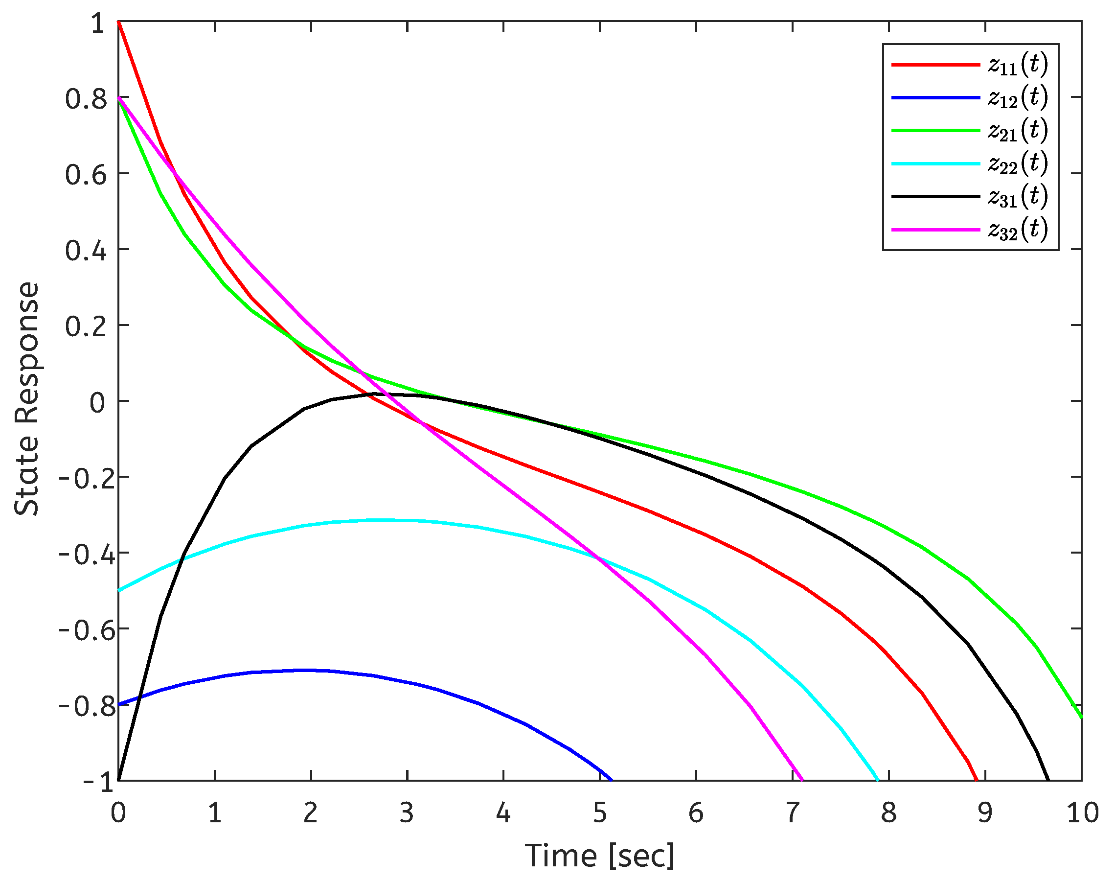
4. Simulation Results

In this section, a numerical example will be presented to illustrate the effectiveness of the theoretical analysis.

Consider system (1) with $n=2$ and $N=3$, the parameter matrices are given [14,34] $A=\left[\begin{array}{ccc}-1& 0& 1\\ 0& -1& 0\\ 1& 1& 2\end{array}\right]$, $B=\left[\begin{array}{cc}1& 0\\ 0& 1\end{array}\right]$. and nonlinear function

$$\begin{array}{c}\hfill f\left(x_i\left(t\right)\right))=\left[\begin{array}{c}-0.5x_{i1}\left(t\right)+tanh\left(0.2x_{i1}\left(t\right)\right)+0.2x_{i2}\left(t\right)\\ 0.9x_{i2}\left(t\right)-tanh\left(0.75x_{i2}\left(t\right)\right)\end{array}\right].\end{array}$$

Then, we can obtain

$$\begin{array}{c}\hfill L_1=\left[\begin{array}{cc}-0.3& 0.2\\ 0& 0.2\end{array}\right],L_2=\left[\begin{array}{cc}-0.5& 0.2\\ 0& 0.95\end{array}\right]\end{array}$$

Taking the coupling strength $c=0.2$, $u_{0il}=1$, and $\mu =0.1$. By solving Theorem 2, we can obtain $h=0.5881$ and

$$\begin{array}{cc}& K_{11}=\left[\begin{array}{cc}-0.4905& 0.8800\\ -0.4496& 0.4575\end{array}\right],K_{12}=\left[\begin{array}{cc}-0.5786& -0.0464\\ -0.6810& -0.0883\end{array}\right]\hfill \\ & K_{13}=\left[\begin{array}{cc}-0.5786& -0.0464\\ -0.6810& -0.0883\end{array}\right],K_{21}=\left[\begin{array}{cc}-0.4905& 0.8800\\ -0.4496& 0.4575\end{array}\right]\hfill \\ & K_{22}=\left[\begin{array}{cc}-0.5786& -0.0464\\ -0.6810& -0.0883\end{array}\right],K_{23}=\left[\begin{array}{cc}-0.5786& -0.0464\\ -0.6810& -0.0883\end{array}\right].\hfill \end{array}$$

and, the largest BoA can be calculated as

$$\begin{array}{cc}& \mathfrak{E}=\left\{z\left(t_0\right)\in {\mathbb{R}}^6\mid 0.0323\underset{-0.1\le s\le 0}{sup}\{\parallel z\left(s\right){\parallel }^2,\parallel \dot{z}\left(s\right){\parallel }^2\}\le 1\right\}.\hfill \end{array}$$

The initial conditions are set as $x\left(t_0\right)={[3,-5;4,-3;-4,-2]}^T$ and $y\left(0\right)={[2,-1]}^T$. When $u_i=0$, the state response of the open-loop error system is shown in Figure 1. The state response of the closed-loop system is shown in Figure 2. It can be seen from Figure 2 that the local stabilization of the error system (6) can be achieved, which indicates that the CDNs (1) and isolated node (2) are exponentially synchronized under the controller (4). Figure 3 depicts the curves of the control input $u_i\left(t\right)$, and the aperiodic sampling interval for the initial state.

5. Conclusions

In this paper, based on SDC, the issue of exponential synchronization control for CDNs with input saturation has been studied. Considering the impact of transmission delay $\mu$, a design method for a memory sampled-data controller has been proposed. By constructing an improved two-sided looped functional that includes both current state information and delayed state information, where both $z(t_{\kappa }-\mu )$ and $z(t_{\kappa +1}-\mu )$ have been considered, and combining it with inequality techniques, the criteria for ensuring the local stability of the closed-loop system have been provided. Meanwhile, under the influence of transmission delay, an estimation of the BoA for the initial values has been given, along with an optimization algorithm to enlarge it. Finally, a numerical example has been presented to verify the effectiveness of the results. Due to the susceptibility of complex network environments to external attacks, the question of how to achieve effective anti-attack security control under different types of attacks is a topic worthy of future research.

References

1. Strogatz, S.H. Exploring complex networks. Nature 2001, 410, 268–276. [Google Scholar] [CrossRef]
2. Albert, R.; DasGupta, B.; Mobasheri, N. Topological implications of negative curvature for biological and social networks. Phys. Rev. E 2014, 89, 032811. [Google Scholar] [CrossRef] [PubMed]
3. Rampurkar, V.; Pentayya, P.; Mangalvedekar, H.A.; Kazi, F. Cascading failure analysis for Indian power grid. IEEE Trans. Smart Grid 2016, 7, 1951–1960. [Google Scholar] [CrossRef]
4. Guo, R.; Xu, S.; Zhang, B.; Ma, Q. Nonfragile Exponential Synchronization for Delayed Fuzzy Memristive Inertial Neural Networks via Memory Sampled-Data Control. IEEE Trans. Fuzzy Syst. 2024, 32, 3825–3837. [Google Scholar] [CrossRef]
5. Liu, D.; Ye, D. Edge-based decentralized adaptive pinning synchronization of complex networks under link attacks. IEEE Trans. Neural Netw. Learn. Syst. 2022, 33, 4815–4825. [Google Scholar] [CrossRef]
6. Tan, F.; Zhou, L.; Lu, J.; Chu, Y.; Li, Y. Fixed-time outer synchronization under double-layered multiplex networks with hybrid links and time-varying delays via delayed feedback control. Asian J. Control 2022, 24, 137–148. [Google Scholar] [CrossRef]
7. Wu, Y.; Li, Y.; Li, W. Synchronization of random coupling delayed complex networks with random and adaptive coupling strength. Nonlinear Dyn. 2019, 96, 2393–2412. [Google Scholar] [CrossRef]
8. Zhang, W.; Li, H.; Li, C.; Li, Z.; Yang, X. Fixed-time synchronization criteria for complex networks via quantized pinning control. ISA Trans. 2019, 91, 151–156. [Google Scholar] [CrossRef]
9. Liu, X.; Chen, T. Synchronization of complex networks via aperiodically intermittent pinning control. IEEE Trans. Autom. Control 2015, 60, 3316–3321. [Google Scholar] [CrossRef]
10. Wang, L.; Zhang, C.K. Exponential synchronization of memristor-based competitive neural networks with reaction-diffusions and infinite distributed delays. IEEE Trans. Neural Netw. Learn. Syst. 2024, 35, 745–758. [Google Scholar] [CrossRef]
11. Hu, X.; Wang, L.; Zhang, C.K.; He, Y. Fixed-time synchronization of fuzzy complex dynamical networks with reaction-diffusion terms via intermittent pinning control. IEEE Trans. Fuzzy Syst. 2024, 32, 2307–2317. [Google Scholar] [CrossRef]
12. Li, Y.; Lu, J.; Alofi, A.S.; Lou, J. Impulsive cluster synchronization for complex dynamical networks with packet loss and parameters mismatch. Appl. Math. Model. 2022, 112, 215–223. [Google Scholar] [CrossRef]
13. He, S.; Wu, Y.; Li, Y. Finite-time synchronization of input delay complex networks via non-fragile controller. J. Frankl. Inst. 2020, 357, 11645–11667. [Google Scholar] [CrossRef]
14. Liu, Y.; Guo, B.; Park, J.H.; Lee, S. Nonfragile exponential synchronization of delayed complex dynamical networks with memory sampled-data control. IEEE Trans. Neural Netw. Learn. Syst. 2018, 29, 118–128. [Google Scholar] [CrossRef]
15. Zhao, C.; Zhong, S.; Zhang, X.; Zhong, Q.; Shi, K. Novel results on nonfragile sampled-data exponential synchronization for delayed complex dynamical networks. Int. J. Robust Nonlinear Control 2020, 30, 4022–4042. [Google Scholar] [CrossRef]
16. Zhang, R.; Zeng, D.; Park, J.H.; Liu, Y.; Zhong, S. Nonfragile sampled-data synchronization for delayed complex dynamical networks with randomly occurring controller gain fluctuations. IEEE Trans. Syst. Man Cybern. Syst. 2018, 48, 2271–2281. [Google Scholar] [CrossRef]
17. Huang, X.; Cao, X.; Ma, Y. Sampled-data exponential synchronization of complex dynamical networks with time-varying delays and T–S fuzzy nodes. Comput. Appl. Math. 2022, 41, 74. [Google Scholar] [CrossRef]
18. Wen, G.; Yu, W.; Chen, M.Z.Q.; Yu, X.; Chen, G. H-pinning synchronization of directed networks with aperiodic sampled-data communications. IEEE Trans. Circuits Syst. I Reg. Pap. 2014, 61, 3245–3254. [Google Scholar] [CrossRef]
19. Song, X.; Zhang, R.; Ahn, C.K.; Song, S. Synchronization for semi-markovian jumping reaction-diffusion complex dynamical networks: A space-time sampled-data control scheme. IEEE Trans. Netw. Sci. Eng. 2022, 9, 4. [Google Scholar] [CrossRef]
20. Gunasekaran, N.; Ali, M.S.; Arik, S.; Ghaffar, H.A.; Diab, A.A.Z. Finite-time and sampled-data synchronization of complex dynamical networks subject to average dwell-time switching signal. Neural Netw. 2022, 149, 137–145. [Google Scholar] [CrossRef]
21. Hu, T.; Park, J.H.; Liu, X.; He, Z.; Zhong, S. Sampled-data-based event-triggered synchronization strategy for fractional and impulsive complex networks with switching topologies and time-varying delay. IEEE Trans. Syst. Man Cybern. Syst. 2022, 52, 3568–3578. [Google Scholar] [CrossRef]
22. Huang, Y.; Bao, H. Master-slave synchronization of complex-valued delayed chaotic Lur’e systems with sampled-data control. Appl. Math. Comput. 2020, 379, 125261. [Google Scholar] [CrossRef]
23. Seuret, A. A novel stability analysis of linear systems under asynchronous samplings. Automatica 2012, 48, 177–182. [Google Scholar] [CrossRef]
24. Zeng, H.; Teo, K.L.; He, Y. A new looped-functional for stability analysis of sampled-data systems. Automatica 2017, 82, 328–331. [Google Scholar] [CrossRef]
25. Zeng, H.; Zhai, Z.; He, Y.; Teo, K.; Wang, W. New insights on stability of sampled-data systems with time-delay. Appl. Math. Comput. 2020, 374, 125041. [Google Scholar] [CrossRef]
26. Stein, G. Respect the unstable. IEEE Control Syst. 2003, 23, 12–25. [Google Scholar]
27. Chen, Y.; Wang, Z.; Shen, B.; Dong, H. Exponential synchronization for delayed dynamical networks via intermittent control: Dealing with actuator saturations. IEEE Trans. Neural Netw. Learn. Syst. 2019, 30, 1000–1012. [Google Scholar] [CrossRef] [PubMed]
28. Chen, Y.; Wang, Z.; Hu, J.; Han, Q.-L. Synchronization control for discrete-time-delayed dynamical networks with switching topology under actuator saturations. IEEE Trans. Neural Netw. Learn. Syst. 2021, 32, 2040–2053. [Google Scholar] [CrossRef]
29. Wu, Y.; Su, H.; Wu, Z. Synchronization control of dynamical networks subject to variable sampling and actuators saturation. IET Control Theory Appl. 2015, 9, 381–391. [Google Scholar] [CrossRef]
30. Chen, G.; Xia, J.; Park, J.H.; Shen, H.; Zhuang, G. Robust sampled-data control for switched complex dynamical networks with actuators saturation. IEEE Trans. Cybern. 2022, 52, 10909–10923. [Google Scholar] [CrossRef]
31. Zhou, H.; Liu, Z.; Li, W. Sampled-data intermittent synchronization of complex-valued complex network with actuator saturations. Nonlinear Dyn. 2022, 107, 1023–1047. [Google Scholar] [CrossRef]
32. Seuret, A.; Gouaisbaut, F. Wirtinger-based integral inequality: Application to time-delay systems. Automatica 2013, 49, 2860–2866. [Google Scholar] [CrossRef]
33. Zhang, X.; Han, Q.; Seuret, A.; Gouaisbaut, F. An improved reciprocally convex inequality and an augmented Lyapunov-Krasovskii functional for stability of linear systems with time-varying delay. Automatica 2017, 84, 221–226. [Google Scholar] [CrossRef]
34. Wu, Z.-G.; Shi, P.; Su, H.; Chu, J. Sampled-data exponential synchronization of complex dynamical networks with time-varying coupling delay. IEEE Trans. Neural Netw. Learn. Syst. 2013, 24, 1177–1187. [Google Scholar]
Figure 1. State trajectory of the error system without controller.
Entropy 26 00785 g001
Figure 2. State response of the closed-loop system.
Entropy 26 00785 g002
Figure 3. Control inputs and aperiodic sampled-data interval.
Entropy 26 00785 g003
Disclaimer/Publisher’s Note: The statements, opinions and data contained in all publications are solely those of the individual author(s) and contributor(s) and not of MDPI and/or the editor(s). MDPI and/or the editor(s) disclaim responsibility for any injury to people or property resulting from any ideas, methods, instructions or products referred to in the content.