Abstract
Radical pair kinetics is determined by the coherent and incoherent spin dynamics of spin pair and spin-selective chemical reactions. In a previous paper, reaction control and nuclear spin state selection by designed radiofrequency (RF) magnetic resonance was proposed. Here, we present two novel types of reaction control calculated by the local optimization method. One is anisotropic reaction control and the other is coherent path control. In both cases, the weighting parameters for the target states play an important role in the optimizing of the RF field. In the anisotropic control of radical pairs, the weighting parameters play an important role in the selection of the sub-ensemble. In coherent control, one can set the parameters for the intermediate states, and it is possible to specify the path to reach a final state by adjusting the weighting parameters. The global optimization of the weighting parameters for coherent control has been studied. These manifest calculations show the possibility of controlling the chemical reactions of radical pair intermediates in different ways.
1. Introduction
A radical pair (RP) is composed of two radicals, each of which has an unpaired electron. When RPs are produced photochemically, the initial electron spin state of the RPs preserves the spin manifold of the precursor excited state. Although this fact has been known for a long time, it has been re-evaluated and has attracted much attention because this state is the so-called “entanglement state” [1,2,3,4,5]. On the other hand, the formation of RPs is also known in photoreceptor protein systems, such as photosynthetic reaction centers [6,7,8,9] and cryptochromes (CRYs) [10,11,12,13,14]. In particular, CRYs are candidate molecules for magnetoreception in animals, and the relationship between magnetism and biological systems has been discussed [15,16,17,18,19]. The influence of not only magnetic fields but also that of electromagnetic waves has been discussed [20]. In the geomagnetic perception of migratory birds, the influence of electromagnetic noise is still under discussion [21].
The most probable effect of electromagnetic waves on RPs is magnetic resonance [22]. It is called reaction yield detected magnetic resonance (RYDMR) [23,24,25,26,27,28,29] and is measured at different external magnetic fields and resonance frequencies. Figure 1 shows a schematic diagram of the spin state and chemical reactivity of RPs. Here, we consider the typical case where a singlet-born radical pair reacts spin-selectively from the singlet state under the magnetic field. At the high magnetic field, the microwave frequency matching with the Zeeman splitting energy induces the resonance phenomena, producing and states, which do not have singlet properties and are retained for a long time or become free radicals by radical diffusion. Therefore, recombination reactions from the singlet state are significantly suppressed by the magnetic resonance phenomena. On the other hand, in a small magnetic field at the geomagnetic level, Zeeman splitting is smaller than hyperfine coupling, so the resonance of the radiofrequency to hyperfine coupling is important. Such magnetic resonance phenomena of RPs are complex, but the resulting change in the singlet character of RPs affects the reaction yield. In contrast to Figure 1, the spin states of general RPs are more complex. The resonance frequency of RPs is the same as the electron spin resonance frequency of the two constituent radicals when the interaction between the radicals is negligibly small. However, they are complicatedly split by hyperfine coupling and its anisotropy. If high-field approximation holds and mixing between the nuclear spin states is small, these resonance lines can be considered as sub-ensembles. In such a case, the selection of these sub-ensembles can be conducted by selecting the RF frequency.
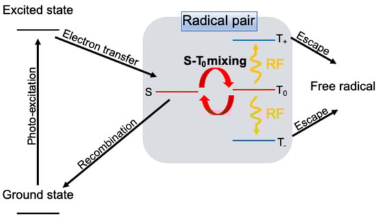
Figure 1.
Reaction scheme for the formation of singlet RPs, and reactivity control by RF transitions (RYDMR).
The spin states of a radical pair can be regarded as a quantum mechanical system. Therefore, the control of chemical reactions associated with the spin manipulation of RPs is said to be a quantum state manipulation. In the field of magnetic resonance, an optimization technique called GRAPE (Gradient Ascent Pulse Engineering) [30] is widely used. GRAPE optimizes the waveform globally on the time axis, but it tends to be trapped in local optimal states due to the combination of many segments of the RF field. In this sense, it is not a perfect global optimization for multiple variables. Therefore, in many cases, it is necessary to set many waveforms as initial conditions to find the global optimal waveform, which inevitably increases the computational complexity. Therefore, the application of this method is limited to a small number of short pulse designs and is difficult to optimize the RF field for the chemical reaction control to occur over long periods of time.
On the other hand, a local optimization method with respect to the time axis has been used to design an infrared laser field for vibronic state control [31]. This method works very well for relatively simple quantum states and the optimal wave can be obtained in a very short computation time. In contrast to the GRAPE method, this method requires essentially no iterative computation. Thus, the optimized waveform and the resulting time evolution of the system are obtained simultaneously in a single calculation. The method is based on the concept of “living for the day” and monotonically increases fidelity, i.e., the overlap of the system with the target state. In fact, although it is a very crude method, it shows excellent results for quantum systems achieved with relatively simple paths.
We have applied this local optimization method to control the chemical reaction of RPs. This method has the following features:
- (1)
- Smooth waveforms can be obtained because waveforms can be computed with very high time resolution. In contrast, the waveforms computed in GRAPE are optimized for relatively coarse time steps.
- (2)
- Sub-ensemble systems can be easily selected by resonance frequency in inhomogeneous RP systems.
- (3)
- The calculation can incorporate strategies for the time evolution of the quantum system with respect to its path.
- (4)
- Calculations in a rotational coordinate system are easy because there is no computational burden due to the multidimensionality of radio waves (microwaves).
In particular, sub-ensemble selection (2) and path control in coherent control (3) can be achieved by using the same sets of parameters, called weighting parameters {}, which will be discussed in the next section. In a previous paper [32], we demonstrated (2) nuclear spin state selections under (3) high-field approximation. In the present paper, we present anisotropic reaction control and coherent control in an extremely low magnetic field, focusing on the weighting parameters. Furthermore, we have improved the local-optimization-based coherent control of the spin system of RPs via the global optimization of a few weighting parameters. Of course, this method is not perfect global optimization, but it is a significant improvement. The model system used here is rather simple compared to realistic systems. However, once the methodology is developed and a strategy for reaction control is established, it should be easy to apply them to a realistic system because the computational burden is significantly lower.
2. Theory
We have previously applied the local optimization theory, which was used for the control of vibronic systems using an infrared laser [31], to the design of RF magnetic field for the control of RP chemical reactions [32]. In order to extend computational flexibility and to take into account spin-selective chemical reactions and spin relaxations, the basic theory of the local optimization theory has been reformulated in Liouville space. In this chapter, we provide an overview of the theory and describe the important weighting parameters in control. Then, anisotropic control and coherent pathway control are formulated as an example of control using weighting parameters.
2.1. Local Optimization Theory
We begin with an overview of the local optimization theory for our reaction control [31,32]. In the local optimization theory, the degree of achievement of a desired quantum state is set as a performance index, and control is realized by designing an external oscillating field such that the performance index increases monotonically. Defining as the projection operator of the target quantum state (where considers eigenstates of system Hamiltonian but can be extended to non-eigenstates), the performance index is described as follows.
is the density matrix of the system, and its time evolution follows the Liouville von Neuman equation in Liouville space.
where is composed of the static term, , which drives the time evolution by the static Hamiltonian , and time dependent term,
, which represents the interaction with the optimized oscillating RF fields :
where hat and tilde denote the operation to ket and bra in Hilbert spaces, respectively.
From , the time derivative of the performance index is written by:
Now, we introduce an amplitude parameter , which determines the degree of optimization as well as the weighting parameter, which will be discussed later, and if is given by
a monotonical increase in is guaranteed.
Substituting Equation (5) into Equation (2), we obtain the nonlinear differential equation shown in Equation (7).
Once we solve the time evolution of , we can obtain by Equation (5).
2.2. Weighting Parameters
Equation (1) was an evaluation function of control targeting a single quantum state, but to target multiple quantum states, we extend Equation (1) as follows.
Here, we introduce the weighting parameters , which determine the priority to the target states . They are useful for the following two types of control.
One is sub-ensemble control, in which each sub-ensemble, such as different nuclear spin configurations under a high field approximation, isotope selection, and any inhomogeneous spectral broadening of the spin systems. Here, we focus on the orientation of an anisotropic system with respect to laboratory coordinates. By setting weighting parameters for each sub-ensemble, it is possible to induce () or suppress () transitions only in certain sub-ensembles.
The other is path control. By setting the weighting parameters for the quantum states , transitions can occur in the order . In other words, these parameters can be thought of as guiding the transition path to produce a particular spin state at a particular time. From the next chapter, we will formulate these controls in a radical pair system.
2.3. Anisotropic Sub-Ensemble Control
Here, we consider RPs with an anisotropic hyperfine interaction. The sub-ensemble can be determined by the orientation with respect to the laboratory coordinates. The Hamiltonian of the anisotropic hyperfine interaction is described as follows.
The operators and correspond to the electron and nucleus spin operators, respectively, and is a hyperfine tensor. is diagonalized by multiplying the appropriate rotation matrix:
The subscripts correspond to in the molecular coordinate system. To describe the anisotropic response of a molecule to the direction of a static magnetic field , the molecular coordinate system needs to be transformed into a laboratory frame. The orientation of these two coordinates systems is defined by the following Euler angles as shown in Figure 2. The conversion of the coordinates can be described by a rotational matrix :
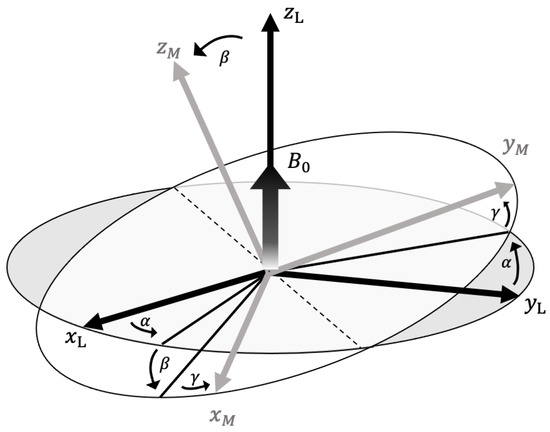
Figure 2.
The relationship between molecular frame () and laboratory frame () defined by Euler angles (). is defined to be parallel to .
By using , the hyperfine tensor in laboratory frame can be calculated by:
Here, we introduce the new index for the sub-ensembles of RPs. The Hamiltonian of a radical pair with one nuclear spin () for a sub-ensemble is given by:
The first and second terms correspond to the electron spin Zeeman interaction of radical A and radical B, the third term indicates the nuclear Zeeman interaction, the fourth term denotes the hyperfine interaction, and the fifth term represents the exchange interaction of the RPs.
Since the index represents the sub-ensemble of orientations relative to the magnetic field direction of the system, the total density vector can be divided into the vector for each sub-ensemble . Thus, the performance index can be defined by:
is the projection operator for the target states, and is the weighting factor for . is the product of the weighting factor and the Jacobian (). The can be constructed as follows:
- The eigenstates of were calculated.
- The two eigenstates with the largest and characteristics were chosen, where the state and indicate electron spin state with α nuclear spin and with β nuclear spin, respectively.
- The sum of the projection operators onto these two eigenstates was determined to be the target, .
The magnetic resonance transitions from the singlet rich eigenstates to the target steady states increase and provide long-lived RP sub-ensembles. By an appropriate setting of the weighting parameters, one can select the specific sub-ensembles and transfer the population to the stable eigenstates that are free from the recombination reaction.
The kinetics of the RPs reaction of each sub-ensemble can be calculated by the Haberkorn super operator, using the projection operator [33,34,35].
Since , occasionally decreases by the recombination kinetics. Therefore, this calculation is limited to the condition where is much smaller than the frequency of spin dynamics. In this model calculation, we have set , such that the introduction of recombination reactions has a minimal effect on the optimized waveforms and does not break down the calculation.
The calculation process of anisotropic reaction control is performed in the same way as the previous calculation, i.e., solving the Liouville von Neuman equation, Equation (17) using optimized , which guarantees a monotonous increase in :
2.4. Coherent Pathway Control
In coherent control, the non-eigenstate of the Hamiltonian is set as the target state. Since the non-eigenstate evolves automatically in time, the target state should be set at a specific time , and reverse time evolution should be introduced.
where is a Liouvillian of field-free Hamiltonian . We call this time-dependent target state the moving target. If the density vector of the system can be reached to the moving target by applying the external field at time , the desired state can be obtained automatically at time . In a magnetic field, the singlet state becomes an unsteady state due to S-T0 mixing. Therefore, the singlet state is a candidate for the target of coherent control. If the singlet state can be maximized at , a spin-selective reaction, such as a recombination reaction, can be promoted. However, depending on the target state, it may be difficult to directly reach the moving target. Even in such a case, the moving target can be obtained by introducing the intermediate state and the weighting factor [36].
Here, the roles of are not the same as in Section 2.3, but are rather parameters for specifying the transition path. By setting , it becomes possible to specify a transition path that transitions to the state at time via the state . In such a way, one can input strategies into the spin dynamics of RPs.
To evaluate the degree of achievement of , the performance index is defined as:
The time evolution of is described by the Liouville von Neuman equation, so the time derivative of is given by:
As in previous discussions, by defining as Equation (22), a monotonous increase in Equation (20) is guaranteed (Equation (23)).
As a result, the equation that the coherent controlled system follows is following a nonlinear differential equation.
In the coherent control calculations, we assume a single nuclear spin as in the anisotropy calculations. However, we consider only isotropic hyperfine coupling. The spin Hamiltonian is given by:
In addition, for coherent control, we did not consider the recombination reaction.
2.5. Parameter Global Optimization
The parameters used for control, such as the weighting parameter . and the amplitude parameter , have a strong influence on the fidelity of the desired quantum state depending on their values. To obtain the desired state with high fidelity, it is necessary to use an appropriate combination of parameters. Therefore, we define the fidelity of the target state obtained by the one control as a function of and , Equation (26), and use global optimization (ga function in MATLAB Global Optimization Toolbox [37,38,39]) to find the combination of parameters that maximizes the fidelity of .
While global optimization requires iterative computations and is computationally expensive, it is more likely to obtain the desired parameters without being trapped by a local minimum due to its holistic search. In contrast, computations based on the local optimization theory do not require iterative computations, so the one-time computational cost is very low and practical control results can be obtained, but whether the obtained results are the best results cannot be determined in a single computation. Therefore, a global search of the parameters necessary for local optimization is a good method that combines the advantages of both local and global optimization since it can calculate optimal values while reducing the computational cost of each iteration of the search. Using this method, the optimal parameters for coherent control were obtained ( described below, which was obtained by this method).
3. Results and Discussion
3.1. Anisotropic Reaction Control
Model RPs g-factors are set as , and external magnetic field was fixed to 3.6 mT. The following anisotropic hyperfine tensor was used.
The exchange interaction was fixed to 0.1 MHz. The initial state of RP is assumed to be singlet state.
First, we designed a waveform that provides a transfer of the radical pair from S-T0 mixed states to states homogeneously. This control corresponds with keeping the RP population isotropic in the magnetic field direction by setting for all . Figure 3 shows the results of the optimized RF field and decay of RPs with and without RF.
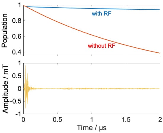
Figure 3.
(Upper) Time evolution of model RP’s population (blue line: with RF, red line: without RF). (Lower) calculated RF field.
Figure 3 shows that 2 s after radical pair formation, the population of RPs, which is 38% in the case of no RF irradiation, is successfully maintained at 94% by RF irradiation. This is a result of the RF-induced transition of the radical pair from the singlet to states with high and character, which are hardly involved in S-T0 mixing, and the suppression of the recombination reaction.
We now examine the anisotropy of the RP population using the coordinates shown in the top panel of Figure 4. Figure 4 shows the RP population at = 2 s during RF irradiation and non-irradiation, indicating that the RP population is maintained isotropically during RF irradiation.
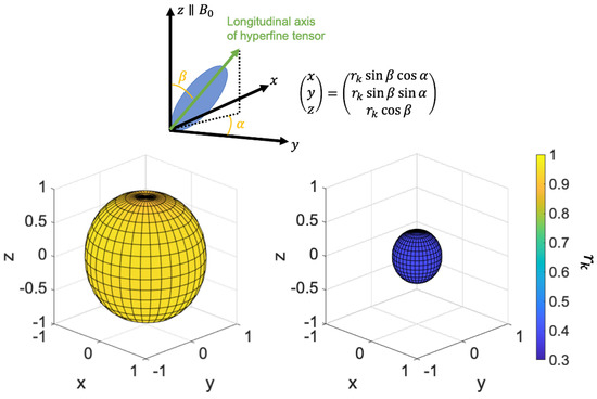
Figure 4.
(Upper) Correspondence between the long axis direction of the hyperfine tensor and the coordinates (x, y, z). The length and color of represents RP’s population. Notation of angles is consistent with Figure 2. (Lower) RP population (t = 2 μs) with RF (left), without RF (right).
Figure 5 shows the results of a Fourier transform of the irradiated RF signals, and it can be confirmed that the frequency components corresponding to the transitions of radical B are dominant. This is because the transition to radical B, which has isotropic interactions, is advantageous for maintaining an isotropic population.
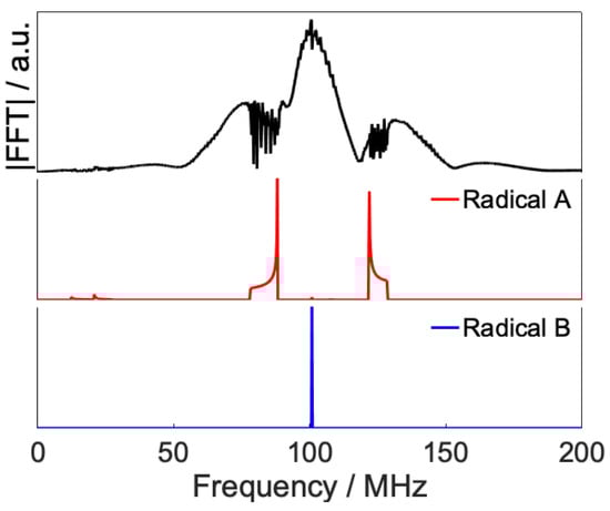
Figure 5.
Fourier transform of calculated radio waveform (Figure 3) and simulation results of frequency swept powder ESR spectrum of the model RP calculated by an Easy Spin package (Pepper) with minimum line width.
From now on, we consider the control of the RP population anisotropic with respect to the external static magnetic field direction (). At first, we tried to keep the RPs with nearly parallel orientation with respect to the external field, i.e., . We set for = 0~50°, 130~180°, and for = 60~120°. The negative value directly means a penalty for the undesired transition.
Figure 6 shows the results of the anisotropic control. The RP population decays by recombination for sub-ensembles 60~120° and the component, for = 0~50°, 130~180° stayed longer as RPs. This is because the RF-induced transitions to the eigenstates with relatively high and character for the sub-ensemble = 0~50°, 130~180° remarkably suppress the recombination efficiency, while the recombination was not suppressed for the sub-ensemble of = 60~120° because the transitions were not induced.
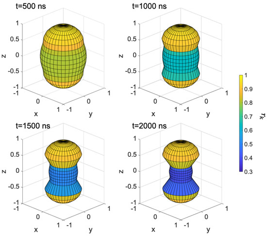
Figure 6.
Time evolution of the anisotropic control to retain when the RPs whose longitudinal axis of hyperfine tensor is nearly parallel to the magnetic field is held.
The Fourier transform of the optimized waveform is shown in Figure 7. In contrast to the isotropic control case, the algorithm for the optimized waveform has switched the target radical transition from radical B to radical A, because radical A has the frequency distribution of the transition due to the anisotropic hyperfine interaction.
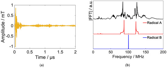
Figure 7.
(a) Optimized RF field for anisotropic control. (b) Fourier transform of (a) and simulated frequency swept powder ESR spectrum of model RP.
Next, we tried to keep the RPs of the = 60~120° sub-ensemble longer. For this, the time weighting parameters were set to for = 0~50°, 130~180° sub-ensemble and for the = 60~120° sub-ensemble.
In contrast to the previous result, RPs whose hyperfine tensors are relatively oriented perpendicular to the magnetic field direction are retained, while RPs whose hyperfine tensors are oriented parallel to the magnetic field direction are reduced, as shown in Figure 8. Figure 9 shows the optimized waveform and the result of the Fourier transform. The frequency components corresponding to the transitions of radical A tend to dominate, but the components corresponding to the transitions of radical B are increased compared to the previous control. In order to confirm the timing of the frequency components used in the control, we performed short-time Fourier transform, as shown in Figure 10.
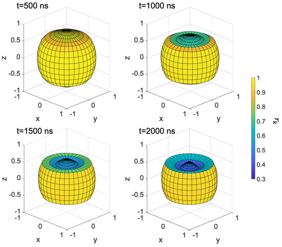
Figure 8.
Time evolution of the anisotropic control to retain RPs whose longitudinal axis of hyperfine tensor is relatively perpendicular to the magnetic field.
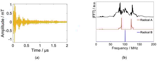
Figure 9.
(a) Optimized RF field. (b) Fourier transform of (a) and simulation results of frequency swept powder ESR spectrum of model RP.
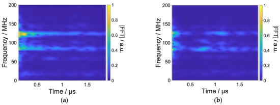
Figure 10 shows that the frequency components of radical A are used for a long time in both the controls shown in Figure 6 and Figure 8, while the frequency components of radical B are used only in the early time (see around 100 MHz). In the early stage, the transition to radical B contributes to the total RPs being maintained for a longer time, thus contributing to the increase in the performance index . On the other hand, in the later part, isotropic transitions to radical B are avoided in order to avoid an increase in the sub-ensemble with penalized weighting parameters.
Our calculation can increase the performance index by selecting the RF frequency precisely over a long period of time, ~2 μs. In practice, however, most of the control is achieved relatively early. In the three examples shown in Figure 3, Figure 7 and Figure 9, the performance index y(t) at t = 0.25 μs is 97%, 79%, and 92% of y(t) at t = 2 μs, respectively.
3.2. Coherent Pathway Control
Now, we discuss coherent control. For coherent control, the hyperfine coupling constant was set to 15 MHz (0.54 mT), the RP’s g-factors were set as , and the exchange interaction was set to 0.1 MHz. Under this condition, only the hyperfine interaction contributes to S-T0 mixing. The calculation was performed under external magnetic fields of 20 mT and 0.05 mT. As in the previous section, the initial state of the RP was set to the singlet state, and the calculation was performed so that the RP returned to the singlet state again after 1 s via the T± state. To handle this control, the moving target was set as Equation (28).
Figure 11 shows the result of coherent control under .
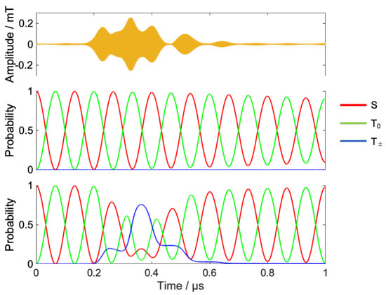
Figure 11.
Results of the coherent control under 20 mT. Optimized RF (upper), time evolution of spin state without RF (middle), and with RF (lower).
In the high-field condition, the time evolution does not produce the probability of T±. Therefore, the strategy of coherent control is as follows.
- S-T0 mixing increases the population of T0 states;
- The RF provides a transition from the T0 state to the T± state;
- The transition from T± to T0 is again triggered by the RF, timed to maximize the singlet at the target time.
The population of the singlet state after 1s without RF irradiation is less than 10% due to S-T0 mixing. Optimized RF induces T0 – T± transitions around 0.2s, and the subsequent T± − T0 transition shifts the phase of S-T0 mixing, eventually returning about 98% of the RP to the singlet state at 1 s.
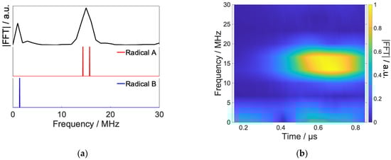
Figure 12a,b show the power spectrum of the optimized RF and short-time Fourier transform, respectively. The optimized RF is mainly composed of radical B, which has no hyperfine interaction. The peak of this frequency component rises from 0.2 s and decays around 0.6 s, which is in good agreement with the time evolution of the spin state. From these results, we can confirm that the local control theory has attained the desired control by causing transitions to the radical B step by step in the control at a high magnetic field.
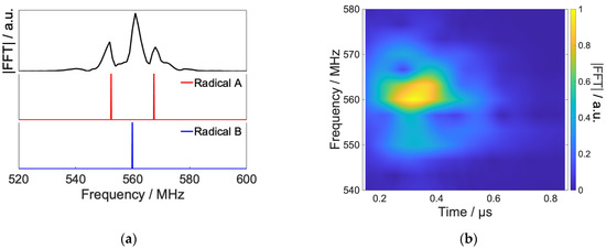
Figure 12.
Spectrum of the calculated RF field by Fourier transform and simulation results of frequency swept ESR spectrum of model RP (a) and short-time Fourier transform of radio waves in Figure 11 (b). The Hanning window is used as the window function, and the length of the window function is 300 ns with a hop size of 10 ns.
In the extremely low magnetic field condition ( = 0.05 mT), the energy separation Zeeman splitting becomes small, and hyperfine interactions dominate. As a result, not only S-T0 mixing but also other state mixings occur, as shown in Figure 13. The mixing between spin states looks more complicated than at 20 mT. In the model system, singlet states mix with , but states remain isolated even in a low magnetic field. Only the RF field can make transitions to the isolated . Therefore, these states are useful as the intermediate quantum states for the coherent control of the RPs. To achieve more efficient population control, the moving target with weighting factors for was employed.
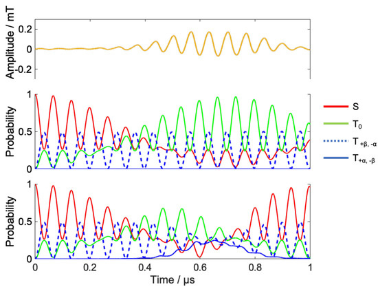
Figure 13.
Results of the coherent control under 0.05 mT. Optimized RF (upper), time evolution of spin state without RF (middle), and with RF (lower).
Figure 13 shows the result of coherent control under . By optimized RF, RP’s population were stored to states for 0.4 s to 0.9 s. Due to the transitions, the phase of S-T0 mixing was changed around 0.5 s, and singlet fidelity was improved from 39% to 96%.
Figure 14 shows the power spectrum and the short-time Fourier transform of optimized RF shown Figure 13. In contrast to the high field case, the frequency component corresponding to the transition of radical A mainly constitutes optimized RF. This is considered because the Zeeman splitting under the geomagnetic field is so small that the RF prioritizes the control of transitions between states split by nuclear spins. Thus, under very low magnetic fields such as the geomagnetic field, the broad frequency component due to the hyperfine interaction of the system can affect the reaction rather than the Zeeman splitting of the external magnetic field [21], and the present control results suggest this.
3.3. Parameter Optimization
Figure 15 shows the evolution of the weighting parameters and amplitude parameter A and Singlet fidelity at the target time (1 s) during global optimization.
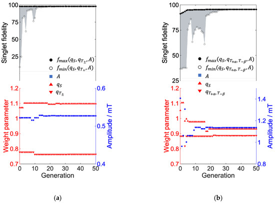
Figure 15.
Fidelity of singlet of coherent control and evolution of each parameter value when optimized with ga function of global optimization ((a): high field control of Figure 11, (b): geomagnetic field control of Figure 13). Generation indicates the number of iterations in Global optimization, where 50 parameter combinations are computed in one generation. The parameters search range was set to . and indicate highest and lowest value of the singlet yield in each generation, and the singlet fidelity values for each generation are distributed in the gray area.
At generation zero, we set arbitrary weighting parameters and amplitude parameters. The genetic algorithm (ga function) of the MATLAB global optimization toolbox generated fifty sets of parameters {} and calculated the locally optimized RF field. In fifty sets of the calculations, the maximum and minimum fidelities, and , were plotted as shown in Figure 15. This process was repeated fifty times and we can confirm the convergence of the fidelities with respect to the parameter sets. As shown in Figure 15, the number of generations required for the convergence of the parameter sets is greater for the low-field control (Figure 15b) than for the high-field control (Figure 15a). The high field control is a simple problem of how to make a phase shift of S-T0 mixing oscillating by a single frequency. In contrast, the control at a low magnetic field is more difficult because the coherent oscillations contain both the hyperfine coupling and the external magnetic field, and the value of the control parameter has a large effect on the fidelity of the singlet. Therefore, the high-field results converged early, while the low-field results required more generations to converge the parameters. Here, we define as the parameter combination , which provides the maximum value of singlet fidelity and as the parameter combination , which provides the minimum value of singlet fidelity in low-magnetic-field control.
Figure 16 shows the time evolution of the spin system when and are used as control parameters. The transition to the state is slower in the control using compared to the control using , and the target time is reached before the RP populations return to singlet state again. This reflects the importance of the optimal combination of parameters, especially when coherent mixing is significant. Therefore, the global search for local optimization parameters used in this study is a method that can compensate for the weakness of the local optimization method and obtain better control results.
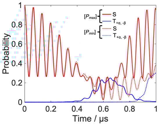
Figure 16.
Time evolution of spin systems under low field control when and (see the text for details) are used as parameters. (solid line: control result using , dotted line: control result using ).
4. Concluding Remarks
In this paper, we focused on the weighting parameters used to control local optimization and demonstrated sub-ensemble and coherent control for a model system of RPs. By using appropriate weighting parameters, we achieved control over the selection of anisotropic sub-ensembles and the design of transition paths, albeit in a simple system.
The anisotropic response of RPs to magnetic fields is of interest from the perspective of avian magnetic compasses, and the possibility of oscillating magnetic fields affecting their dynamics is related to test experiments on animal behavior. The anisotropic induction of RP by RF irradiation presented in this paper, together with the fact that broadband RF irradiation disrupts the orientation of migratory birds [15,20,21], implies that RF irradiation of a certain waveform may be able to induce bird orientation. However, in practice, it would be difficult to apply this method to animal experiments in geomagnetic fields.
Coherent control reveals the RF waveform that maximizes the singlet state at a specific time. When singlet recombination is slow, this coherent control has little effect on the actual reaction yield. However, it has recently been reported that the coherent mixing of RPs has been directly observed by pump-push spectroscopy [40]. In this technique, the spin-selective chemical reaction is enhanced by a push laser pulse instantaneously. Therefore, we could reflect the coherent spin control into the reaction kinetics in an efficient way. The combination of this method with the coherent control by AWG-RYDMR could open up a new methodology for chemical reaction control. This calculation and the experimental verification are in progress.
Although our method uses an almost completely known spin Hamiltonian to control the chemistry of radical pairs, an inverse problem is the possibility of searching for spin Hamiltonians from this AWG-based control of chemical reactions. The intention is to optimize the AWG signal by experimental feedback and, inversely, to obtain information about the radical pairs. However, it is challenging to obtain information in this way that cannot be obtained by conventional EPR spectroscopy. Rather, such a method may be useful for obtaining kinetic information, such as recombination reactivity, or when several radical pairs with different reactivities are mixed.
Author Contributions
Conceptualization, K.M. (Kiminori Maeda); methodology, A.T., K.M. (Kenta Masuzawa), H.N. and K.M. (Kiminori Maeda); software, A.T., K.M. (Kenta Masuzawa) and H.N.; validation, A.T., H.N. and K.M. (Kiminori Maeda); formal analysis, A.T.; investigation, A.T. and K.M. (Kiminori Maeda); writing—original draft preparation, A.T.; writing—review and editing, K.M. (Kiminori Maeda); visualization, A.T.; supervision, K.M. (Kiminori Maeda); project administration, K.M. (Kiminori Maeda); funding acquisition, K.M. (Kiminori Maeda) and H.N. All authors have read and agreed to the published version of the manuscript.
Funding
This research was funded by Grant-in-Aid for Scientific Research (No. 18H01184, 18KK0161, 19K15506, 21K14581) from Japan Society for the Promotion Science, and Quantum Leap Flagship Program (Q-LEAP, No. 20206207) from Ministry of Education, Culture, Sports, Science and Technology, Japan (MEXT).
Institutional Review Board Statement
Not applicable.
Acknowledgments
The authors are grateful to Michihiko Sugawara (Keio University) and Lewis M Antill (University of Oxford) for the stimulating discussion.
Conflicts of Interest
The authors declare no conflict of interest.
References
- Nelson, J.N.; Zhang, J.; Zhou, J.; Rugg, B.K.; Krzyaniak, M.D.; Wasielewski, M.R. Effect of Electron–Nuclear Hyperfine Interactions on Multiple-Quantum Coherences in Photogenerated Covalent Radical (Qubit) Pairs. J. Phys. Chem. A 2018, 122, 9392–9402. [Google Scholar] [CrossRef] [PubMed]
- Rugg, B.K.; Krzyaniak, M.D.; Phelan, B.T.; Ratner, M.A.; Young, R.M.; Wasielewski, M.R. Photodriven Quantum Teleportation of an Electron Spin State in a Covalent Donor–Acceptor–Radical System. Nat. Chem. 2019, 11, 981–986. [Google Scholar] [CrossRef]
- Wasielewski, M.R.; Forbes, M.D.E.; Frank, N.L.; Kowalski, K.; Scholes, G.D.; Yuen-Zhou, J.; Baldo, M.A.; Freedman, D.E.; Goldsmith, R.H.; Goodson, T.; et al. Exploiting Chemistry and Molecular Systems for Quantum Information Science. Nat. Rev. Chem. 2020, 4, 490–504. [Google Scholar] [CrossRef] [PubMed]
- Nelson, J.N.; Zhang, J.; Zhou, J.; Rugg, B.K.; Krzyaniak, M.D.; Wasielewski, M.R. CNOT Gate Operation on a Photogenerated Molecular Electron Spin-Qubit Pair. J. Chem. Phys. 2020, 152, 014503. [Google Scholar] [CrossRef]
- Mao, H.; Pažėra, G.J.; Young, R.M.; Krzyaniak, M.D.; Wasielewski, M.R. Quantum Gate Operations on a Spectrally Addressable Photogenerated Molecular Electron Spin-Qubit Pair. J. Am. Chem. Soc. 2023, 145, 6585–6593. [Google Scholar] [CrossRef] [PubMed]
- Angerhofer, A.; Bittl, R. Radicals and Radical Pairs in Photosynthesis. Photochem. Photobiol. 1996, 63, 11–38. [Google Scholar] [CrossRef]
- Levanon, H.; Möbius, K. Advanced EPR spectroscopy on electron transfer processes in photosynthesis and biomimetic model systems. Annu. Rev. Biophys. Biomol. Struct. 1997, 26, 495–540. [Google Scholar] [CrossRef]
- Nugent, J.H.A.; Purton, S.; Evans, M.C.W. Oxygenic Photosynthesis in Algae and Cyanobacteria: Electron Transfer in Photosystems I and II. In Photosynthesis in Algae; Larkum, A.W.D., Douglas, S.E., Raven, J.A., Eds.; Advances in Photosynthesis and Respiration; Springer: Dordrecht, The Netherlands, 2003; Volume 14, pp. 133–156. ISBN 978-94-010-3772-3. [Google Scholar]
- Thurnauer, M.C.; Poluektov, O.G.; Kothe, G. Time-Resolved High-Frequency and Multifrequency EPR Studies of Spin-Correlated Radical Pairs in Photosynthetic Reaction Center Proteins. In Very High Frequency (VHF) ESR/EPR; Grinberg, O.Y., Berliner, L.J., Eds.; Biological Magnetic Resonance; Springer: Boston, MA, USA, 2004; Volume 22, pp. 165–206. ISBN 978-1-4419-3442-0. [Google Scholar]
- Giovani, B.; Byrdin, M.; Ahmad, M.; Brettel, K. Light-Induced Electron Transfer in a Cryptochrome Blue-Light Photoreceptor. Nat. Struct. Mol. Biol. 2003, 10, 489–490. [Google Scholar] [CrossRef]
- Langenbacher, T.; Immeln, D.; Dick, B.; Kottke, T. Microsecond Light-Induced Proton Transfer to Flavin in the Blue Light Sensor Plant Cryptochrome. J. Am. Chem. Soc. 2009, 131, 14274–14280. [Google Scholar] [CrossRef]
- Berndt, A.; Kottke, T.; Breitkreuz, H.; Dvorsky, R.; Hennig, S.; Alexander, M.; Wolf, E. A Novel Photoreaction Mechanism for the Circadian Blue Light Photoreceptor Drosophila Cryptochrome. J. Biol. Chem. 2007, 282, 13011–13021. [Google Scholar] [CrossRef]
- Song, S.-H.; Öztürk, N.; Denaro, T.R.; Arat, N.Ö.; Kao, Y.-T.; Zhu, H.; Zhong, D.; Reppert, S.M.; Sancar, A. Formation and Function of Flavin Anion Radical in Cryptochrome 1 Blue-Light Photoreceptor of Monarch Butterfly. J. Biol. Chem. 2007, 282, 17608–17612. [Google Scholar] [CrossRef] [PubMed]
- Kao, Y.-T.; Tan, C.; Song, S.-H.; Öztürk, N.; Li, J.; Wang, L.; Sancar, A.; Zhong, D. Ultrafast Dynamics and Anionic Active States of the Flavin Cofactor in Cryptochrome and Photolyase. J. Am. Chem. Soc. 2008, 130, 7695–7701. [Google Scholar] [CrossRef] [PubMed]
- Xu, J.; Jarocha, L.E.; Zollitsch, T.; Konowalczyk, M.; Henbest, K.B.; Richert, S.; Golesworthy, M.J.; Schmidt, J.; Déjean, V.; Sowood, D.J.C.; et al. Magnetic Sensitivity of Cryptochrome 4 from a Migratory Songbird. Nature 2021, 594, 535–540. [Google Scholar] [CrossRef] [PubMed]
- Mouritsen, H. Long-Distance Navigation and Magnetoreception in Migratory Animals. Nature 2018, 558, 50–59. [Google Scholar] [CrossRef]
- Hore, P.J.; Mouritsen, H. The Radical-Pair Mechanism of Magnetoreception. Annu. Rev. Biophys. 2016, 45, 299–344. [Google Scholar] [CrossRef]
- Ritz, T.; Adem, S.; Schulten, K. A Model for Photoreceptor-Based Magnetoreception in Birds. Biophys. J. 2000, 78, 707–718. [Google Scholar] [CrossRef]
- Liedvogel, M.; Maeda, K.; Henbest, K.; Schleicher, E.; Simon, T.; Timmel, C.R.; Hore, P.J.; Mouritsen, H. Chemical Magnetoreception: Bird Cryptochrome 1a Is Excited by Blue Light and Forms Long-Lived Radical-Pairs. PLoS ONE 2007, 2, e1106. [Google Scholar] [CrossRef]
- Ritz, T.; Wiltschko, R.; Hore, P.J.; Rodgers, C.T.; Stapput, K.; Thalau, P.; Timmel, C.R.; Wiltschko, W. Magnetic Compass of Birds Is Based on a Molecule with Optimal Directional Sensitivity. Biophys. J. 2009, 96, 3451–3457. [Google Scholar] [CrossRef]
- Engels, S.; Schneider, N.-L.; Lefeldt, N.; Hein, C.M.; Zapka, M.; Michalik, A.; Elbers, D.; Kittel, A.; Hore, P.J.; Mouritsen, H. Anthropogenic Electromagnetic Noise Disrupts Magnetic Compass Orientation in a Migratory Bird. Nature 2014, 509, 353–356. [Google Scholar] [CrossRef]
- Steiner, U.E.; Ulrich, T. Magnetic Field Effects in Chemical Kinetics and Related Phenomena. Chem. Rev. 1989, 89, 51–147. [Google Scholar] [CrossRef]
- Wasielewski, M.R.; Bock, C.H.; Bowman, M.K.; Norris, J.R. Controlling the Duration of Photosynthetic Charge Separation with Microwave Radiation. Nature 1983, 303, 520–522. [Google Scholar] [CrossRef]
- Lersch, W.; Lendzian, F.; Lang, E.; Feick, R.; Möbius, K.; Michel-Beyerle, M.E. High-Power RYDMR with a Loop-Gap Resonator. J. Magn. Reson. 1989, 82, 143–149. [Google Scholar] [CrossRef]
- Enjo, K.; Maeda, K.; Murai, H.; Azumi, T.; Tanimoto, Y. Effect of Polymethylene-Chain Dynamics on the Lifetime of a Charge-Separated Biradical Studied by RYDMR Spectroscopy. J. Phys. Chem. B 1997, 101, 10661–10665. [Google Scholar] [CrossRef]
- Woodward, J.R.; Timmel, C.R.; Hore, P.J.; Mclauchlan, K.A. Low Field RYDMR: Effects of Orthogonal Static and Oscillating Magnetic Fields on Radical Recombination Reactions. Mol. Phys. 2002, 100, 1181–1186. [Google Scholar] [CrossRef]
- Rodgers, C.T.; Wedge, C.J.; Norman, S.A.; Kukura, P.; Nelson, K.; Baker, N.; Maeda, K.; Henbest, K.B.; Hore, P.J.; Timmel, C.R. Radiofrequency Polarization Effects in Zero-Field Electron Paramagnetic Resonance. Phys. Chem. Chem. Phys. 2009, 11, 6569. [Google Scholar] [CrossRef]
- Wedge, C.J.; Lau, J.C.S.; Ferguson, K.-A.; Norman, S.A.; Hore, P.J.; Timmel, C.R. Spin-Locking in Low-Frequency Reaction Yield Detected Magnetic Resonance. Phys. Chem. Chem. Phys. 2013, 15, 16043. [Google Scholar] [CrossRef]
- Maeda, K.; Storey, J.G.; Liddell, P.A.; Gust, D.; Hore, P.J.; Wedge, C.J.; Timmel, C.R. Probing a Chemical Compass: Novel Variants of Low-Frequency Reaction Yield Detected Magnetic Resonance. Phys. Chem. Chem. Phys. 2015, 17, 3550–3559. [Google Scholar] [CrossRef] [PubMed]
- Khaneja, N.; Reiss, T.; Kehlet, C.; Schulte-Herbrüggen, T.; Glaser, S.J. Optimal Control of Coupled Spin Dynamics: Design of NMR Pulse Sequences by Gradient Ascent Algorithms. J. Magn. Reson. 2005, 172, 296–305. [Google Scholar] [CrossRef] [PubMed]
- Sugawara, M. General Formulation of Locally Designed Coherent Control Theory for Quantum System. J. Chem. Phys. 2003, 118, 6784–6800. [Google Scholar] [CrossRef]
- Masuzawa, K.; Sato, M.; Sugawara, M.; Maeda, K. Quantum Control of Radical Pair Reactions by Local Optimization Theory. J. Chem. Phys. 2020, 152, 014301. [Google Scholar] [CrossRef]
- Haberkorn, R. Density Matrix Description of Spin-Selective Radical Pair Reactions. Mol. Phys. 1976, 32, 1491–1493. [Google Scholar] [CrossRef]
- Ivanov, K.L.; Petrova, M.V.; Lukzen, N.N.; Maeda, K. Consistent Treatment of Spin-Selective Recombination of a Radical Pair Confirms the Haberkorn Approach. J. Phys. Chem. A 2010, 114, 9447–9455. [Google Scholar] [CrossRef] [PubMed]
- Jones, J.A.; Hore, P.J. Spin-Selective Reactions of Radical Pairs Act as Quantum Measurements. Chem. Phys. Lett. 2010, 488, 90–93. [Google Scholar] [CrossRef]
- Sugawara, M. Tracking of Wave Packet Dynamics by Locally Designed Control Field. Chem. Phys. Lett. 2003, 378, 603–608. [Google Scholar] [CrossRef]
- Goldberg, D.E. Genetic Algorithms in Search, Optimization, and Machine Learning; Addison-Wesley Pub. Co.: Reading, MA, USA, 1989; ISBN 978-0-201-15767-3. [Google Scholar]
- Conn, A.R.; Gould, N.I.M.; Toint, P. A Globally Convergent Augmented Lagrangian Algorithm for Optimization with General Constraints and Simple Bounds. SIAM J. Numer. Anal. 1991, 28, 545–572. [Google Scholar] [CrossRef]
- Conn, A.R.; Gould, N.; Toint, P.L. A Globally Convergent Lagrangian Barrier Algorithm for Optimization with General Inequality Constraints and Simple Bounds. Math. Comp. 1997, 66, 261–289. [Google Scholar] [CrossRef]
- Mims, D.; Herpich, J.; Lukzen, N.N.; Steiner, U.E.; Lambert, C. Readout of Spin Quantum Beats in a Charge-Separated Radical Pair by Pump-Push Spectroscopy. Science 2021, 374, 1470–1474. [Google Scholar] [CrossRef]


Disclaimer/Publisher’s Note: The statements, opinions and data contained in all publications are solely those of the individual author(s) and contributor(s) and not of MDPI and/or the editor(s). MDPI and/or the editor(s) disclaim responsibility for any injury to people or property resulting from any ideas, methods, instructions or products referred to in the content. |
© 2023 by the authors. Licensee MDPI, Basel, Switzerland. This article is an open access article distributed under the terms and conditions of the Creative Commons Attribution (CC BY) license (https://creativecommons.org/licenses/by/4.0/).